A new transform for solving the noisy complex exponentials approximation problem

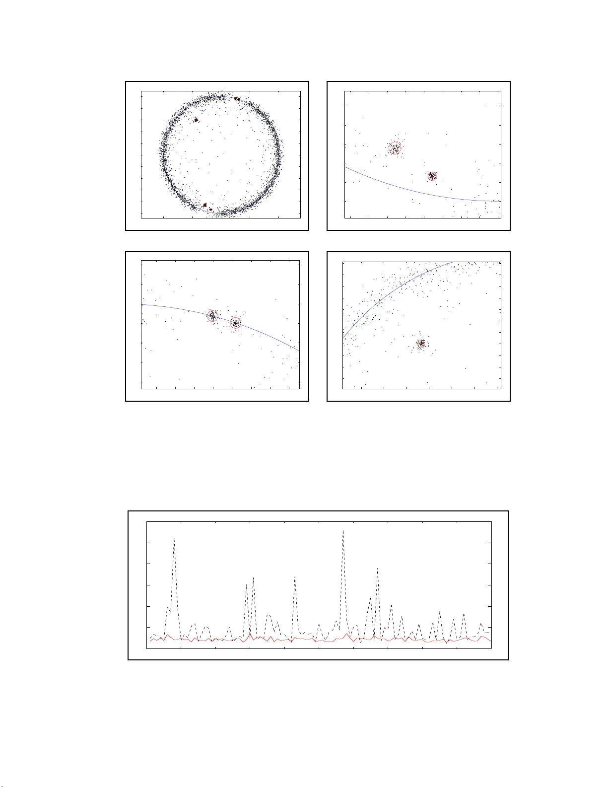
A new transform for solvin g the noisy complex exp on e n tials appro ximation p roblem P . Barone Istituto p er le A pplic a zioni del Calc olo ”M . Pic one”, C.N .R., Viale del Policlinic o 137, 00161 R ome, Italy e-mail: b ar one@iac.rm.cnr.it fax: 39-6-4404306 1 Abstract The problem of estima t ing a compl ex measure made up b y a linear combination of Dirac distr ibutio ns cen tered on p oints of the com plex plane from a finit e num- b er of its complex momen ts affected b y additi v e i.i.d. Gaussian noise i s considered . A random m easure is defined whose exp ectat ion appr o xi mates the unknown mea- sure u nd er suitable condit i ons. An estim a tor of t he ap pr o xi mati ng mea sure i s t hen prop o sed as w ell a s a new discr ete tr ansfor m of the noi sy mo men ts t ha t all o ws to compute a n estima t e of the unkn own measure. A small si m ula tion study is also p erfo r med to ex p erim en tal ly c heck the go o dness of the a pproximation s. Key wor ds and phr ases: Compl ex mom en ts; Pade’ appro xim an ts; logar ithmi c p o- ten ti als; ra ndom det ermina n ts; ra ndom p olynom ials; p encils of m atri ces 2 In tro duction Let u s consider the comp l ex measure defined o n a compact set D ⊂ I C by S ( z ) = p X j =1 c j δ ( z − ξ j ) , ξ j ∈ in t( D ) , c j ∈ I C and let b e s k = Z D z k S ( z ) dz = Z Z D ( x + iy ) k S ( x + iy ) dxdy , k = 0 , 1 , 2 , . . . the complex m o men ts. It turns out th a t s k = p X j =1 c j ξ k j . (1) Let u s assume to know an even n umber n ≥ 2 p of no i sy co mplex mo m en ts a k = s k + ν k , k = 0 , 1 , 2 , . . . , n − 1 where ν k is a complex Gaussian, zero m ea n, white noise, with fini te kno wn v ari- ance σ 2 . In the fo llowing a ll r andom qua n tit ies are deno ted by b old characters. W e w ant to esti mate S ( z ) fro m { a k } k =0 ,...,n − 1 . F rom eq uatio n (1) this i s equiv alent to estima t e p, c j , ξ j , j = 1 , . . . , p , which i s t he well known difficult problem of com plex exp onentials approximati on. The pro blem is cen tra l in ma n y di sciplin es and app ear s in t he lit eratur e in differen t forms and con text s (see e.g. [6,12,22,24,28]). The assumptio ns ab o ut the noise v a ri- ance (constant and k no wn) are made her e to si mplif y the a nalysi s. How ever in ma ny applica tions the noi se is an instrum en tal one whic h is w ell represen ted by a whit e noise, zero mean, G a ussian pro cess who se v ariance is known or easy t o estima te. A 3 t ypi ca l exampl e i s provided b y NMR sp ectroscopy (see e.g. [8]). In the noi sel ess case the probl em beco mes the co m plex exp onential in terp o lati on problem [14]. Co n d i tions for existence and unicity of the so l utio n are ([14, Th.7 .2c]) : detU 0 ( s ) 6 = 0 , detU 1 ( s ) 6 = 0 where U ( s 0 , . . . , s 2 p − 2 ) =                        s 0 s 1 . . . s p − 1 s 1 s 2 . . . s p . . . . . . s p − 1 s p . . . s 2 p − 2                        and U 0 ( s ) = U ( s 0 , . . . , s 2 p − 2 ) , U 1 ( s ) = U ( s 1 , . . . , s 2 p − 1 ) . In fa ct exactly n = 2 p noisel ess moments are sufficient t o full y retri ev e S ( z ) , wher e p = m ax n ∈ I N { n | det ( U ( s 0 , . . . , s n − 2 )) 6 = 0 } . Moreov er ( ξ j , j = 1 , . . . , p ) are the general ized eigen v alues of the p encil P = [ U 1 ( s ) , U 0 ( s )] i. e. t hey are the r o ots o f the p o lynomi al in the v ar iable z det [ U 1 ( s ) − z U 0 ( s )] and c j are relat ed to t he gener alized eigen vector u j of P b y c j = u T j [ s 0 , . . . , s p − 1 ] T . In fact fro m equat ion ( 1) we ha ve c = V − 1 [ s 0 , . . . , s p − 1 ] T where V = V ander ( ξ 1 , . . . , ξ p ) 4 is the squa re V andermond e ma trix b a sed on ( ξ 1 , . . . , ξ p ). But it easy to sho w ( see e.g. [2]) that U 0 ( s ) = V C V T , U 1 ( s ) = V C Z V T where C = diag { c 1 , . . . , c p } a nd Z = diag { ξ 1 , . . . , ξ p } . Therefor e u k = V − T e k is the right gen er alized ei gen vector of P corresp o nding to ξ k , where e k is the k − th col umn of the identit y ma trix I p of order p . Viceversa when s k = 0 , ∀ k it was prov ed in [1 5] t hat det [ U ( a 0 , . . . , a n − 2 )] = det [ U 0 ( a )] 6 = 0 ∀ n a. s. and det [ U ( a 1 , . . . , a n − 1 )] = det [ U 1 ( a )] 6 = 0 ∀ n a.s. . Moreov er a sso ciated to t he r andom p o lynom ial det [ U 1 ( a ) − z U 0 ( a )] (2) a conden sed densit y h n ( z ) ca n b e considered whi c h is the exp ect ed v a lue o f t he (rando m) norm alized counting mea sure on the zero s of this p o lynomi al i. e. h n ( z ) = 2 n E    n/ 2 X j =1 δ ( z − ξ j )    . It was prov ed in [ 1] t h a t if z = r e iθ , the margi nal condensed densit y h ( r ) n ( r ) w.r. to r of the gener alized eigenv a lues is a sympto t icall y i n n a Dir a c δ suppo rted o n the unit circle ∀ σ 2 . Moreov er for finite n t he t he marg i nal condensed densi t y w.r. to θ i s unifor m ly distribut ed on [ − π , π ]. Starti ng from the general ized eigenv al ues ξ j and 5 general ized eig en vectors u j of the p enci l P = [ U ( a 1 , . . . , a n − 1 ) , U ( a 0 , . . . , a n − 2 )] w e then define a fam ily o f r andom mea sures S n ( z ) = n/ 2 X j =1 c j δ ( z − ξ j ) where c j = u T j [ a 0 , . . . , a n/ 2 − 1 ] T and w e giv e co nditi o ns under whic h E [ S n ( z )] approx- imat es S ( z ) . Mo reov er w e define a discrete tra nsf o rm ( P -T ransfo r m) on a l atti ce of p oints on D , whic h is an un biased and consist en t esti mato r of E [ S n ( z )] on the latti ce th us providing a com putati onal device to sol v e the or igin a l probl em. In [4] the same problem w as afforded. The joint distri b u t ion of the coeffi cients of the rand o m p oly nomia l ( 2) (when s k 6 = 0 , ∀ k ) w as approximated b y a multi- v ariate Gaussia n distri butio n and a theorem b y Ha mmersl ey [7] w as used to co m - pute the asso ciat ed co ndensed density of its ro o t s. An heuri stic algor ithm was then used to iden ti f y the ma in p ea ks of t he co nd en sed density a nd to g et estim ates of p, ξ j and c j , j = 1 , . . . , p based on them. In the present work the idea s pr esen ted in [4] ar e put o n a mor e rig o rous mathem a tical framework. A different approximatio n of the condensed density i s co nsidered and an auto m atic estimati on pro cedure is prop o sed. The pa p er is org anized as follows. In the first sect ion w e study the distributi on of t he general ized eigenv a lues of the random p encil P and we give an easi l y com putabl e approximate expression of the asso ciated condensed densi t y . In sectio n 2 we consider the i d entifiabil i ty probl em for S ( z ) given the data a . Co nditi o ns for identifiability are given and the approximati on prop erties of E [ S n ( z )] are pro ved. In sectio n 3 the 6 P -transfor m is defined and its statist ical p r op er t ies are st udied. In sect ion 4 the pro cedur e for esti mati n g the para meters p , { ξ j , c j , j = 1 , . . . , p } of the unkno wn measure fro m the P -tra nsform is descri b ed. Fin a lly in section 5 some exp er imental results on synthetic da t a ar e r ep orted. 1 Distribution of t he generalized eigenv alues of the p encil P W e start by ma king some tec hni cal assum ptions on t he noise mo del. When s k = 0 ∀ k , we noticed in t he intro duct i on that ξ j are, asym p t otica lly on n , uni form l y distri buted on the unit circle. Ther efore, when s k 6 = 0 is gi v en b y (1), w e can a ssume that n p = n / 2 − p among the ξ j , j = 1 , . . . , n/ 2 ar e rel ated to noise an d then t hey ca n b e mo del ed for larg e n by ˜ ξ j = e 2 π ij n p i.e. b y unifor m ly spa ced det ermini stic g enerali zed eigenv al ues. Therefor e the V andermonde matrix based on ˜ ξ j , j = 1 , . . . , n p is simply given b y V = √ n p · F ∈ I C n p × n p where F hk = 1 √ n p e 2 π ihk n p is the di screte F our ier transfo rm mat rix. Hence ˜ c = V − 1 [ ν 0 , . . . , ν n p − 1 ] T = 1 √ n p F H [ ν 0 , . . . , ν n p − 1 ] T and ˜ c has a compl ex multiv ari ate Gaussian distr ibutio n with E [ ˜ c j ] = 0 and E [ ˜ c j ˜ c h ] = σ 2 n p δ j h . Based on these o bserv ation s w e define a new noi se pro cess a s ˜ ν k =                  P n p j =1 ˜ c j ˜ ξ k j , k < n p ν k , k ≥ n p 7 and w e a ssum e t ha t ˜ c is indep enden t of ν k , k ≥ n p . But then E [ ˜ ν k ] = 0 and E [ ˜ ν k ˜ ν h ] =                                P 1 ,n p i,j ˜ ξ k i ˜ ξ h j E [ ˜ c i ˜ c j ] = σ 2 n p P n p r =1 e 2 π ir ( k − h ) n p = σ 2 δ hk , k , h < n p P n p j =1 E [ ˜ c j ν h ] ˜ ξ k j = 0 , h ≥ n p , k < n p E [ ν k ν h ] = σ 2 δ hk , h, k ≥ n p W e hav e t hen prov ed the fo llowing Lemma 1 The r andom ve cto rs ν k and ˜ ν k , k = 0 , . . . , n − 1 ar e e qual in distribu - tion. As a consequence i n the foll o wi ng w e wil l use ˜ ν k witho ut lo ss of generality . Remark 1 We notic e that when s k 6 = 0 , if the signal- to-noise r atio is define d as S N R = 1 σ min h =1 ,p | c h | we have E [ | ˜ c j | 2 ] = σ 2 n p = min h =1 ,p | c h | 2 n p S N R 2 . If S N R ≫ r 1 n p then E [ | ˜ c j | 2 ] ≪ | c k | 2 , ∀ j, k . A basic resul t w hic h wil l b e used extensiv ely in t h e fo l lowing is g iv en by Lemma 2 L et T = ( T (1) , T (2) ) b e the tr ansformation th a t maps e very r e alizat i o n a (ø) of a to ( ξ ( ø) , c (ø)) given by a k (ø) = P n/ 2 j =1 c j (ø) ξ j (ø) k , k = 0 , . . . , n − 1 , wher e ø ∈ Ω and Ω is the sp ac e of events. Then T is a.s. one-t o -one. Mor e over, for σ → 0 8 and for j = 1 , . . . , n/ 2 E [ ξ j ] =                  ξ j + o ( σ ) j = 1 , . . . , p ˜ ξ j − p + o ( σ ) , j = p + 1 , . . . , n/ 2 E [ c j ] =                  c j + o ( σ ) , j = 1 , . . . , p o ( σ ) , j = p + 1 , . . . , n/ 2 pro o f F rom [15] we know that a.s. det [ U h ( ν ) ] 6 = 0 , h = 0 , 1. Moreov er, wi th probabi lity 1, ther e is no functi onal dep endence b etw een ν and s . Therefore a.s. det [ U h ( a )] 6 = 0 , h = 0 , 1. But then a.s. the compl ex exp o nen ti a l in ter p ol a tion pr oblem for a has an unique soluti on ∀ ø hence T is a.s. one-to -one. The seco nd part of the t hesis is based o n a T a yl or expansio n of T ar ound a suitabl e po in t x 0 . A natura l candi date for x 0 w oul d b e s . Ho wev er we noti ce tha t T (1) ( s ) is not defined if n > 2 p , a nd, as a consequence, al so T (2) ( s ) is not d efi ned in this case. T herefor e, b y using Lem m a 1, wit h o ut lo ss of g en er ality , w e assume tha t the noise is represen ted b y ˜ ν k i.e. a k =                  P p j =1 c j ξ k j + P n/ 2 j = p +1 ˜ c j − p ˜ ξ k j − p , k = 0 , . . . , n p − 1 P p j =1 c j ξ k j + ν k , k = n p , . . . , n − 1 where n p = n / 2 − p. W e then define a new sequence ˜ s k b y ˜ s k = p X j =1 c j ξ k j + σ α n/ 2 X j = p +1 ˜ ξ k j − p , α ≥ 2 , k = 0 , . . . , n − 1 9 and we consider the pr o cess a k as a p erturba tion of ˜ s k . Ther efore w e choo se x 0 = ˜ s and notice tha t T (1) (˜ s ) j =                  ξ j j = 1 , . . . , p ˜ ξ j − p , j = p + 1 , . . . , n/ 2 T (2) (˜ s ) j =                  c j j = 1 , . . . , p σ α , j = p + 1 , . . . , n/ 2 W e now prov e that eac h comp onen t of T (1) ( a ) is an an a lyti c funct ion of a when a b elong to small neig h b o r o f ˜ s . The pro of fol lows closel y [27][Th. 6.9. 8 ]. F or ea c h fixed ø, the p ol ynomi al φ ( z , a ) = det [ U 1 ( a ) − z U 0 ( a )] is a n anal ytic f unction of z and a . Let ˆ ξ b e a zero of φ ( z , ˜ s ) a nd K = { ζ || ζ − ˆ ξ | = r } , r > 0 b e a circle aro und ˆ ξ not containing any other gen er alized eigenv a l ue of the penci l ˜ P = [ U ( ˜ s 1 , . . . , ˜ s n − 1 ) , U ( ˜ s 0 , . . . , ˜ s n − 2 )] . W e wan t to show that K do es not pass through an y zer o of φ ( z , a ). In fa ct b y the definitio n of K it fol lows tha t inf ζ ∈ K | φ ( ζ , ˜ s ) | > 0 . But φ ( z , a ) dep ends co n tinuously on a , hence ther e exi st s B = { x ∈ I C n || x − ˜ s | < ρ } , ρ > 0 such tha t inf ζ ∈ K | φ ( ζ , a ) | > 0 , ∀ a ∈ B . 10 By t he princi ple of argument, the num b er of zero s of φ ( z , a ) wit hin K is given b y N ( a ) = 1 2 π i I K φ ′ ( z , a ) φ ( z , a ) dz , φ ′ = ∂ φ ∂ z which is co n tinuous in B ; hence 1 = N (˜ s ) = N ( a ) , a ∈ B . Moreov er the simple zer o ξ (ø) o f φ ( z , a ) i nsi de K admits t he repr esentation (see e.g . [21]) ξ (ø) = 1 2 π i I K z φ ′ ( z , a ) φ ( z , a ) dz . F or a ∈ B t he i n tegr and is an anal ytic funct ion of a a nd therefore a lso ξ (ø) is an analyt ic functio n o f a when a ∈ B . W e no w consider T (2) ( a ). W e notice that each comp o nen t can b e obtained as a rati onal fun ct ion of t he com p onents of T (1) ( a ) b y t he fo rmula c j = e T j V − H a , j = 1 , . . . , n/ 2 where V is t he V anderm o nde m atri x based on T (1) ( a ). Th er efore al so c j is a n anal ytic f unction of a when a ∈ B . As T ( h ) = T ( h ) R + iT ( h ) I is analy t ic for a ∈ B , T ( h ) R and T ( h ) I are real a nalyt ic functi o ns of a R , a I where a = a R + ia I , (e.g. [ 13][pg .99] ) . T herefore they admit a T aylor series expansion aro u nd ˜ s when a ∈ B : T ( h ) Rk ( a ) = T ( h ) Rk (˜ s ) + n − 1 X i =0 ∂ T ( h ) Rk ( a ) ∂ a Ri | a =˜ s [ a Ri − ˜ s Ri ] + n − 1 X i =0 ∂ T ( h ) Rk ( a ) ∂ a I i | a =˜ s [ a I i − ˜ s I i ] + 1 2 n − 1 X i =0 n − 1 X j =0 ∂ 2 T ( h ) Rk ( a ) ∂ a Ri ∂ a Rj | a =˜ s [ a Ri − ˜ s Ri ][ a Rj − ˜ s Rj ] + 11 1 2 n − 1 X i =0 n − 1 X j =0 ∂ 2 T ( h ) Rk ( a ) ∂ a I i ∂ a I j | a =˜ s [ a I i − ˜ s I i ][ a I j − ˜ s I j ] + n − 1 X i =0 n − 1 X j =0 ∂ 2 T ( h ) Rk ( a ) ∂ a Ri ∂ a I j | a =˜ s [ a Ri − ˜ s Ri ][ a I j − ˜ s I j ] + ... and analo gously fo r T ( h ) I k ( a ). T aki ng ex p ectat ions we get E [( a Ri − ˜ s Ri )] = [ s Ri − ˜ s Ri ] = σ α · C i , C i = n/ 2 X j = p +1 ˜ ξ i j − p E [( a Ri − ˜ s Ri )( a Rj − ˜ s Rj )] = E [( a Ri − s Ri + σ α C i )( a Rj − s Rj + σ α C j )] = σ 2 2 δ ij + σ 2 α C i C j and anal ogousl y fo r th e oth er ter ms. Rememberi ng the indep endence of t he real and imag inary part s of a k , w e fina l ly g et E [ T ( h ) k ( a )] = T ( h ) k (˜ s ) + o ( σ ) . ✷ W e start now the study of the distributi on in I C of t he generali zed eigen v alues of P by making some qua lita tive st atements a lready present in the li terat ure. F or eac h reali zatio n ø, let { c j (ø) , ξ j (ø) } , j = 1 , . . . , n/ 2 b e the solut ion of t he com p l ex exp onential interp ola tion probl em for the dat a a k (ø) , k = 0 , . . . , n − 1 . It is well known that w e can t hen define the Pade’ appr o xi mant [ n/ 2 − 1 , n/ 2]( z , ø) = z n/ 2 X j =1 c j (ø) z − ξ j (ø) = Q n/ 2 − 1 ( z − 1 ) /P n/ 2 ( z − 1 ) to the Z − transfo rm of { a k (ø) } given b y f ( z , ø ) = ∞ X k =0 a k (ø) z − k = f s ( z ) + f ν ( z , ø) 12 where f s ( z ) = ∞ X k =0 s k z − k = p X j =1 c j ∞ X k =0 ( ξ j /z ) k = z p X j =1 c j z − ξ j , | z | > 1 and, b ecause of Lemm a 1 , f ν ( z , ø) ≈ z n p X j =1 ˜ c j (ø) z − ˜ ξ j f ( z , ø ) is then defined out side the unit circle an d ca n b e ext ended to D by a nalyt i c con ti n uati on. W e get th en f ( z , ø ) ≈ z ˜ q n/ 2 − 1 ( z ) / ˜ p n/ 2 ( z ) = z Q n/ 2 − 1 j =1 ( z − δ j (ø)) Q p j =1 ( z − ξ j ) Q n p j =1 ( z − ˜ ξ j ) and g ( z , ø) = log ( z − 1 f ( z , ø )) = n/ 2 − 1 X j =1 log( z − δ j (ø)) − p X j =1 log( z − ξ j ) − n p X j =1 log( z − ˜ ξ j ) . W e wan t to study the lo cati on in I C of ξ j (ø). T o this aim, fo llowing [19], w e remember that p n ( z ) = z n P n ( z − 1 ) sa tisfy the following o r thogo nality rela tion Z Γ z − 1 f ( z , ø ) p n ( z ) z k dz = 0 , k = 0 , . . . , n − 1 where Γ is a union of cl osed curv es enclosing the p oles of f ( z , ø) i. e. t he num b ers ξ j , j = 1 . . . , p and ˜ ξ j , j = 1 , . . . , n p . By usin g t he Szego i n tegr al repr esen tat i on of suc h p olynom i als a nd a sa ddle p oint argument, it tur ns out that the P ade’ p o les ξ j (ø) , j = 1 , . . . , n/ 2 , asympt o tical ly on n , satisfy t he following system of algebr aic equati o ns 2 1 ,n/ 2 X j 6 = k 1 ( ξ k (ø) − ξ j (ø)) + g ′ ( ξ k (ø)) = 0 k = 1 , . . . , n/ 2 or 13 2 1 ,n/ 2 X j 6 = k 1 ( ξ k (ø) − ξ j (ø)) + n/ 2 − 1 X j =1 1 ( ξ k (ø) − δ j (ø)) + − p X j =1 1 ( ξ k (ø) − ξ j ) − n p X j =1 1 ( ξ k (ø) − ˜ ξ j ) = 0 , k = 1 , . . . , n/ 2 These equations can b e in terpr eted as conditions o f electrost a tic equil i brium of a set o f c har ges in the pr esence of an elect r ic ext er nal field corresp o nding to g ′ ( z , ø) . Therefor e t he Pade’ p o les ξ k (ø) a re att racted b y ξ j , j = 1 , . . . , p and ˜ ξ j , j = 1 , . . . n p and they ar e r ep elled by eac h o ther a nd b y t he zer os δ j (ø) of ˜ q n/ 2 − 1 ( z ). H ow ev er ˜ q n/ 2 − 1 ( z ) = p X j =1 c j 1 ,p Y k 6 = j ( z − ξ k ) n p Y k =1 ( z − ˜ ξ k ) (3) + n p X j =1 ˜ c j (ø) p Y k =1 ( z − ξ k ) 1 ,n p Y k 6 = j ( z − ˜ ξ k ) . (4) As ∀ ø , | ˜ c j (ø) | 2 ≪ min h | c h | 2 if the SNR is suffi cien tl y hi gh (see Rema rk after Lemm a 1), w e ca n ap pr o xi mate ˜ q n/ 2 − 1 ( z ) b y n p Y k =1 ( z − ˜ ξ k ) p X j =1 c j 1 ,p Y k 6 = j ( z − ξ k ) hence n p zeros are close to ˜ ξ k , a nd the other p − 1 are close to th e zeros o f the p oly nomia l q p − 1 ( z ) = p X j =1 c j 1 ,p Y k 6 = j ( z − ξ k ) which is t he n umer ator o f z − 1 f s ( z ). W e no tice that if | c h | ≪ | c k | , ∀ k 6 = h then q p − 1 ( z ) ≈ 1 ,p X j 6 = h c j 1 ,p Y k 6 = j ( z − ξ k ) = ( z − ξ h ) p X j =1 c j 1 ,p Y k 6 = j,h ( z − ξ k ) Hence, b ecause of the contin uous dep endence of t he ro o t s from the co effi ci en t of a pol ynomi al, q p − 1 ( z ) has a zero as close to ξ h as | c h | is smal l w ith r esp ect to | c k | , k 6 = h . T h er efore t he Pade’ p o l es ξ k (ø) 14 • are a ttra ct ed b y ξ j , j = 1 , . . . , p • are a ttra ct ed b y ˜ ξ j , j = 1 , . . . n p • are r ep elled fr om ξ j (ø) , j 6 = k • are r ep elled fr om ˜ ξ j , j = 1 , . . . n p • are r ep elled from ot h er p − 1 p oi n ts in the complex plane which are as close to ξ j as | c j | is sma l l wi th resp ect to | c h | , h 6 = j . Summing up a ξ k with a large | c k | wi ll attr act a P ade’ p ole w ithout b ei ng dist urb ed b y th e rep ul sion exert ed b y the zeros of ˜ q n/ 2 − 1 ( z ). Mo reov er clo se to such a p oi n t a gap of Pade’ p o les can b e exp ect ed b ecause of the r epu l sion exerted by Pade’ p o les to each other . A ξ k with a smal l | c k | wi ll sti ll a ttra ct a Pade’ p o le bu t not so clo se b ecause o f the repulsio n exerted by a close zero. The Pade’ p oles not rela ted to the signal ar e exp ect ed to b e attra cted by ˜ ξ k which at the sa me tim e w ill r ep el th em . Moreov er they a re r ep ell ed by ξ k hence they are likely to b e l o cat ed in b etw een ˜ ξ k and far f rom ξ k . A pi cture of t his b ehavior is given in fig.1 . W e notice th a t the quali t ative results discussed ab o ve ar e co nsistent with those obtained in [3] under a more string en t hyp o thesis ab o ut the noise. W e now wish to d efin e a ma themat ical t o ol to quantify th ese qu a lita tive sta t ements. T o this aim we remember that ξ k , k = 1 , . . . , n/ 2 are the genera lized eig env a lues of the p encil P a nd t h er efore they sat isfy t he equation P n/ 2 ( z − 1 ) = det [ U 1 ( a ) − z U 0 ( a )] = 0 . 15 Then a condensed densit y h n ( z ) can b e consider ed whi c h i s the exp ected v alue of the (rando m) no rmal ized coun ti ng mea sure on the zero s of this p olynom ial i. e. h n ( z ) = 2 n E    n/ 2 X j =1 δ ( z − ξ j )    . The f ollowing theor em hol d s who se pro of is t he sam e of that o f T heorem 1 in [1]: Theorem 1 The c onden s e d density of the zer os of th e r andom p olynomial Q ( z ) = P n/ 2 ( z − 1 ) is given by h n ( z ) = 1 4 π ∆ u n ( z ) (5) wher e ∆ denotes the L aplacian op er ator wi t h r esp e ct to x, y if z = x + iy and u n ( z ) = 2 n E n log ( | Q ( z ) | 2 ) o (6) The conden sed densit y provides the required quantitative informat ion ab o u t the distri bution of t he Pade’ p o les in the complex plane. If the SNR is sufficien tl y high, after the quali tati v e statements ma de ab ov e ab out the l o cat ion of the P ade’ p oles, a p eak of h n ( z ) can b e exp ected i n a neighbor ho o d of eac h of the comp l ex exp o nen tia ls ξ k , k = 1 , . . . , p a nd the volume under the peak give s the pr o babil i t y of finding a P ade’ p ol e in that nei gh b orho o d. This i s co n fi r med b y t he fo llowing Theorem 2 If σ > 0 , the c onden se d de nsity h n ( z , σ ) is a c on t i n uous function of z given by h n ( z , σ ) = 2 n ( π σ 2 ) n n/ 2 X j =1 Z I C n/ 2 − 1 Z I C n/ 2 J ∗ C ( ζ ∗ j , z , γ ) e − 1 σ 2 P n − 1 k =0 | P 1 ,n/ 2 h 6 = j γ h ζ k h + γ j z k − s k | 2 dζ ∗ j dγ (7) 16 wher e ζ ∗ j = { ζ h , h 6 = j } and J ∗ C ( ζ ∗ j , z , γ ) =                  γ if n = 2 ( − 1) n/ 2 Q 1 ,n/ 2 j =1 γ j Q r 2 p . W e cannot use the same arg u m en t used fo r the ca se n = 2 p b ecause ζ j ( s ) i s no t defined for j = p + 1 , . . . , n/ 2 ( see Lemm a 2) . Ho wev er by Lemm a 1 without loss of general i t y , w e can assum e that the noise is represented b y ˜ ν k i.e. a k =                  P p j =1 c j ξ k j + P n/ 2 j = p +1 ˜ c j − p ˜ ξ k j − p , k = 0 , . . . , n p − 1 P p j =1 c j ξ k j + ν k , k = n p , . . . , n − 1 where n p = n / 2 − p. W e t hen define a new pr o cess ˜ a k b y ˜ a k = p X j =1 c j ξ k j + η k , k = 0 , . . . , n − 1 where η k = n/ 2 X j = p +1 ˜ c j − p ˜ ξ k j − p , and we consider the pro cess a k as a p erturba tion of t he pr o cess ˜ a k . Let us consider the p encils P = [ U ( a 1 , . . . , a n − 1 ) , U ( a 0 , . . . , a n − 2 )] and ˜ P = [ U ( ˜ a 1 , . . . , ˜ a n − 1 ) , U ( ˜ a 0 , . . . , ˜ a n − 2 )] . W e can w rite P = ˜ P + σ E where E = 1 σ [ U (0 , . . . , 0 , ν n p +1 − η n p +1 , . . . , ν n − 1 − η n − 1 ) , U (0 , . . . , 0 , ν n p − η n p , . . . , ν n − 2 − η n − 2 )] = [ E 1 , E 0 ] . 19 F r om [16], in the lim i t for σ → 0, a gener alized eigen v alue ξ j of P can b e expressed as a functio n of a general ized ei gen v alue ˆ ξ j of ˜ P and cor resp ondi ng l eft and ri g h t general ized eig en vectors v j , u j b y ξ j = ˆ ξ j + σ v H j ( E 1 − ˆ ξ j E 0 ) u j v H j U 0 u j + O ( σ 2 ) = ˆ ξ j + σ e T j V − 1 ( E 1 − ˆ ξ j E 0 )) V − T e j ˆ c j + O ( σ 2 ) where U 0 = U ( ˜ a 1 , . . . , ˜ a n − 1 ) a nd, b y co nstructi on, ˆ ξ j =                  ξ j j = 1 , . . . , p ˜ ξ j − p , j = p + 1 , . . . , n/ 2 ˆ c j =                  c j j = 1 , . . . , p ˜ c j − p , j = p + 1 , . . . , n/ 2 V = V ander ( ˆ ξ 1 , . . . , ˆ ξ n/ 2 ) , C = diag ( ˆ c 1 , . . . , ˆ c n/ 2 ) and v j = u j = V − H e j . W e notice that we can wr ite e T j V − 1 ( E 1 − ˆ ξ j E 0 ) V − T e j = n/ 2+ p X h =1 γ j h Y n p + h where γ j h are constants and Y h ( are i.i. d. zero mean, com p l ex Gaussia n v ar i ables with unit v ar i ance identified w ith 1 √ 2 σ [ ν h − η h ] , h = n p , . . . , n − 1. W e ha v e 20 h n ( z , σ ) = 2 n E    n/ 2 X j =1 δ ( z − ξ j )    = 2 n E   p X j =1 δ ( z − ξ j )   + 2 n E    n/ 2 X j = p +1 δ ( z − ξ j )    = h (1) n ( z , σ ) + h (2) n ( z , σ ) By t he sam e arg umen t used for t he ca se n = 2 p i t fol lows that h (1) n ( z , σ ) con v erg es w eakl y to 2 n P p j =1 δ ( z − ξ j ) when σ → 0. W e then consi der h (2) n ( z , σ ). W e hav e h (2) n ( z , σ ) = 2 n E    n/ 2 X j = p +1 δ ( z − ξ j )    = 2 n E    n/ 2 X j = p +1 δ    z − ˜ ξ j − p − σ P n/ 2+ p h =1 γ j h Y n p + h ˜ c j − p − O ( σ 2 )       . By iden ti fying √ n p σ ˜ c j − p , j = p + 1 , . . . , n/ 2 wi t h Y h , h = 1 , . . . , n p , whic h are i.i. d. zero mean, co mplex G a ussian v ariab l es wit h uni t v ar iance, w e get h (2) n ( z , σ ) = n/ 2 X j = p +1 Z I C n δ    z − ˜ ξ j − p − √ n p y j − p n/ 2+ p X h =1 γ j h y n p + h − O ( σ 2 )    e − 1 σ 2 P n k =1 | y k | 2 π n dy = n/ 2 X j = p +1 Z I C n − 1    Z I C δ    z − ˜ ξ j − p − √ n p y j − p n/ 2+ p X h =1 γ j h y n p + h − O ( σ 2 )    e −| y j − p | 2 π dy j − p    · e − P n k =1 ,k 6 = j − p | y k | 2 π n − 1 dy ′ , { y ′ } = { y } \ { y j − p } (10) b y maki ng the c ha nge o f v ar iable w = ˜ ξ j − p + √ n p y j − p n/ 2+ p X h =1 γ j h y n p + h w e get Z I C δ    z − ˜ ξ j − p − √ n p y j − p n/ 2+ p X h =1 γ j h y n p + h − O ( σ 2 )    e −| y j − p | 2 π dy j − p 21 = − 1 π Z I C δ  z − w − O ( σ 2 )  √ n p P n/ 2+ p h =1 γ j h y n p + h ( w − ˜ ξ j − p ) 2 e −      √ n p P n/ 2+ p h =1 γ j h y n p + h w − ˜ ξ j − p      2 dw = − 1 π √ n p P n/ 2+ p h =1 γ j h y n p + h ( z − O ( σ 2 ) − ˜ ξ j − p ) 2 e −      √ n p P n/ 2+ p h =1 γ j h y n p + h z − O ( σ 2 ) − ˜ ξ j − p      2 . Inserting this ex pression i n (10) we get h (2) n ( z , σ ) = − n/ 2 X j = p +1 √ n p ( z − O ( σ 2 ) − ˜ ξ j − p ) 2 · n/ 2+ p X r =1 γ j r 1 π n Z I C n − 1 y n p + r e −      √ n p P n/ 2+ p h =1 γ j h y n p + h z − O ( σ 2 ) − ˜ ξ j − p      2 − P n k =1 ,k 6 = j − p | y k | 2 dy ′ and therefo r e lim σ → 0 h (2) n ( z , σ ) = − n/ 2 X j = p +1 √ n p ( z − ˜ ξ j − p ) 2 · n/ 2+ p X r =1 γ j r 1 π n Z I C n − 1 y n p + r e −      √ n p P n/ 2+ p h =1 γ j h y n p + h z − ˜ ξ j − p      2 − P n k =1 ,k 6 = j − p | y k | 2 dy ′ = 0 b ecause 1 π n − 1 Z I C n − 1 y n p + r e −      √ n p P n/ 2+ p h =1 γ j h y n p + h z − ˜ ξ j − p      2 − P n k =1 ,k 6 = j − p | y k | 2 dy ′ = 1 π n − 1 Z I C n − 1 y n p + r e − y ′ H Ay ′ dy ′ = 0 , for a suitable hermit ian m atri x A, ∀ r . ✷ Remark . When the SNR i s l arge t he exp onential part domi nates the integrand as the Jacobian do es not dep end on σ . Moreov er the exp o nen ti a l pa r t ha s relative maxim a close t o ξ j as ex p ected. In genera l the in teg ral (7) do es not admi t a clo sed form expressio n. How ever when n = 2, r ememberi ng that t he Jacobi an w ith resp ect 22 to the real a n d imagina ry part of a co mplex v ariabl e is J R = | J C | 2 , the integral (7) b ecomes h 2 ( z , σ ) = 1 ( π σ 2 ) 2 Z I C γ e − | γ − s 0 | 2 + | γ z − s 1 | 2 σ 2 dγ = 1 ( π σ 2 ) 2 Z I R 2 | γ | 2 e − | γ − s 0 | 2 + | γ z − s 1 | 2 σ 2 d ℜ γ d ℑ γ = σ 2 (1 + | z | 2 ) + | z s 1 + s 0 | 2 π σ 2 (1 + | z | 2 ) 3 e − | z s 0 − s 1 | 2 σ 2 (1+ | z | 2 ) . W e notice that lim σ → 0 h 2 ( z , σ ) = δ ( z − s 1 /s 0 ) = δ ( z − ξ 1 ). Moreo ver, when s 0 = s 1 = 0 w e hav e h 2 ( z , σ ) = 1 π (1+ | z | 2 ) 2 which is indep endent of σ 2 , confir ming the result obtai ned in [ 1] fo r the pure noi se case. The co ndensed densit y ha s a n imp ort a n t role in t he following. T herefor e w e lo ok for an easily comput able approximatio n. The following theo rem provides a ba sis for buildin g suc h a n approximati on : Theorem 3 L et b e F ( z , z ) = ( U 1 ( a ) − z U 0 ( a ))( U 1 ( a ) − z U 0 ( a )) then E [log( d et { F ( z , z ) } )] − lo g( det { E [ F ( z , z )] } ) = o ( σ ) for σ → 0 , indep en d e ntly of z. Mor e over E [ F ( z , z )] = ( U 1 ( s ) − z U 0 ( s ))( U 1 ( s ) − z U 0 ( s )) + nσ 2 2 A ( z , z ) (11) 23 wher e A ( z , z ) =                        1 + | z | 2 − z 0 . . . 0 − z 1 + | z | 2 − z 0 . . . . . . . . 0 . . . 0 − z 1 + | z | 2                        . pro o f let us denote b y λ j the eigen v alues of F ( z , z ) and b y µ j those of E [ F ( z , z )] , dropping for simpl icity the dep endence on z , z . No te that µ j 6 = E [ λ j ], see e.g. [5, Theo rem 8.5] . W e ha ve E [log ( det { F ( z , z ) } ) ] = X j E [log( λ j )] and log( det { E [ F ( z , z )] } ) = X j log( µ j ) hence it is suffi cien t to study the di fference E [log ( λ j )] − l og( µ j ) . W e then d eno te by f the vector obta i ned by stacking t he real and im agina ry part s of the elem en ts ( F hk , h, k = 1 , . . . , n/ 2) o f F and consider the funct ion g ( f ) = log( λ j ) and its T aylor expansi o n a round E [ f ]: 24 g ( f ) = g ( E [ f ] ) + X h ∂ g ∂ f h    E [ f ] ( f h − E [ f h ]) + 1 2 X hk ∂ 2 g ∂ f h ∂ f k    E [ f ] ( f h − E [ f h ])( f k − E [ f k ]) + . . . which can b e rew ritt en as log ( λ j ) − log( µ j ) = X h β h ( f h − E [ f h ]) + 1 2 X hk γ hk ( f h − E [ f h ])( f k − E [ f k ]) + . . . and, tak i ng exp ectatio ns, E [log( λ j )] − l og ( µ j ) = 1 2 X hk γ hk E [( f h − E [ f h ])( f k − E [ f k ])] + . . . But F ( z , z ) = ( U 1 ( s ) − z U 0 ( s )( U 1 ( s ) − z U 0 ( s )) + ( U 1 ( ν ) − z U 0 ( ν ) ) ( U 1 ( ν ) − z U 0 ( ν ) ) − ( U 1 ( s ) − z U 0 ( s )( U 1 ( ν ) − z U 0 ( ν ) ) − ( U 1 ( ν ) − z U 0 ( ν ) ) ( U 1 ( s ) − z U 0 ( s )) and E [ F ( z , z )] = ( U 1 ( s ) − z U 0 ( s )( U 1 ( s ) − z U 0 ( s )) + E [ ( U 1 ( ν ) − z U 0 ( ν ) ) ( U 1 ( ν ) − z U 0 ( ν ) )] = ( U 1 ( s ) − z U 0 ( s )( U 1 ( s ) − z U 0 ( s )) + nσ 2 2 A ( z , z ) b y a str a ightforw ar d com putat i on simil ar to tha t g iven in [1, Th.3] fo r t he pure noise case. Theref ore F ( z , z ) − E [ F ( z , z )] = ( U 1 ( ν ) − z U 0 ( ν ))( U 1 ( ν ) − z U 0 ( ν ) ) − ( U 1 ( s ) − z U 0 ( s )( U 1 ( ν ) − z U 0 ( ν )) − ( U 1 ( ν ) − z U 0 ( ν ))( U 1 ( s ) − z U 0 ( s )) − nσ 2 2 A ( z , z ) 25 hence E [( f h − E [ f h ])( f k − E [ f k ])] i s a linear combination of functi ons of z and z wit h co effici en ts equal to either σ 2 or σ 4 b ecause the o dd mom en ts of a Gaussian a re zero. By a simil ar ar gument all the dropp ed ter m s i n the T aylor expansion ab ov e will dep end o n even p ow ers of σ . Hence E [log( λ j )] − l og ( µ j ) = o ( σ ) indep endently of z , z . ✷ By noticing that | Q ( z ) | 2 = d et { F ( z , z ) } , an approximati on of the condensed density is t hen given b y ˜ h n ( z , σ ) = 1 2 π n ∆ X µ j ( z ) > 0 log( µ j ( z )) where µ j ( z ) are t he ei gen v alues o f E [ F ( z , z )] . Unfo rtunat ely ˜ h n ( z , σ ) is not a prob- abili t y density as it ca n even tuall y assume nega tive v al ues. How ever the following results hol d Theorem 4 The funct i o n ˜ h n ( z , σ ) is c ontinuous in σ and in z . In the limit c as e s σ = 0 and { c k = 0 , k = 1 , . . . , p } it is given r esp e ctively by ˜ h n ( z , 0) = 2 n p X j =1 δ ( z − ξ j ) and by ˜ h n ( z , σ ) = 1 4 π ∆ w n ( z ) wher e w n ( z ) = 1 n log n X j =0 | z | 2 j . Mor e over, in this se c ond c as e, lim n →∞ ˜ h n ( z , σ ) = δ ( | z | − 1) . pro o f 26 ˜ h n ( z , σ ) is con ti n uous i n σ and in z because of the con ti n uous dep endence o f t he eigenv al ues on the elements of the corresp onding matri x . When σ = 0, let V ∈ I C n/ 2 ,p b e the V anderm onde m atri x suc h that U 0 ( s ) = V C V T and U 1 ( s ) = V C Z V T . Let V = QR b e the QR decomp osit ion of V . Then E [ F ( z , z )] = Q RC ( Z − z I ) R T Q T QR ( Z − z I ) C R H Q H . But R =          ˜ R 0          , therefor e R T R = ˜ R T ˜ R ; mor eov er Q T Q = I , hence the eigen v alues of E [ F ( z , z ) ] a re the sam e of those o f t he matr ix RC ( Z − z I ) R T R ( Z − z I ) C R H =          ˜ RC ( Z − z I ) ˜ R T ˜ R ( Z − z I ) C ˜ R H 0 0 0          . The n o n-zero eigenv a lues of E [ F ( z , z )] a re then the sam e of those of the mat rix ˜ RC ( Z − z I ) ˜ R T ˜ R ( Z − z I ) C ˜ R H . W e then ha ve ˜ h n ( z , 0) = 1 2 π n ∆ X µ j ( z ) > 0 log( µ j ( z )) = 1 2 π n ∆ log   p Y j =1 | z − ξ j | 2 · | det ( ˜ R ) | 4 p Y j =1 c 2 j   = 2 4 π n p X j =1 ∆ log | z − ξ j | 2 = 2 n p X j =1 δ ( z − ξ j ) b ecause 1 4 π ∆ log( | z | 2 ) = δ ( z ) (see e.g. [ 25, pg.47 ]). When { c k = 0 , k = 1 , . . . , p } 27 ˜ h n ( z , σ ) = 1 2 π n ∆ log( d et { A ( z , z ) } ) = 1 2 π n ∆ log ( n X j =0 | z | 2 j ) . The last pa rt of t he thesis follows b y the same argument used in th e pro of of Theorem 3 i n [ 1] . ✷ Corollary 2 ˜ h n ( z , σ ) − h n ( z , σ ) c onver ges we akly to 0 when σ → 0 pro o f Let Φ( z ) b e a nonnegati v e test functi on supp orted o n I C . Denoti ng b y h ∗ n ( z ) = 2 n P p j =1 δ ( z − ξ j ), fro m Theo rems 2 and 4 we hav e ∀ ν > 0 , ∃ σ 1 and σ 2 > 0 suc h that        Z I C Φ( z ) ( h n ( z , σ ) − h ∗ n ( z )) dz        < ν 2 , ∀ σ < σ 1 and        Z I C Φ( z )  ˜ h n ( z , σ ) − h ∗ n ( z )  dz        < ν 2 , ∀ σ < σ 2 hence, if σ ν = m in { σ 1 , σ 2 } , w e hav e ∀ σ < σ ν        Z I C Φ( z )  h n ( z , σ ) − ˜ h n ( z , σ )  dz        ≤        Z I C Φ( z ) ( h n ( z , σ ) − h ∗ ( z )) dz        +        Z I C Φ( z )  ˜ h n ( z , σ ) − h ∗ ( z )  dz        ≤ ν . ✷ 2 Iden tifiabilit y of S ( z ) and approxim ation prop ert ies of E [ S n ( z )] W e wan t now to exploit t he i nform atio n ab out the l o cati o n in the com plex pl ane of the P ade’ p oles, provided b y the condensed density h n ( z ), to pro ve som e prop er ties relat ing S n ( z ) = P n/ 2 j =1 c j δ ( z − ξ j ) t o the tr ue m easure S ( z ). 28 Before affording the problem of esti mati ng S ( z ) from the data a we need to c heck that the data pro vi d e enou g h i nforma tion to solv e i t. Pr ecise conditions tha t must b e met to solve the problem are w ell kno wn in the noiseless case and are rep ort ed in t he intro ductio n. When noise is pr esent the i den tifia bility pro blem is an o p en one. Its so lv ability ca n dep end on the am oun t of ”a prio ri” i nform a tion av a ilabl e [6] and/or on the abil ity to devise sma rt algor ithms. In the foll o wi ng a definiti on of iden ti fiabil i t y is given and, based o n i t, some prop erties of S n ( z ) ar e pr ov ed. Definition 1 The m e a sur e S ( z ) is identifi able fr om the data a k , k = 0 , . . . , n − 1 if ∃ r k > 0 , k = 1 , . . . , p such that • h n ( z ) is unimo dal in N k = { z | | z − ξ k | ≤ r k } • T p k =1 N k = ∅ The idea is that S ( z ) can b e identified from the data a if the random general- ized eigenv a lues ha ve a co ndensed density with separat e p eaks centered on ξ j , j = 1 , . . . , p . As, b y Theo rem 2, h n ( z , σ ) con verges w eakl y to 2 n P p j =1 δ ( z − ξ j ) when σ → 0, i t must exi sts a σ ′ > 0 sm all enoug h t o m ake S ( z ) i den tifia ble ∀ σ < σ ′ . In order to a p p l y t he pro p osed metho d one shoul d c hec k th a t the identifiabili t y conditi ons are verified. As h n ( z , σ ) depends on the unkno wn q uan ti ties p, c j , ξ j this is of course imp o ssi ble. Ho wev er i n most real problems w e ha ve some prior infor mati on ab out the unk no wn mea sure S ( z ) that we can explo it to get reaso nable i nterv al estima t es for p , c j , ξ j . Moreo v er i n m an y instances eit h er n or σ o r b oth can b e freely chosen. By Theorem 3, equatio n 11, n should not b e a s la r ge as p ossible to get the b est estimates o f S ( z ). In fact t o o many dat a will conv ey to o m uc h no ise 29 which could mask the signal s k . W e can ther efore pro p erly desi gn an exp erim en t by computi ng h n ( z , σ ) for many v alues of n an d σ a nd c ho ose n ott and σ ott (opti mal design) t h a t make iden ti fiable the m easures corr esp ondi ng to prior est i mates o f p, c j , ξ j . T o i den ti fy the u n k no wn mea sure S ( z ) we then hop efully need to mea sure n ott data a ffected b y an er ror with s.d. σ ott . Unfor tunatel y h n ( z ) do es not adm it a closed form expression and to com pute the exp ectat i on t hat app ea rs in its definitio n w e need to p er form a time consumi ng MonteCarlo exp eriment. This is wh y w e prop o sed an appr oximat i on ˜ h n ( z ) o f h n ( z ) whi ch ca n be quic kly comp ut ed b y solving hermit ian eigenv a lues pro blems. Let u s consider the functi on S n ( z ) = E [ S n ( z )] = n/ 2 X j =1 E [ c j δ ( z − ξ j ] where { c j , ξ j } , j = 1 , . . . , n/ 2 } are the solutio n of the co mplex exp onential in ter - p ola tion pro blem f or the da t a { a k , k = 0 , . . . , n − 1 } . The rela t ion betw een S n ( z ) and the un k no wn measur e S ( z ) i s given by the following Theorem 5 If S ( z ) is identifiab l e fr om a then Z N h S n ( z ) dz = c h + o ( σ ) and Z A S n ( z ) dz = o ( σ ) , ∀ A ⊂ D − [ j N j pro o f 30 F r om the i den tifia bility h yp othesis we kno w that Z N k h n ( z ) dz = 2 n n/ 2 X j =1 P rob [ ξ j ∈ N k ] > 0 , k = 1 , . . . , p. Therefor e there exist ξ j k suc h that P rob [ ξ j k ∈ N k ] > 0. Am ong the ξ j k let u s denote b y ξ ˆ k the o n e such t ha t P r ob [ ξ j k ∈ N k ] is maxi m um. F rom the identifiabili t y h yp o thesis th e ξ ˆ k are disti nct. Mor eo ver a ll the ξ j , j = 1 , . . . , n/ 2 can b e sorted in suc h a w ay th a t ξ j = ξ ˆ j , j = 1 , . . . , p and, b y Lemma 2, to ξ k it cor resp onds c k suc h tha t E [ c k ] =                  c k + o ( σ ) , k = 1 , . . . , p o ( σ ) , k = p + 1 , . . . , n/ 2 But then fo r k = 1 , . . . , p Z N k S n ( z ) dz = n/ 2 X j =1 Z N k E [ c j δ ( z − ξ j ] dz = = n/ 2 X j =1 Z N k    Z I C 2 γ δ ( z − ζ ) dµ γ ζ    dz = = n/ 2 X j =1 Z I C 2 γ    Z N k δ ( z − ζ ) dz    dµ γ ζ where µ γ ζ is t he joint distri bution o f c j and ξ j . W e hav e Z N k δ ( z − ζ ) dz =                  1 if ζ ∈ N k 0 otherw ise hence, Z N k S n ( z ) dz = n/ 2 X j =1 E [ c j δ j k ] = E [ c k ] = c k + o ( σ ) . By a simila r argum en t t he second part of the th esi s fo llows. ✷ 31 3 The P -transform In order to so lve the o r igina l moment problem we need t o co mpute S n ( z , σ 2 ) = n/ 2 X j =1 E [ c j δ ( z − ξ j ] . In order to esti mate the exp ect ed v alue we build indep endent replicati ons o f the data (pseudosam ples) by defini ng a ( r ) k = a k + ν ( r ) k , k = 0 , . . . , n − 1; r = 1 , . . . , R where { ν ( r ) k } ar e i.i.d. zero mea n co mplex Gaussia n v ariabl es wit h v ariance σ ′ 2 in- dep endent of a h , ∀ h . Therefore E [ a ( r ) k ] = s k , E [ ( a ( r ) k − s k )( a ( s ) h − s h )] = ˜ σ 2 δ hk δ rs where ˜ σ 2 = σ 2 + σ ′ 2 . F o r r = 1 , . . . , R , we define t he stati stics ˆ S n,r ( z , ˜ σ 2 ) = n/ 2 X j =1 c ( r ) j δ ( z − ξ ( r ) j ) where c ( r ) j , ξ ( r ) j are t he sol ution of the com plex exp onen tia ls in terp olat ion problem for the data a ( r ) k , k = 0 , . . . , n − 1 . A s, by Lem ma 2, the tr a nsform a tion T : { a ( r ) k , k = 0 , . . . , n − 1 } → { [ c ( r ) j , ξ ( r ) j ] , j = 1 , . . . , n/ 2 } is one-to -one, ˆ S n,r ( z , ˜ σ 2 ) are i. i.d. wi t h mean S n ( z , ˜ σ 2 ) and fini te v aria nce ζ ( z , ˜ σ 2 ) b ecause { ν ( r ) k } are i. i.d. . Therefo r e the st atist i c ˆ S n,R ( z , ˜ σ 2 ) = 1 R R X r =1 ˆ S n,r ( z , ˜ σ 2 ) has mean S n ( z , ˜ σ 2 ) = E [ ˆ S n,r ( z , ˜ σ 2 )] and v arian ce 1 R ζ ( z , ˜ σ 2 ) . 32 Let u s consider the stat istic ˆ S n ( z , σ 2 ) = n/ 2 X j =1 c j δ ( z − ξ j ) where c j , ξ j are the solut i on of t he com plex exp onen ti als i n terp olat ion pr oblem for the data a k , k = 0 , . . . , n − 1 a nd t he condit ioned st atist ic ˆ S c n,R ( z , ˜ σ 2 ) = ˆ S n,R ( z , ˜ σ 2 ) | a which are b ot h com putabl e from the o bserv ed data a . W e ha v e Lemma 3 F or n and σ > 0 fixe d and ∀ z and ˜ σ , E [ ˆ S c n,R ( z , ˜ σ 2 )] = S n ( z , ˜ σ 2 ) lim R →∞ v ar [ ˆ S c n,R ( z , ˜ σ 2 )] = 0 . pro o f from the condi tion a l v ariance formula ([23]) we hav e E [ ˆ S c n,R ( z , ˜ σ 2 )] = E [ ˆ S n,R ( z , ˜ σ 2 )] = S n ( z , ˜ σ 2 ) and v ar [( ˆ S c n,R ( z , ˜ σ 2 )] ≤ v ar [ ˆ S n,R ( z , ˜ σ 2 )] = 1 R ζ ( z , ˜ σ 2 ) . ✷ It fol lows tha t ∀ z the risk o f ˆ S c n,R ( z , ˜ σ 2 ) as an estima t or o f S ( z ) wit h resp ect to t he loss function gi v en b y the absolut e difference could b e smaller than t h e risk of th e estima t or ˆ S n ( z , σ 2 ) i f R and ˜ σ are sui tably c hosen, despit e o f t h e fact t hat i t s bi a s is la r ger b ecause ˜ σ > σ and Theorem 5 ho lds. As a matt er of fact this p ossibil ity is 33 alwa y s verified pro vided that σ ′ and R are suit ably c hosen as prov ed in the fol l o wi ng Theorem 6 L et M ( z ) and M c ( z ) b e the me an squar e d er r or of ˆ S n ( z , σ 2 ) and ˆ S c n,R ( z , ˜ σ 2 ) r esp e ctively. In t he lim i t for σ → 0 , it ex i s t σ ′ and R ( σ ′ ) such that ∀ R ≥ R ( σ ′ ) , M c ( z ) < M ( z ) ∀ z . pro o f let M c ( z ) = v c + b 2 c and M ( z ) = v + b 2 b e the decomp ositio n of the mean squar ed error s in t he sum of v ari a nce plus squared bia s. Then M c ( z ) − b 2 = v c + ( b 2 c − b 2 ). By Lemma 3, b c is equal to the bia s of ˆ S n ( z , ˜ σ 2 ) and, b y Theorem 5, it is o ( ˜ σ ) for ˜ σ → 0 . Then l im σ ′ → 0 + ( b 2 c − b 2 ) = 0. Moreov er , b y Lem ma 3, l im R →∞ v c = 0. Therefor e ∀ v > 0 , ∃ σ ′ v and R ( σ ′ v ) suc h t hat ∀ σ ′ < σ ′ v , v c + ( b 2 c − b 2 ) < v and then M c ( z ) < M ( z ) . ✷ In order to define a discret e transform, w e ev aluate ˆ S c n,R ( z , ˜ σ 2 )) on a l atti ce L = { ( x i , y i ) , i = 1 , . . . , N } suc h tha t min j ℜ ξ j > min i x i ; max j ℜ ξ j < m ax i x i min j ℑ ξ j > m in i y i ; max j ℑ ξ j < max i y i . In or der to cop e wit h the Di rac di stribut ion a pp ear i ng in t h e definit ion of ˆ S c n,R ( z , ˜ σ 2 )) it is conv enien t to use an a lterna tive expr ession gi v en b y ˆ S c n,R ( z , ˜ σ 2 ) = 1 2 π R ∆    R X r =1 n/ 2 X j =1 [ c ( r ) j | a ] log( | z − [ ξ ( r ) j | a ] | )    which can b e o bt ained b y the for mer o ne by rememb ering that 1 4 π ∆ log ( | z | 2 ) = δ ( z ) (see e. g. [ 25, pg.47 ]). In this w ay the pr oblem of discret i zing the Dira c δ i s red u ced 34 to di scr etizing t he La p l acian op erato r, which is easier t o cop e with. W e then get a random mat rix P ( ˜ σ 2 ) ∈ ℜ ( N × N ) + suc h tha t P ( h, k , ˜ σ 2 ) = ˆ S c n,R ( x h + iy k ). W e call th i s matr ix the P -tr a nsform o f the vector [ a 0 , . . . , a n − 1 ]. 4 Estimation pro cedure The P -tr ansform gives a gl obal pi cture of the measure S ( z ). How ever a n est imat e of the unknown paramet ers p , { ξ j , c j , j = 1 , . . . , p } ar e usually of interest. An a uto- mati c pr o cedure to get such estima tes is no w descr ib ed. Let P ( ˜ σ 2 ) b e t he P -tr ansform computed by using R pseudosampl es wit h v ari ance ˜ σ 2 . The prop o sed pro cedure is the following (dro pping for si mplici t y the conditioni ng to a ): • memorize all the P ade’ p oles ξ ( r ) j and t h e corresp ondi ng residua ls c ( r ) j , r = 1 , . . . , R used fo r computi ng P ( ˜ σ 2 ) • iden tify the lo cal ma x ima o f P ( ˜ σ 2 ) and sor t them in i n cr easing order w ith resp ect to the l o cal maxima v alues. The lo cal m axim a ar e candidat e est imat es of { ξ j , j = 1 , . . . , p } • for eac h ca ndidat e a cluster of (previousl y mem orized) Pade’ p ol es was esti mated b y includi ng all the p ol es closest to the cur rent candidate until the cl uster car- dinali t y equal s a predefined p ercentage (e.g . > 50 %) of the n umber R o f pseu- dosampl es. T he r atio nale i s that i f the candid a te is clo se to one of the ξ j most o f the pseudo samples shoul d provide a Pade’ p o le close to it . Noti ce that spurio us clusters - i. e. not cen tered close to som e ξ j - can b e exp ected [3] • all t he candidates whose asso ciated cluster do es not h av e t he prescrib ed cardi- nality a re eliminat ed. The num b er ˆ p of left ca ndidates is t hen a n estimate of 35 p • for each of the ˆ p cluster s the Pade’ p ol es and the corr esp onding residual s (previ- ously mem orized) w er e t hen av er aged and pr o vi ded estimates ˆ ξ j , ˆ c j , j = 1 , . . . , ˆ p of the unknown p a ramet ers. Hopef ully to ˆ ξ j asso cia ted to spurious cluster s sho uld corresp ond r elati v ely small ˆ c j . 5 Numerical results In this section some exp erimental evidence of the claim s made in the previous sections is given. A mo del with p = 5 co mp onents given b y ξ = h e − 0 . 1 − i 2 π 0 . 3 , e − 0 . 05 − i 2 π 0 . 2 8 , e − 0 . 000 1+ i 2 π 0 . 2 , e − 0 . 000 1+ i 2 π 0 . 21 , e − 0 . 3 − i 2 π 0 . 35 i c = [6 , 3 , 1 , 1 , 20] , σ = 0 . 2 , n = 8 0 is considered . W e noti ce that S N R = 5 and the frequencies of the 3 rd and 4 th comp o nen ts are cl oser tha n the Nyq u i st frequency ( 0 . 21 − 0 . 20 = 0 . 01 < 1 /n = 0 . 01 25). Hence a sup ereso l ution pr oblem i s i n volv ed in th i s ca se. The quality o f the a pproximatio n of ˜ h ( z ) to t he co ndensed densit y is first addr essed, ˜ h ( z ) is then computed along a line whic h pass thr ough ξ j and the closest among the ( ξ h , h 6 = j ). If the m o del is identifiable ˜ h ( z ) shoul d hav e a l o cal ma x imum cl ose to ξ j along t his line. T he interquart i le ra nge ˆ r j of a restricti on of ˜ h ( z ) to a neigh b or o f t h i s ma ximum is then consi dered as an esti mate of the radius of the l o cal supp ort of ˜ h ( z ) assumed circula r. Then M = 10 0 indep endent data sets a ( m ) of leng th n were generated and the Pade’ po les ξ ( m ) , m = 1 , . . . , M w ere plott ed in fig.1 wher e circles of ra dii ˆ r j cen tered on ξ j ha ve b een rep r esen ted t o o. W e no tice that the ci rcles a re rea sonable 36 estima t es of the P ade’ p ol es clusters which pr o vide an esti mate of the supp o rt of the p eaks of the true condensed densit y cor r esp ondi n g t o ξ j , j = 1 , . . . , p . W e conclude that ˜ h ( z ) is a rel iable approximatio n o f the condensed densi ty and therefore, wit h the c hoice of n and σ made ab o ve, the mo del i s likely to b e i den tifia ble. W e wan t now t o sho w b y means of a sm all sim ula tion st ud y the quality of the estima t es of the parameters ξ and c whic h define the unknown measur e S ( z ). T o this aim the bi a s, v ari ance and mean squared error ( MSE) of ea c h par ameter separately will b e estimated. M = 500 indep endent data sets a ( m ) of leng th n w ere generat ed b y using t he mo del para m eters gi v en ab ov e. F or m = 1 , . . . , M th e P -tr ansfor m P ( m ) w as com puted ba sed o n R = 100 pseudosampl es wi t h σ ′ 2 = 1 0 − 4 σ 2 on a square grid of dimension N = 200. The estimati o n pr o cedure is then applied to eac h of the P ( m ) , m = 1 , . . . , M and the cor resp ondi ng estim ates ˆ ξ ( m ) j , ˆ c ( m ) j , j = 1 , . . . , ˆ p ( m ) of the unkno wn param eters were obt ained. As we know the true v alue p , if l ess than p lo ca l maxim a w ere found in th e second st ep or if ˆ p ( m ) < p in the four th step of t he pro cedur e, the corresp ondi ng dat a set a ( m ) w as discar ded. In T a ble 1 t he bia s, v ari ance and MSE of eac h paramet er includi ng p is rep or ted. They were computed b y c ho osing amo ng the ˆ ξ ( m ) j , j = 1 , . . . , ˆ p ( m ) the one clo sest to eac h ξ k , k = 1 , . . . , p and the corresp onding ˆ c ( m ) j . If m ore than one ξ k is estimat ed b y t he sam e ˆ ξ ( m ) j the m − th data set a ( m ) w as discarded. In the case consider ed 65% data sets w ere accept ed. Lo oking at T able 1 we can conclude that the true m easure can b e estimated q uite accura tely in 65% of ca ses. 37 When ˆ p ( m ) j > p w e co mputed also t he av erage residual ampl itude a res = 1 | ˜ M | X m ∈ ˜ M 1 ( ˆ p ( m ) − p ) ˆ p ( m ) X j = p +1 ˆ c ( m ) j , where ˜ M = { m | ˆ p ( m ) j > p } which represents the con tr i butio n to ˆ S c n,R ( z , ˜ σ 2 )) of a ll the comp onen ts which gi v e rise to spur ious clust er s. In the case considered its v a lue is a res = 1 . 165 whi c h should b e compar ed with the tr ue ampli tudes c . W e ca n conclude tha t even wh en more com p onen ts then t he t rue ones are detect ed their rel ative imp o r tance i s very low. In order to appreci ate the adv an tage of the estimat or ˆ S c n,R ( z , ˜ σ 2 ) with resp ect t o ˆ S n ( z , σ 2 ), the same M = 10 0 i nd ep enden t data sets a ( m ) of length n generated b efor e were consider ed. T he cor r esp ondi n g P ade’ p ol es and w eights ( ˆ ξ ( m ) j , ˆ c ( m ) j , j = 1 , . . . , n/ 2) were computed and or dered for each m in decr ea sing order w.r . to the absolut e v al ue of t he w eights. The true ( ξ j , c j , j = 1 , . . . , p ) were order ed in the same w ay and the erro r e 0 ( m ) = p X j =1 ( ˆ ξ ( m ) j − ξ j ) 2 + p X j =1 ( ˆ c ( m ) j − c j ) 2 w as comput ed for m = 1 , . . . , M and plo tted in fig.2. Then to eac h of the M data sets a ( m ) previo usl y genera t ed R = 100 i .i.d. zero -mean Gaussi an sampl es w i th v ariance σ ′ 2 = 0 . 64 σ 2 w ere added and ( ˆ ξ ( m,r ) j , ˆ c ( m,r ) j , j = 1 , . . . , n/ 2 , r = 1 , . . . , R ) w ere com p ut ed and o rdered as b efo re for each m and r . Finall y t he er r or e R ( m ) = p X j =1   1 R R X r =1 ˆ ξ ( m,r ) j − ξ j   2 + p X j =1   1 R R X r =1 ˆ c ( m,r ) j − c j   2 w as computed for m = 1 , . . . , M and plotted in fi g .2. W e noti ce that e R ( m ) ≪ e 0 ( m ) for almost all m and it is muc h less disper sed around its mean. Therefore the 38 estima t es of ( ξ j , c j , j = 1 , . . . , p ) o b t ained b y av er a ging ov er the R pseudosamples are bett er t han those obt ained b y the origina l samples. F i n a lly w e not ice t hat in this si mulatio n w e used a v ari ance ˜ σ 2 m uch la rger than the one used to pro duce the results in T ab l e 1. This l a rge v alue gives the b est mea n squared error o v er a ll the fiv e param eters but not necessarily the b est r eco nstructi on o f eac h single param eter, as we l o oked for in t he pr ev ious simulation. References [1] Bar one , P. (2005). On the distribution of p oles of Pade’ appro ximants to the Z-transform of complex Gaussian white noise, J. Appr ox. The ory 132 224-240. [2] Bar one , P., March, R. (2001). A nov el class of Pad ´ e based metho d i n sp ectral analysis. J. Comp ut. Metho ds Sci. E ng. 1 185 -211. [3] Bar one , P., March, R. (1998). Some prop erties of the asymptoti c lo cation of p oles of P ad´ e appro ximants to noisy rational functions, relev ant for mo dal analysis. IEEE T r ans. Signal Pr o c ess. 46 2448 -2457. [4] Bar one , P., Rampon i, A. (2000 ). A n ew estimation method in mo dal analysis. IEEE T r ans. Signal Pr o c ess. 48 1002-10 14. [5] Bharucha-Reid A.T., Sambandham M. (1986) R andom Polynomials . Academic Press, New Y ork. [6] Donoho, D.L. (1992 ). Sup er r esolution via sp arsit y constraints. SIAM J. Math. A nal. , 23,5 1309-133 1. [7] Hammersley, J .M. (1956) . The zeros of a random p olynomial. Pr o c . Berkely Symp. Math. Stat. Pr ob ability, 3r d , 2 89-11 1. [8] F arrar, T.C. (1987) Intr o duction T o Pu lse NMR Sp e ctr osc opy , F arragut Press, Chicago. [9] Flowe, R.P., Harris, G.A. (1993). A note on generaliz ed V andermon d e determinan ts. SIAM J. Matrix Anal. Appl. , 14,4 1146- 1151. 39 [10] Gammel, J.L. (1972). Effect of r andom errors (noise) in the terms of a p o w er ser ies on the conv ergence of the Pad ´ e appr oximan ts. in Pad´ e A ppr oximants , Grav es-Morris, P .R. ed., Th e Ins titute of Ph ysics, London and Bristo l. [11] Gammel, J.L., Nutt all, J. (1973). C onv er gence of Pad ´ e appro ximan ts to quasianalytic fu nctions b eyo nd natural b oun d aries. J. Math. Anal . Appl. 43 694-69 6. [12] Golub, G.H., Milanf ar, P., V arah, J. (2004). A s table numerical metho d for inv erting s h ap es from momen ts. SIAM J. Sci. Comp. ,bf 21,4 1222 –1243. [13] Green, R .E., Kr antz, S .G. (1997 ). F unction the ory of one c omplex variable , John Wiley , New Y ork. [14] Henrici, P. (1977). Applie d and c omputational c omplex analysis, vol.I , John Wiley , New Y ork . [15] Jialiang, Li (1993) . On the existence and con ve rgence of random P ad ´ e appro ximan ts, A dv. Math. 22 340-3 47. [16] Kra v anja a, P., Sa kuraib, T., Sugiurac, H., V an Barel , M. (20 03). A p erturb ation result for generalized eig env alue problems and its applicat ion to error estimati on in a qu adrature m etho d for computing zeros of a nalytic fu nctions. J. Comput. Appl. Math. 161 339-34 7. [17] Kra tten thaler, C. (1998) Adv anced determinant calculus. S´ eminair e L otharingien Combin. 42 (”The Andr ews F estschrift”) , Article B42q . [18] Lehmann, E.L. (1983). The ory of p oint estimation , Wiley , New Y ork. [19] March, R., Barone, P. (199 8). Application of the P ad ´ e metho d to solv e the noisy trigonometric momen t problem: some initial results. SIAM J. Appl. Math. 58 324-343. [20] March, R ., Barone, P. (2000 ). Reconstruction of a piecewise constan t function from n oisy F our ier co efficien ts by Pad ´ e metho d. SIAM J. Appl. Math. 60 1137-1 156. [21] Markush evich, A.I. (196 5). The ory of functio ns of a c omplex va riable vol.II , Prenti ce-Hall, Englew o o d Cliffs, N.J. [22] Osborne M.R., Smyth G.K. (1995), A Mod ified Prony Algorithm for Exp onen tial F unction Fitting, SIAM J. Sci. Comput. 16 119-1 38. [23] Renyi, A. (1970). Pr ob ability The ory , North Holland Pub. Co., Ams terd am. 40 [24] Scharf , L.L. (1991). Statistic al signal pr o c essing , Addison -W esley , Reading. [25] Schw ar tz, L. (1950). Th ´ eorie des distributions, vol.1 , Hermann,Pa ris. [26] Stew ar t, G.W. (2001). Matrix algorithms, vol.2 , SIAM, Philadelphia. [27] Stoer, J., Bulirsch, R. (1996). Intr o duction to numeric al analysis , Sp ringer-V erlag, New Y ork. [28] Viti, V., Petrucci, C. and Barone, P. (1997 ). Prony metho ds in NMR sp ectroscop y . Internationa l Journal of Imaging Systems and T e chnolo gy 8 565-571. p bias ( ˆ p ) s.d. ( ˆ p ) M S E ( ˆ p ) 5 0.0500 1.0000 1.0025 ξ j bias ( ˆ ξ j ) s.d. ˆ ξ j M S E ( ˆ ξ j ) j = 1 -0.279 6 - 0.8606 i -0 .0006 + 0.0004i 0.0230 0.0005 j = 2 -0.178 2 - 0.9344 i -0 .0005 - 0.0004i 0.0125 0.0002 j = 3 0.309 0 + 0.951 0i 0.0057 - 0.000 9i 0.0171 0.0003 j = 4 0.248 7 + 0.968 5i -0.0005 + 0.00 24i 0.0145 0.0002 j = 5 -0.4354 + 0.5 993i -0.0054 + 0.0 018i 0.0290 0.0009 c j bias (ˆ c j ) s.d. (ˆ c j ) M S E ( ˆ c j ) j = 1 6 .0000 0.1545 1.7154 2.9663 j = 2 3 .0000 -0.161 7 1.28 65 1.6812 j = 3 1 .0000 -0.103 7 0.32 95 0.1193 j = 4 1 .0000 -0.098 1 0.31 93 0.1116 j = 5 20.000 0 -0.175 9 2.51 01 6.3317 T able 1 Statistics of the paramete rs ˆ p , ˆ ξ j , j = 1 , . . . , p and ˆ c j , j = 1 , . . . , p 41 −1 −0.5 0 0.5 1 −1 −0.8 −0.6 −0.4 −0.2 0 0.2 0.4 0.6 0.8 1 −0.4 −0.35 −0.3 −0.25 −0.2 −0.15 −0.1 −0.05 0 −1 −0.95 −0.9 −0.85 −0.8 −0.75 0.1 0.15 0.2 0.25 0.3 0.35 0.4 0.45 0.8 0.85 0.9 0.95 1 1.05 1.1 −0.7 −0.6 −0.5 −0.4 −0.3 −0.2 −0.1 0.45 0.5 0.55 0.6 0.65 0.7 0.75 0.8 0.85 0.9 0.95 Fig. 1. T op left: lo cation of Pade’ p oles for 100 indep enden t realizatio ns of the n oise; the circles are the estimated s upp ort of th e condensed d ensit y in a n eigh b orho od of ξ j ; top right:z o om in a neighborh o o d of the 1-st and 2-nd comp onen ts; b ottom left: zo om in a neigh b orh o o d of the 3-rd and 4-th comp onent s; zo om in a neigh b orho o d of the 5 -th comp on ent (see section 4). 0 10 20 30 40 50 60 70 80 90 100 0 5 10 15 20 25 30 Fig. 2. MSE of the stand ard estimator of the parameters ( ξ j , c j ) , j = 1 , . . . , p (dashed ); MSE of th e a ve raged estimator (solid) 42