Lyapunov stochastic stability and control of robust dynamic coalitional games with transferable utilities
This paper considers a dynamic game with transferable utilities (TU), where the characteristic function is a continuous-time bounded mean ergodic process. A central planner interacts continuously over time with the players by choosing the instantaneo…
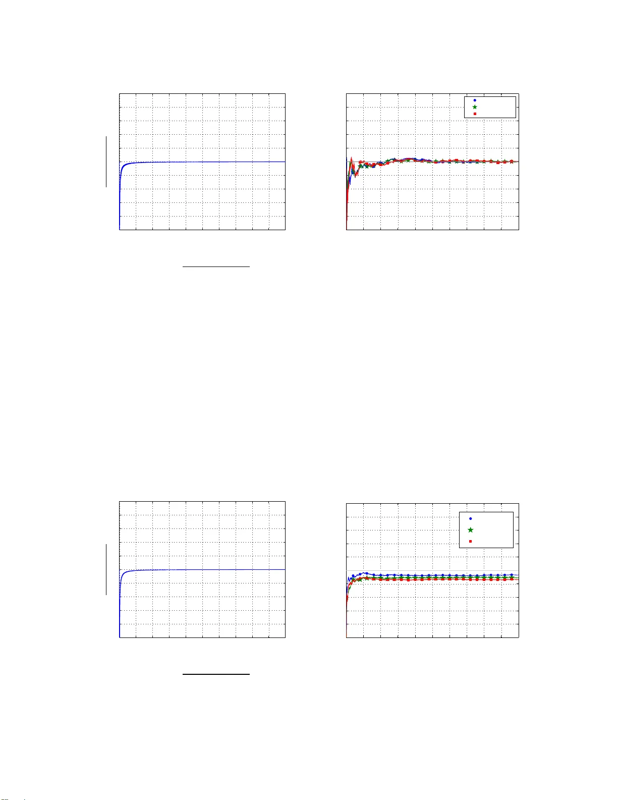
Authors: Dario Bauso, Puduru Viswanadha Reddy, Tamer Basar
1 L yapunov stochastic stability and control of rob ust dynamic c oalitional games with transferable utilit ies Dario Bauso, P . V iswanadha Reddy , T amer Bas ¸ ar , Abstract This paper con siders a dyn amic game with transferable utilities (TU), where th e characteristic function is a continuous-time bounded mean er go dic process. A central planner interacts continuously over time with the play ers by cho osing the in stantaneous allocatio ns subject to budget constraints. Before the game starts, the central plan ner knows the n ature o f the pro cess ( bound ed mean ergod ic), the bo unded set from which the co alitions’ values ar e sam pled, and the long r un average coalitions’ values. On th e o ther ha nd, he has no kn owledge of the u nderlyin g probab ility fun ction gener ating the coalitions’ values. Our g oal is to find allocation rules that use a measure of th e extra rew ard that a coalition has rece i ved up to the cu rrent time by r e-distributing the budget am ong the p layers. The ob jectiv e is two-fold : i) gu aranteeing convergence of the average alloca tions to th e co re (o r a specific point in the cor e) of the average game, ii) driving the coalitions’ excesses to an a prio ri given cone. The resulting allocatio n r ules are r obust as they gu arantee th e afore mentioned convergence proper ties d espite the uncerta in and time-varying nature of the coaltions’ values. W e highligh t three main co ntributions. First, we design an allo cation rule based on full o bservation of the extra rew ard so that the average a llocation ap proach es a sp ecific point in the core of the av erag e game, while the coa litions’ excesses co n verge to an a p riori g iv en d irection. Second, we design a new allocation rule b ased on par tial o bservation on the extra reward so that the av erag e allocation co n verges to th e Preliminary conference versions of this work were presented in Allerton 2010 [5] and C DC 2010 [6]. T he authors would like t o thank Ehud Leher and Eilon S olan for t heir support in exploring connections with approachability and attainability . D. Bauso is with Dipartimento di Ingegneria Chimica, Gestionale, Informatica e Meccanica, Universit ` a di Palermo, It aly , email: dario.bauso@un ipa.it P .V . Reddy is wi th GERAD and HEC Montreal, email: viswanad ha.puduru@gmail.com T . Bas ¸ ar is wit h Coordinated Science Laboratory , Univ ersity of Il linois at Urbana-Champaign, Urbana, IL, USA, e-mail: basar1@illinois.edu October 25, 2018 DRAFT 2 core of the average ga me, while the coalitio ns’ excesses conver ge to an a priori given co ne. And third, we establish con nections to appro achability theo ry [ 9], [18] and a ttainability theor y [4], [19]. Keyw ords Coalitional games wit h transferable utiliti es; allocation processes; approacha- bility theory; L yapunov stochastic stabili ty . I . I N T R O D U C T I O N Coalitional games with transferable ut ilities (TU), introduced first by V on Neuman and Morgenstern [25], have recently sparked much interest in the control and commu nication engineering communities [21]. I n essence, coalitional TU games are comprised of a set of players who can form coalitions and a characteristic fun ction associatin g a real number with e very coali tion. This real n umber represents the value of the coalition and can be thoug ht of as a monetary value that can be distributed among the m embers of th e coalition according to some appropriate fairness allocation rule. The v alue of a coalition als o reflects the monetary benefit demanded by a coaliti on to be a part of the grand coalit ion. This paper considers a dynamic TU g ame , where the characteristic function is a bounded mean ergodic process. Bounded means that t he characteristic function t akes values in a con ve x set according to an unknown probability distribution. M ean er godic means that the expected value of the coalitions values at each tim e coincides wit h the long t erm ave rage. W ith the dynamic g ame we asso ciate a dynamic average g ame obtained by av eraging over ti me the coalitions’ values, and assum e that the core of the average g ame is nonempt y on the long run. Giv en the above dynamic T U game, a central planner i nteracts conti nuously over time wi th the players by choosing t he in stantaneous allocations subject to budget constraints. Before the gam e starts, the central p lanner knows the nature of t he process (bounded mean ergodic), the bounded set and th e long run average coalitions’ values. On th e o ther hand, he has no knowledge of the und erlying probabil ity function generating the instantaneous coalition s’ values. Our goal is to find allocation rules that use a measure of the extra re ward that a coalition h as recei ved up t o t he current ti me b y re-distri buting t he budget am ong the p layers. The objectiv e is two-fold: i) guaranteeing con vergence of the a verage all ocations to the core (or a s pecific p oint in the core) of the a verage game, ii) driving the coalitio ns’ excesses to an a priori giv en cone. The resul ting allocation rules are rob ust as th ey guarantee t he aforementioned con ver gence properties despite the uncertain and tim e-v arying nature of the coaltions’ values. October 25, 2018 DRAFT 3 In the context of coali tional TU games, r obustness and dynamics natu rally arise i n all the situations where the coaliti ons values are u ncertain and time-varying, see e.g., [7]. Robustness has to do wi th modeling coaliti ons’ values as u nknown entities and this is in s pirit with some literature on stochasti c coalitional games [23], [24]. Ho weve r , we deviate from the latter works since t he probabilit y fun ction generating the random coalitions values is unknown, and this is more in line with the concept of Unknown But Bounded (UBB) variables formali zed in [8]. It is worth to m ention that this formulatio n shares som e comm on elements with the recent literature on interval valued games [1], where the authors use i nterva ls to describe coalitions values quite sim ilar to what is done in thi s paper . Th e i nterval nature of coalitions’ values arises g enerally due to the optimis tic and pessim istic expectations of t he coalit ions [11] when cooperation i s achiev ed from a strategic form game. W e also n ote some diffe rences in that we focus here more on the t ime-varying nature of the coali tions’ values. In doing so, we also link the approach to the set in var iance theory [10] and stochastic stability theory [20] which provides us some n ice tools for stabili ty analysis (see, e.g., the use of a L yapunov function in the proof of Th eorem 4.1). Bringing dynami cal aspects i nto the framew ork of coali tional TU games is an element in common with other papers [13], [16], [17]. The main difference with those works is that the values of coalitions are realized exogenously and no relation exists between consecutive samples. Con ver gence cond itions to gether with the idea that allocation rules use a measure of the extra rewa rd t hat a coalitio n has recei ved up to t he current time b y re-dist ributing the budget among the players are a main issue in a number of other papers [2], [12], [15], [18], [22] as well. Howe ver , this paper departs from th e aforementioned ones mainly in that dynamics in those works is capt ured by a bargaining mechanism with fixed coalition s’ values while we let t he values be time-varying and uncertain. This last element adds som e robustness to o ur allocation rule which has not been dealt with before. The main contribution of thi s paper is captured by the following th ree results. First, we design an allocation rule based on full ob serv ation of t he extra rew ard so t hat the ave rage allocation approaches a specific p oint in the core of the av erage g ame, while th e coalitions’ excesses con ver ge to an a prio ri given direction. Second, we design a new allocation rule based on partial observation on the extra re ward so t hat the average all ocation con ver ges October 25, 2018 DRAFT 4 to the core of th e average gam e, while the coalit ions’ e xcesses con ver ge to an a priori giv en cone. Con v ergence of bot h all ocation rules is proved vi a L yapunov sto chastic st ability theory . An d th ird, we establish connections of the L yapunov stochastic stabili ty theory to the approachability theory [9], [18] and at tainability theory [4], [19]. A few other contributions of t he paper are the definit ion of a verage game, whose role becomes fundamental when t he coalitions’ va lues variations are known with delay by the planner; the reformulat ion of the problem as a network flow control problem , where the allocation rule turns into a robust cont rol policy is a novel aspect, with the im portance o f such a reformulation l ying in t he fact that we can prove the con ver gence of the allocations using the s trong tools of the L yapunov stochastic stabilit y theory; and finally , the idea of turning a coali tional TU game set up into a cont rol theoretic probl em is a n ovel on e, which represents, by far , the main characteristics of this work. The paper is organized as follows. In Section II, we formu late the problem. In Section III, we present the basic i dea of our solution approach. In Section IV we state the t hree main results of this work and postpone the deriv ation o f such results to Section V. In Section VI, we provide some numerical i llustrations . Finally , in Section VII, we draw so me concluding remarks. Notation . W e view vectors as col umns. For a vector x , we u se x i or [ x ] i to denote i ts i th coordinate comp onent. For two vectors x and y , we use x < y ( x ≤ y ) to denote x i < y i ( x i ≤ y i ) for all coordinate indices i . W e let x T denote the transpose of a vector x , and k x k n denote i ts n -norm . For a m atrix A , we use a ij or [ A ] ij to denote i ts ij th entry . W e u se | a ij | to denote t he absolut e value of scalar a ij . Given two sets U and S , we write U ⊂ S to denote that U is a proper subset of S . W e u se | S | for t he cardinalit y of a g iv en finite set S . Let Φ be a cl osed and con vex set in R m , we use P ( y ) to denote t he projection of any point y ∈ R m onto Φ (closest point to y in Φ ). W e also denote by ∂ Φ the bo undary of Φ and n y the outward normal for any y ∈ ∂ Φ . W e use dist ( y , Φ) to deno te t he euclidean distance between point y and set Φ . Gi ven a s et N of players and a fun ction η : S 7→ R defined for each nonempty coalition S ⊆ N , we write < N , η > to denote the transferable utility (TU) g ame with the players’ set N and the characteristic function η . W e let η S be the value η ( S ) of the characteristic function η associated with a nonempt y coali tion S ⊆ N . Given a TU game < N , η > , we use C ( η ) to d enote the core of the g ame, C ( η ) = October 25, 2018 DRAFT 5 n x ∈ R | N | P i ∈ N x i = η N , P i ∈ S x i ≥ η S for all nonempty S ⊂ N o . Als o, R + denotes the set of n onnegati ve real numbers. Giv en a random vector ξ the notation E [ ξ ] denotes its expected value. Giv en a random process { v ( t ) } we denot e by ˜ v ( t ) = R t 0 v ( τ ) dτ , it s in tegral and ¯ v ( t ) = ˜ v ( t ) t its av erage up to tim e t . I I . M O D E L A N D P RO B L E M F O R M U L A T I O N In this section, we formul ate the problem in its generic form and elaborate on the rol e of information. L et N = { 1 , . . . , n } be a set of pl ayers and S ⊆ N the set of all (nonempty) coalitions arising among these players. Denote by m = 2 n − 1 th e number of possible coalitions . W e assume that tim e is continuous and use t ∈ R + to index t he time slots . W e consid er a dynamic TU g ame , denoted < N , { v ( t ) } > , where { v ( t ) } is a continuo us flo w of characteristic functions. The flow { v ( t ) } describes a bounded mean ergodic process. By b ounded we m ean that given a bounded con vex set V ∈ R m and a probability fun ction P ∈ ∆( V ) , wh ere ∆( V ) is the s et of probabili ty funct ions on V , then for all t ∈ R + each random v ariable v ( t ) takes values in V ∈ R m according to probabilit y P as expressed in (1); by mean er godic we mean t hat its expected v alue coin cides with t he long t erm avera ge as in (2): v ( t ) ∈ V ⊂ R m , for all t ∈ R + (1) E [ v ( t )] = l im τ → ∞ ¯ v ( τ ) , for all t ∈ R + . (2) Thus, in the dynamic TU gam e < N , { v ( t ) } > , t he players are in volved in a sequence of instantaneous TU games whereby , at each time t , the inst antaneous TU game i s < N , v ( t ) > with v ( t ) ∈ V for all t ≥ 0 . Further , we let v S ( t ) denote the value a ssigned to a nonempt y coalition S ⊆ N in th e instantaneous game < N , v ( t ) > . W it h the dynami c game we associate a dynam ic avera ge game < N , { ¯ v ( t ) } > and an instantan eous average game at t ime t ≥ 0 , < N , ¯ v ( t ) > . The mot iv ation of formalizing t he above dynamic TU games is in that such games represent a stylized model of all tho se scenarios where the coalition s’ values v ary with ti me. W e assum e that the core of th e ave rage game is nonempt y on the long run. W e will see that w ithout this assum ption th e p roblem under study has no s olution. Thus, denote by v nom the (long run) average coalitions ’ values, nam ely , v nom := lim t →∞ ¯ v ( t ) and let C ( v nom ) be the core of the av erage game. October 25, 2018 DRAFT 6 Assumption 1: (balancedness) The core of the avera ge game is nonempty in the limi t: C ( v nom ) 6 = ∅ . W e can view the abov e assum ption as introducing som e steady-state (a verage) condit ions on a game scenario subject to ins tantaneous fluctuati ons. Howe ver , note that we do not make assumption s regarding t he balancedness of the inst antaneous gam es which is t he case wit h [7]. Thus, the core of t he instantaneous game can be empty at som e time t . Giv en the above dynamic TU game, a central planner interacts continuousl y over t ime with the pl ayers by choosing t he inst antaneous allocation s denoted by a ( t ) ∈ R n . W e assume that the allocations are subj ect to the following budget constraints. Assumption 2: (bounded allocation) The in stantaneous allocation is bounded within a hyperbox in R n a ( t ) ∈ A := { a ∈ R n : a min ≤ a ≤ a max } , with a prior i given lower and u pper bounds a min , a max ∈ R n . As regards the i nformation a vailable a priori (before t he game starts) to the central planner , we assume that he knows the natu re of the process { v ( t )) } (bo unded mean er godi c), the bounded s et V and the long run av erage coalitions’ values v nom . The l atter is the same as saying that he k nows the expected coali tions’ values for all t ∈ R + . On the other hand, he has no knowledge of the underlying probabilit y functi on P . Assumption 3: (on available information) The planner knows v nom . Beside th is, during the game the central plann er also observes the extra reward of t he coalitions u p to t and for all t ∈ R + . Given this, and in li ne with a number of other papers [2], [12], [15], [18], [22], our goal is to find allo cation rules that use a measure of the extra re ward t hat a coalition has receiv ed up to the current time by re-distributing the budget am ong the players. T o do this , a first step is t o define excesses for the coalitions . For any coaliti on S ⊆ N , we define excess (extr a re war d) at time t ≥ 0 as the e xcess at time t = 0 plus the diffe rence between the total integral rew ard, given to it, and th e int egral value of the coalition itself, i.e., ǫ S ( t ) = X i ∈ S ˜ a i ( t ) − ˜ v S ( t ) + ǫ S (0) . Furthermore, assumi ng without loss o f generality ǫ S (0) = 0 , we say that S is in excess at time t ≥ 0 if the excess is nonnegati ve, i.e., P i ∈ S ˜ a i ( t ) ≥ ˜ v S ( t ) . Let ǫ ( t ) represent the vector October 25, 2018 DRAFT 7 of coalitions’ excesses, formally giv en as: ǫ ( t ) = { ǫ S ( t ) } N ⊇ S 6 = ∅ . W e are interested in answering two main quest ions for this class of games. • Question 1: Are th ere all ocation rules such that t he avera ge allocatio ns con ver ge? If yes, let us denote by A 0 the set where the ave rage all ocations con verge to . Can we make it conv erge to the core of the av erage gam e A 0 ⊆ C ( v nom ) ? Can we guarantee the con vergence to a specific poi nt of the core, call it nom inal allocation a nom , th at we have a priori selected? • Question 2 : Are there all ocation rules such t hat the coalitions’ excesses ǫ ( t ) con ver ge to an a prio ri given cone Σ 0 , say for i nstance the nonnegativ e m -dim ensional orthant R m + , or any direction αt for t ≥ 0 with fixed α ∈ R m + ? T o motiva te t he above questions think of a sit uation where the objective of the central planner is to maint ain the stability of g rand coalition i n an av erage sense, while controllin g the coalitions ’ excesses at each tim e t ∈ R + . W e are now in the position of providing a formal and generic statem ent of the problem. Henceforth, we use the symb ol w .p. 1 to mean “with probabil ity one”. Pr oblem 2 .1: Find an allocation rul e f : R m → A ∈ R n , such that if a ( t ) = f ( ǫ ( t )) then i) lim t →∞ ¯ a ( t ) ∈ A 0 ⊆ C ( v nom ) w .p.1, and ii) lim t →∞ ǫ ( t ) ∈ Σ 0 ⊆ R m + w .p.1. Observe that because of the random nat ure o f the coalit ions’ values v ( t ) , b oth t he excesses ǫ ( t ) and the allocations a ( t ) are random and as such we look at the con ver gence of ¯ a ( t ) w .p.1. Essentially , we require that the probability of ¯ a ( t ) con ver gin g in the lim it to A 0 ⊆ C ( v nom ) is 1 . Similarly for ǫ ( t ) and Σ 0 . This ty pe of con ver gence is also known as almos t sur e con vergence [20 ]. W e wil l show that if t he planner has full observation of ǫ ( t ) at ev ery tim e t then t he above problem is solvable eve n un der the very st rict condition of A 0 = a nom and Σ 0 = αt t ≥ 0 with fixed α . Con versely , if the plann er has partial observation of ǫ ( t ) in t hat he only knows the sign o f each component of ǫ ( t ) , then the problem is sti ll s olvable but under the relaxed condition of A 0 = C ( v nom ) and Σ 0 ⊆ R m + . October 25, 2018 DRAFT 8 A. Motivation s Dynamic coalitional games capture coordination in a number of network flow application s. Network flows model flow of goods, materials, or o ther resources between dif ferent produc- tion/dist ribution sites [3]. W e next provide a supply chain applicatio n th at justifies the m odel under study . A s ingle warehouse v 0 serves a number of retailers v i , i = 1 , . . . , n , each one facing a demand d i ( t ) unkn own but b ounded by pre-assigned values d min i ∈ R and d max i ∈ R at any time perio d t ≥ 0 . After demand d i ( t ) has been realized, retailer v i must choose to eit her fulfill th e dem and o r no t. The retailers do not h old any priv ate inv entory and, therefore, if they wish to fulfill their demands, they must reorder goods from the central warehouse. Retailers benefit from joint reorders as they may share the total transpo rtation cost K (this cost could also be ti me and/ or players dependent). In particular , if retailer v i “plays” individually , the cost o f reordering coincides wit h th e full transportation cos t K . Actually , when necessary a single truck wil l serve on ly him and get back to the warehouse. This is il lustrated b y the dashed cycles ( v 0 , v 8 , v 0 ) , ( v 0 , v 9 , v 0 ) , and ( v 0 , v 10 , v 0 ) in t he network of Figure 1. The cost of not reordering is the cost of the unfulfilled demand d i ( t ) . v 3 v 4 v 1 v 0 v 2 v 5 v 6 v 7 v 8 v 9 v 10 (a) Fiv e t rucks (cycles) leaving v 0 and serving coalitions { v 1 , . . . , v 4 } , { v 5 , . . . , v 7 } , { v 8 } , { v 9 } , and { v 10 } re- specti vely . v 3 v 4 v 1 v 0 v 2 v 5 v 6 v 7 v 8 v 9 v 10 (b) One single t ruck (cycle) leaving v 0 and serving coali- tion { v 1 , . . . , v 10 } . Fig. 1. Example of a distribution network If two or more retailers “play” in a coalition, they agree on a joint decision (“e veryone reorders” or “no o ne reorders”). The cost of reordering for the coalition also equals the total transportation cost that must be shared among t he retailers. In this case, when necessary a single truck will serve all retailers in the coalition and get back to the war ehouse. This is il - lustrated, with r eference to coalition { v 1 , . . . , v 4 } by the dashed c ycle ( v 0 , v 4 , v 1 , v 2 , v 3 , v 0 ) in October 25, 2018 DRAFT 9 Figure 1(a ). A similar comment applies to the coalition { v 5 , v 6 , v 7 } and the cycle ( v 0 , v 5 , v 6 , v 7 , v 0 ) in Figure 1(a). The network topolog y in Figure 1(a) describes th e existing coalitio ns. This is clear if we look at the subgraph induced by the vertex-set { v 1 , . . . , v 10 } (all ver tices except v 0 ) and observe that such a s ubgraph h as 5 connected com ponents, i.e., { v 1 , . . . , v 4 } , { v 5 , . . . , v 7 } , { v 8 } , { v 9 } , and { v 10 } and that each component corresponds to an existing coalition. The cost of not reordering is t he sum of the unful filled demands of all retailers. How the players will share the cost is a part of the solut ion generated by t he bar gainin g process. Con versely , the subgraph induced by { v 1 , . . . , v 10 } in Figure 1(b) has a sin gle connected component w hich m eans t hat all retailers “play” in the grand coalition and as such one s ingle truck (cycle) will l ea ve v 0 and serve all of t hem before returning to v 0 . Thi s is represented by the dashed cycle ( v 0 , v 4 , . . . , v 10 ) in the same figure. The cost scheme can be captured by a game with t he set N = { v 1 , . . . , v n } of players where the cost of a nonem pty coalition S ⊆ N is giv en by c S ( t ) = min ( K, X i ∈ S d i ( t ) ) . Note that the bounds on the demand d i ( t ) reflect into the bounds on th e cost as foll ows: for all nonempty S ⊆ N and t ≥ 0 , min ( X i ∈ S K, d min i ) ≤ c S ( t ) ≤ min ( K, X i ∈ S d max i ) . (3) T o complete t he deriv ation of the coalit ions’ values we need to compute t he cost savings v S ( t ) of a coalition S as the dif ference between the sum of the costs o f the coalition s of the individual players in S and the cost o f the coalition itself, namely , v S ( t ) = X i ∈ S c { i } ( t ) − c S ( t ) . Giv en the bou nd for c S ( t ) in (3), the value v S ( t ) is also b ounded, as given: for any S ⊂ N and t ≥ 0 , v S ( t ) ≤ X i ∈ S min { K, d max i } − min ( K, X i ∈ S d min i ) . Thus, the cost savings (v alue) of each coali tion is bounded uniformly by a maximum value. Introducing time asp ects into a static TU game opens th e possibility for mo deling aspects such as in tertemporal transfers, patience and expectations of players/coalition s. A g eneric October 25, 2018 DRAFT 10 dynamic coali tional g ame description shoul d capture these features. In a repeated j oint replen- ishment game as the one discus sed above, allocation rules ha ving the properties formal ized in Problem 2.1, encourage patient retailers to “play” in the grand coalition, to coordi nate their repleni shment policies and therefore t o reduce to tal t ransportation cost s. W e say patient retailers since condit ion i ) in Problem 2.1 guarantees conv ergence to core on the lo ng-run, i.e., in an ave rage sense. Condition ii) has the meaning of boundin g the excesses du ring the transient (before con ver gence occurs). I I I . F L O W T R A N S F O R M A T I O N BA S E D DY NA M I C S The basic idea of our soluti on approach i s to recast the p roblem into a flo w cont rol one. T o do this, consi der the hyper- graph H with vertex set V and edge set E as: H := { V , E } , V = { v 1 , . . . , v m } , E := { e 1 , . . . , e n } . Figure 2 depicts an example of hypergraph for a 3-player coaliti onal g ame. The ver tex set V has one vertex per each coalition whereas the edge set E has on e edg e p er each player . A v 1 v 2 v 3 v 4 v 5 v 6 v 7 e 1 e 3 e 2 Fig. 2. Hyperg raph H := { V , E } for a 3 -player coalitional game. generic edge i i s in cident to a verte x v j if the player i is in the coalition asso ciated to v j . So, incidence relations are described by m atrix B H whose rows are the characteristic vectors c S ∈ R n . W e recall that the components of a characteristic vector c S i = 1 if i ∈ S and c S i = 0 if i / ∈ S . The flo w control reformulation arises n aturally if we view allocation a i ( t ) as the flo w on edge e i and the coalition value v S ( t ) of a generic coaliti on S as the demand in the October 25, 2018 DRAFT 11 corresponding vertex v j . In view of this, allocation in th e core translates into over -satisfyi ng the demand at the vertices. Specifically , a ( t ) ∈ C ( v ( t )) ⇔ B H a ( t ) ≥ v ( t ) , (4) with the last inequality satisfied with the equal sign due to t he efficienc y condition o f t he core, i.e, P i =1 a i ( t ) = v m ( t ) , where v m ( t ) denotes the m t h compo nent of v ( t ) and is equal to t he grand coali tion value v N ( t ) . Now , s ince v ( t ) i s uno bserva ble by the pl anner at time t , we need t o int roduce som e allocation error dy namics wh ich accounts for the deriv at iv es of the excesses. Since ǫ ( t ) represents the coalition excess, we hav e: ˙ ǫ ( t ) = B H a ( t ) − v ( t ) , v ( t ) ∈ V . (5) Note th at the above d iff erential equ ation adm its a solut ion at least in the sense of Fili ppov [14]. From (4) and by averaging and taking the limit in (5), we can reformul ate Problem 2.1 as a flow con trol problem where a controller wishes to d riv e t he quantity lim t →∞ ǫ ( t ) − ǫ (0) t to the target set T , defined below , w .p.1 (see, e.g., Fig . 3): T := { τ ∈ R m : τ m = 0 , τ j ≥ 0 , ∀ j = 1 , . . . , m − 1 } . Note, τ m = 0 due to efficienc y of all ocations. τ m T ǫ ( t ) − ǫ (0) t Fig. 3. T rajectory for ǫ ( t ) − ǫ (0) t . October 25, 2018 DRAFT 12 Remark 3.1: Driving the a verage allocations to a particul ar point a nom ∈ A 0 ⊆ C ( v nom ) re- sults in reaching a s pecific poin t in the target set T . T o see thi s, note that w hen lim t →∞ ¯ a ( t ) = a nom we hav e T ∋ B H a nom − v nom ≥ 0 due to th e property of the core. Thus, we als o ha ve that lim t →∞ ǫ ( t ) − ǫ (0) t is driven t o the point B H a nom − v nom ∈ T . The i nequality condit ion in (4 ) is transformed into equalit y type by i ntroducing, from standard LP techniq ues, m − 1 surplu s variables (one per each coalition other than the grand coaliti on). This increases the d imension o f the cont rol space of the planner from m to n + m − 1 and the dynamics (5) can be rewritten as follows: ˙ x ( t ) = B u ( t ) − v ( t ) , v ( t ) ∈ V (6) where B = B H − I m − 1 0 ∈ R m × n + m − 1 . V ariable x ( t ) represents the state of the s ystem and captures deviation from the balanced system, i.e., the system characterized b y a nom and v nom . W e introdu ce t he set of feasible controls as: U := u ( t ) ∈ R n + m − 1 : u ( t ) = [ a T ( t ) s T ( t )] T , a ( t ) ∈ A , s ( t ) ≥ 0 . (7) T ow ard the reformulation o f the problem as a stochasti c stabilizabili ty one, we introduce the following prelimi nary result. Lemma 3.1: If t he variable x ( t ) is asymptoticall y sta ble al most sur ely , i .e., (8) holds true, then the av erage al locations con verge to t he core of t he av erage game w .p.1. as expressed by (9), and the excesses con verge to the cone R m + w .p.1. as described in (10): lim t →∞ x ( t ) = 0 , w .p.1 . (8) lim t →∞ ¯ a ( t ) ∈ C ( v nom ) , w .p.1 (9) lim t →∞ ǫ ( t ) ∈ R m + , w .p.1 . (10) Pr oof: T o see why (8) implies (9), observe that if lim t →∞ x ( t ) = 0 w .p.1 . then lim t →∞ x ( t ) − x (0) t = 0 w .p.1. and therefore, by integrating and dividing b y t i n (6) als o lim t →∞ B ¯ u ( t ) − ¯ v ( t ) = 0 w .p.1. The latter can be rewritten as lim t →∞ B ¯ u ( t ) = v nom w .p.1, and as from (7) ¯ s ( t ) = B H ¯ a ( t ) − ¯ v ( t ) ≥ 0 and v nom is balanced by Assumption 2 then we conclude that lim t →∞ ¯ a ( t ) ∈ C ( v nom ) w .p .1. T o see why (8) implies (10), observe that if lim t →∞ x ( t ) = 0 w .p.1., from (7) and under the assumpt ion x (0) = ǫ (0) = 0 , then lim t →∞ ǫ ( t ) = lim t →∞ ˜ s ( t ) ≥ 0 and (10) is proved. October 25, 2018 DRAFT 13 It i s worth noting that condi tion (9) is part of Problem 2.1. In oth er words when solv ing Problem 2.1 we always guarantee (9). If t his is clear then, we can use th e above lemma to rephrase Problem 2.1. In do ing t his we need to make a partial d istinction between cases i) and ii). More specifically , case ii) where A 0 = C ( v nom ) can be restated as follows: Find u ( t ) := φ ( x ( t )) ∈ U s uch that lim t →∞ x ( t ) = 0 w .p.1. (11) Note that if we wish to reach a s pecific point a nom then the cond ition (9) is onl y necessary and the resulting problem is a st ricter version of (11). I V . M A I N R E S U LT S In thi s section we p resent the t hree main results of this work. The first one relates to the case where t he planner has full observation on x ( t ) in which case the av erage allo cation can be dri ven to a specific point i n the Core of the av erage game. The second result applies to t he case wh ere the planner has partial observation on x ( t ) , and con ver gence to the Core can sti ll be guaranteed but not to a sp ecific point of the Core. The thi rd result highlight s connections of th e implemented solut ion approach to the approachabili ty principle [9], [18] and attainabili ty pri nciple [4], [19]. A. Full infor mation case In this section, we s olve Problem 2.1 wit h A 0 = a nom and Σ 0 = α t, t ≥ 0 with fixed α under the assum ption th at the planner has full obs erv ation of t he exce sses ǫ ( t ) and therefore x ( t ) as well. W e recall th at inferring x ( t ) from ǫ ( t ) is possible as the s urplus s ( t ) is selected by the planner . As we have said before, the p roblem that we solve i s a stri cter version o f (11). This version derives from aug menting the state of dynami cs (6) as explained i n the rest of this section. Before in troducing the augment ation technique let us assume that the fluctuations of the coalitions’ v alues around the mean v nom are independent of the state x ( t ) . W e formalize this in th e next assum ption where we denote by ∆ v ( t ) = v ( t ) − v nom the above fluctuations. Assumption 4: The s tate x ( t ) and th e coalitions ’ va lues fluctuati ons ∆ v ( t ) are i ndependent. Introducing the fluctuations ∆ v ( t ) allows us to rewr it e dynamics (6) in a more con venient way . T o do this, note first th at, as u ( t ) = [ a ( t ) T s ( t ) T ] T and from B u nom = v nom , if a nom is fixed then s nom ∈ R m − 1 + and therefore also u nom = [ a T nom s T nom ] T are fixed. L et us d enote October 25, 2018 DRAFT 14 ∆ u ( t ) = u ( t ) − u nom . Dynamics (6) can be rewritten as follows: ˙ x ( t ) = B u ( t ) − v ( t ) = B u ( t ) − ( v nom + ( v ( t ) − v nom )) = B u ( t ) − v nom − ∆ v ( t ) = B ( u ( t ) − u nom ) − ∆ v ( t ) = B ∆ u ( t ) − ∆ v ( t ) W e mentioned before that we will focus on a stricter version of (11). W e do this by augmenti ng the state as sho wn next. F irst, d enote by B † a generic pseudo in verse matrix of B and com plete matrices B and B † with matrices C and F such that B C h B † F i = I . (12) Then, building upon the n e w s quare matrix B C , let us consider the augmented syst em ˙ x ( t ) = B ∆ u ( t ) − ∆ v ( t ) ˙ y ( t ) = C ∆ u ( t ) . (13) Here we assume that v ( t ) is i ndependent of y ( t ) as well. After integrating the above system (see (14), right) we define a new variable z ( t ) as follows: z ( t ) = h B † F i x ( t ) y ( t ) , x ( t ) y ( t ) = B C z ( t ) . (14) It turns out that to driv e x ( t ) t o zero w .p.1, and obtain u nom as av erage allocation on the long run, we can rely on a simple function ˆ φ ( . ) , which depends on z ( t ) . Before introd ucing this functio n, for future purpo ses observe that t he dynami cs for z ( t ) sati sfies the first-order diffe rential equatio n: ˙ z ( t ) = h B † F i ˙ x ( t ) ˙ y ( t ) = h B † F i B C ∆ u ( t ) − h B † F i ∆ v ( t ) 0 = ∆ u ( t ) − B † ∆ v ( t ) . (15) Let ∆ u min and ∆ u max be the m inimal and maxim al v alues of ∆ u ( t ) for the following constraints to hold true: u ( t ) = u nom + ∆ u ( t ) ∈ U . Then, let us formal ly d efine ˆ φ ( z ( t )) October 25, 2018 DRAFT 15 ˙ x ( t ) = B ∆ u ( t ) − ∆ v ( t ) ˙ y ( t ) = C ∆ u ( t ) v ( t ) u ( t ) ˆ φ ( z ( t )) z ( t ) = h B † F i x ( t ) y ( t ) Fig. 4. Dynamical System as: ˆ φ ( z ( t )) := u nom + ∆ u ( t ) ∈ U, ∆ u ( t ) = sat [∆ u min , ∆ u max ] ( − z ( t )) , (16) where with sat [ a,b ] ( ξ ) we denote the saturated functio n th at, given a generic vector ξ and lower and upper bo unds a and b of same dim ensions as ξ , retu rns sat [ a,b ] ( ξ ) . = b i for all i ξ i > b i a i for all i ξ i < a i ξ i for all i a i ≤ ξ i ≤ b i . Now , t aking the control u ( t ) = ˆ φ ( z ( t )) , we obtain the dynami c system ˙ z ( t ) = B ˆ φ ( z ( t )) − v ( t ) as displayed in Fig. 4 . W ith the above preambl e in min d, we are ready to state the following con vergence pro perty . Theor em 4.1: Using the cont roller ˆ φ ( z ( t )) , as in (16), we h a ve lim t →∞ z ( t ) = 0 w .p .1 and therefore lim t →∞ ¯ u ( t ) = u nom . In the next corollary , we use the previous result to provide an answer t o Problem 2.1. Cor ol lary 4 .1: The state x ( t ) is driven to zero w .p .1 as expressed in (11), the a verage allocation con ver ges to the nominal allocation i.e., lim t →∞ ¯ a ( t ) = a nom , w .p.1 and the e xcesses con verge to the direction Σ 0 = αt with α = s nom , i.e., lim t →∞ ǫ ( t ) ∈ Σ 0 . Pr oof: This is a direct consequence of the result proved in the previous theorem. From (14), and [ B † F ] being a n on singu lar matrix, we hav e lim t →∞ x ( t ) = 0 w .p .1. From th e October 25, 2018 DRAFT 16 pre viou s theorem we als o have lim t →∞ ¯ u ( t ) = u nom . Since u ( t ) = [ a T ( t ) s T ( t )] T , we ha ve that lim t →∞ ¯ a ( t ) = a nom and lim t →∞ ǫ ( t ) = ˜ s ( t ) = s nom t . T o summarize, in the full information case, the control ler u ( t ) defined by (16) indu ces an allocation sequence a ( t ) such that the aver age ¯ a ( t ) conv erges to A 0 = a nom and th e excesses approach s nom t . B. P artia l in formation case In th e previous section w e observed that if the planner has full observation of th e excesses and therefore of x ( t ) then he can d esign an allocation rule so that the ave rage allocations are driv en to a nom and the excesses approach s nom t . In this s ection, we solve Problem 2.1 with A 0 = C ( v nom ) and under the ass umption that th e planner has partial ob serv ation of x ( t ) . In particul ar , we assume that the planner o bserves the sign of x ( t ) for all t ∈ R + . An information s tructure based on t he sign of x ( t ) h as an oracle-based interpretation which we discuss in detail in Subsectio n IV -B1. Similarly to the previous section, suppose t hat we know a particular allocation a nom in the core C ( v nom ) , and l et us stud y the con ver gence properties of the av erage allocations . In parti cular , using an allocati on rule u ( t ) = φ ( x ( t )) , we require that x ( t ) sati sfying the dynamics ˙ x ( t ) = B φ ( x ( t )) − v ( t ) , con ver ge to zero in probabilit y . In this secti on, we state the second main resul t of this work which provides a s olution to Problem 2 .1 with p artial information structure. T o do this, let us denote again by B † a generic pseudo in verse m atrix of B and t ake a feasible allocation u nom such that B u nom = v nom := lim t →∞ ¯ v ( t ) , u nom ∈ U. Also, for future purposes, define a function ˆ φ ( . ) , which depends only on the sign of x ( t ) , as follows: ˆ φ ( sg n ( x ( t ))) := u nom + ∆ u ( t ) ∈ U, ∆ u ( t ) = − δ B † sg n ( x ( t )) . (17) Now , t aking t he control u ( t ) = ˆ φ ( sg n ( x ( t ))) , we obtain the dynamic system ˙ x ( t ) = B ˆ φ ( sg n ( x ( t ))) − v ( t ) as displayed in Fig. 5. Now , we state th e following con ver gence property . Theor em 4.2: Using the c ontrol ler u ( t ) = ˆ φ ( sg n ( x ( t ))) as in (17) we ha ve lim t →∞ x ( t ) = 0 w .p.1. Cor ol lary 4 .2: The av erage allocation con ver ges to the core of the avera ge game as in (9) and the excesses ǫ ( t ) con verge to R m + as in (10). October 25, 2018 DRAFT 17 ˙ x ( t ) = B ∆ u ( t ) − ∆ v ( t ) v ( t ) u ( t ) ˆ φ ( sgn ( x ( t ))) sgn ( x ( t )) Fig. 5. Dynamical System Pr oof: Direct consequence of Theorem 4.2 and Lemm a 3.1. 1) Oracle-based interpr etati on: In this subsection we elaborate m ore on the partial infor- mation structure. In particular , we highlight ho w the feedback on state x ( t ) can be re viewed as t he result of an oracle-based procedure. T o see this, assu me that the planner knows the sign of x ( t ) . Since x ( t ) = ( ǫ ( t ) − ˜ s ( t )) − ( ǫ (0) − x (0)) , sgn ( x ( t )) reflects over -satisfaction of coalit ions with respect to the threshold ˜ s ( t ) . In particular , t ake witho ut loss of generality ǫ (0) , x (0) = 0 , then with reference to comp onent j , the sign of x j ( t ) yields: sg n ( x j ( t )) := 1 ǫ j ( t ) > ˜ s j ( t ) 0 ǫ j ( t ) = ˜ s j ( t ) − 1 ǫ j ( t ) < ˜ s j ( t ) . (18) T o summarize, we can think of a sit uation where the planner approaches an oracle that tells him th e sign of x ( t ) . Since s ( t ) is chosen by the planner for ev ery t , the accumulated surplus, ˜ s ( t ) , is given as an inpu t t o the oracle. Th e oracle returns “yes” if the actual excess is greater than ˜ s ( t ) and “no ” ot herwise. The use of an oracle is an element in commo n with t he ell ipsoid method in optimi zation and wit h a large literature [26 ] on cutting planes. Recall that nonnegativ eness of the thresh old has i ts roots in the feasibil ity condi tion u ( t ) ∈ U for all t ≥ 0 with feasible set U as in (7). Nonnegativ eness of t he threshold provides u s wit h a further comment on t he information a vailable to the p lanner . Actually , from the first condition in (18), we can conclude that coalitions associated to a positive state x ( t ) are certainly in excess. This is clear if we observe that sg n ( x j ( t )) = 1 im plies ǫ j ( t ) > ˜ s j ( t ) ≥ 0 . W e can then sum marize the in formation October 25, 2018 DRAFT 18 content av ailable to the planner as follows, where S is the generic coaliti on associated wi th component j : sg n ( x j ( t )) := 1 then coalition S in excess − 1 , 0 nothing can be said . T rivially , the dev elopment in the full inform ation case in Section IV -A , which is all based on control strategy (16), fits the case where x ( t ) is revealed completely . In t his last case, the fact t hat the planner kn ows x ( t ) implies that he knows ǫ ( t ) as well. Als o, it is int uitive to infer th at in this last s et up, exact knowledge of x ( t ) can only i nfluence posit iv ely the planner in terms of speed of con vergence of all ocations to the core of the ave rage game. Remark 4.1: As the planner knows a priori th e no minal g ame and a corresponding nominal allocation vector , a natu ral question that arises is why one has to desi gn an allocation rule as give n b y (16) and (17) ins tead of a st ationary rul e ˆ φ ( . ) = u nom . The rul es give n b y (16) and (17) intuitively t ranslate to meeting the demands of coalitions in an av erage sense. Th is feature reflects patience aspect of coali tions in a dynam ic setti ng, i. e., even if a demand is not met instantaneous ly a coalition is wi lling to wait and stay in the grand coali tion as the demand is fulfilled in an aver age sens e. C. Connections to Approac habili ty and Att ainabilit y 1) Appr oa chability: Approachability theory was deve loped by Blackwell in 1956 [9] and is captu red in the well known Blackwell’ s T heorem. Alo ng the lines of Section 3.2 in [18 ], we recall next the geometric (approachability) p rinciple that l ies behind Blackwell’ s Theorem. The goal of this section i s t o sh ow that such a geometric principle sh ares striking sim ilarities with the solut ion approach used in the pre viou s sections. T o introd uce the approachability principle, let Φ be a closed and conv ex set in R m and let P ( y ) be the projection of any point y ∈ R m (closest point to y in Φ ). Also denot e by ¯ y k the a verage of y 1 . . . , y k , i.e., ¯ y k = P k t =0 y t k and let dist ( ¯ y k , Φ) be the euclidean distance between point ¯ y k and set Φ . Lemma 4.1: (Approachability principle [18]) S uppo se that a s equence of uniformly bou nded vectors y k in R m satisfies condition (19), [ ¯ y k − P ( ¯ y k )] T [ y k +1 − P ( ¯ y k )] ≤ 0 , (19) then lim k →∞ dist ( ¯ y k , Φ) = 0 . October 25, 2018 DRAFT 19 Now , t o make us e o f the above princip le in ou r set up, let us consider the di screte t ime analog of the excess dynamics (6): x k +1 = x k + B ∆ u k − ∆ v k , and define a new v ariable y k = x k − x k − 1 so that we can look at the sequence of y k in R m . Like wise, consider the dis crete t ime version of control (17) as displayed below: ˆ φ ( sg n ( x k )) := u nom + ∆ u k ∈ U, ∆ u k = − δ B † sg n ( x k − x 0 ) . (20) W e are now in a position to state the main result of t his section. Theor em 4.3: Using the controller u k = ˆ φ ( sg n ( x k − x 0 )) as in (20) we h a ve that i) the vector 0 is approachable by the sequence ¯ y k , lim k →∞ ¯ y k = 0 , w . p.1 , (21) and therefore ii) t he a verage allocations con ver ge to the core of t he a verage game, lim k →∞ ¯ a k ∈ C ( v nom ) , w .p.1 . (22) The strength of t he above result is in that it sheds lig ht on how the con ver gence probl em dealt wi th in th is work has a stochastic st ability i nterpretation as well as an approachability one. Remark 4.2: (Continuous-tim e approachability) W e can reformul ate Theorem 4.3 in the continuous time. T o see thi s, l et us first define y ( t ) := ˙ x ( t ) . Next we need to deriv e the continuous time version of (19). T o t his aim, let t → r ( t ) be a differentiable contin uous tim e var iable and let z ( t ) = r ( t ) − r (0) t , so t ˙ z ( t ) + z ( t ) = ˙ r ( t ) . Discrete time versions are given as z k = 1 k r k and z k +1 = 1 k +1 r k +1 . The approachability principle is given as [ z k − P ( z k )] T [ φ − P ( z k )] ≤ 0 where φ = ( k + 1) z k +1 − k z k . In continu ous t ime the above condition translates to [ z ( t ) − P ( z ( t ))] T [ φ − P ( z ( t ))] ≤ 0 and φ = ( t + ∆ t ) z ( t + ∆ t ) − tz ( t ) = t ( z ( t + ∆ t ) − z ( t )) + ∆ tz ( t + ∆ t ) . W e see that φ ∆ t = t z ( t +∆ t ) − z ( t ) ∆ t + z ( t + ∆ t ) . Further , as ∆ t → 0 w e have lim ∆ t → 0 φ ∆ t = t ˙ z ( t ) + z ( t ) = ˙ r ( t ) . The approachability principle in conti nuous time can then be reproposed as [ z ( t ) − P ( z ( t ))] T [ ˙ r ( t ) − P ( z ( t ))] ≤ 0 , (23) October 25, 2018 DRAFT 20 which constitut es the continuou s time version of (19). If Φ = { 0 } we have P ( z ( t )) = 0 and z T ( t ) ˙ r ( t ) ≤ 0 . Now , t aking r ( t ) = x ( t ) we see that z ( t ) is the average of y ( t ) . T hen condition (23) guarantees that z ( t ) conv erges to zero as well as ¯ y ( t ) . But this i mplies that lim t →∞ x ( t ) − x (0) t = 0 and t herefore from L emma 3.1 we arriv e at (9) wh ich represents t he continuous time version of (22). 2) Attainabilit y: Attainabil ity is a ne w notio n deve lop ed in [4], [19] in the context of 2-player conti nuous-time repeated games with vector payof fs. At tainability finds i ts roots in transportation networks, distribution networks, production networks applications. The main question i s the following o ne: “Under what cond itions a strategy for player 1 exists s uch th at the cumulative payoff con ver ges (in the lim sup sense) to a pre-assigned set (in the space of vector payoffs) independently of the strategy used by player 2”. Attainabilit y shares similarities with two m ain noti ons i n rob ust control theory [10]. The first notion is called rob ust global a ttractiveness and refers to the property of a set to “attract” the state of th e system under a proper control strategy and i ndependently of t he ef fects of the disturbance. The second not ion is referred to as rob ustly controlled i n var iance and describes th e property of a set t o bound the s tate trajectory u nder a proper control strategy and ind ependently of the ef fects of the disturbance. Both n otions are used in the following formalization of the attainabilit y principle. The principl e is accomp anied by a sketch of the proof but no formal proof i s reported as attainabil ity is the main focus of anot her paper and here it is just auxiliary to t he solution of our main prob lem and also because the aforementioned two noti ons are well k nown in robust control theory . W e refer the readers to [10] and [4], [19] for further detail s. Let Φ be a clo sed and con vex set in R m and consider a di f ferentiable continuous -time var iable t 7→ y ( t ) taking value i n R m for all t ≥ 0 . Lemma 4.2: (Attainability principl e [4], [19]) Suppose t hat the differentiable cont inuous- time variable t 7→ y ( t ) satisfies conditio ns (24)-(25), [ y ( t ) − P ( y ( t ))] T [ ˙ y ( t ) − P ( y ( t ))] < 0 , y ( t ) 6∈ Φ (24) n T y ( t ) [ ˙ y ( t ) − P ( y ( t ))] ≤ 0 , y ( t ) ∈ ∂ Φ , (25) then lim t →∞ dist ( y ( t ) , Φ) = 0 . Essentially , conditio n (25) is strictly related to t he subtan gentiality conditions as formulated by Nagumo in 19 42 and s urveye d in [10]. Such conditio ns are proven to characterize robustly October 25, 2018 DRAFT 21 controlled i n variant s ets. W e p rovide a geom etric perspective on such a condi tion in Fig . 7(b). Consider a 2 player continuous-time repeated game and let y ( t ) be t he cumulative payoff up to tim e t . Denote by Y t he set of possible instantaneous vector payof fs, call them ˙ y ( t ) , for a fixed strategy of player 1 and for varying strategy of player 2. Condition (25) is equiv alent to Y ⊂ H − := { y ∈ R m | n y ( t ) ˙ y ( t ) ≤ 0 } and g uarantees that the cumulativ e payoff up to time t + dt ( dt is the infinitesimal time interval) y ( t + dt ) does not quit Φ . As regards conditi on (24 ), suppose without loss of generality that Φ := { x ∈ R m | V ( x ) ≤ ˆ κ } for a fixed scalar κ . Condition (24) establi shes that the set Φ = { x ∈ R m | V ( x ) ≤ ˆ κ } for any scalar ˆ κ satisfying ˆ κ > κ is a contractive set. By cont ractiv e s et we mean that it is in var iant and, whenever the state is o n the bo undary , the con trol can “push it t ow ards the interior”. Th is is ill ustrated i n Fig. 7(a). Let Y and y ( t ) hav e the same meaning as before. Condition (24) establishes t hat Y ⊂ H − := { y ∈ R m | [ y ( t ) − P ( y ( t ))] T ˙ y ( t ) < 0 } which implies that dist ( y ( t + dt ) , Φ) < dist ( y ( t ) , Φ ) and therefore Φ is robustly attracti ve. y ( t ) y ( t + dt ) ˙ y ( t ) Φ H − H + Y P ( y ( t )) (a) Robust global att ractiv eness: condition (24). y ( t ) y ( t + dt ) ˙ y ( t ) Φ H − H + Y n y ( t ) (b) Robust control inv ari ance: condition (25). Fig. 6. Geometric representation of conditions (24) and (25). Based on the above lemm a, we can rephrase Theorem 4.2 as follows. Theor em 4.4: Using t he control ler u ( t ) = ˆ φ ( sg n ( x ( t ))) as i n (17) we ha ve that the vec tor 0 is attainable by x ( t ) . October 25, 2018 DRAFT 22 V . D E R I V A T I O N O F T H E M A I N R E S U LT S A. Pr oof of Theor em 4.1 This proof is d eri ved in the context of L yapunov sto chastic stabilit y th eory [20]. W e start by observing that usi ng u ( t ) = ˆ φ ( z ( t )) we have: ˙ z ( t ) = B ˆ φ ( z ( t )) − v ( t ) . (26) Consider a candidate L yapunov function V ( z ( t )) = 1 2 z T ( t ) z ( t ) . The idea is to s how t hat E [ ˙ V ( z ( t ))] < 0 1 for all t ≥ 0 . Actually , the theory establishes t hat i f the last condit ion holds true, then V ( z ( t )) is a s upermartingale and therefore by the martingale con ver gence t heorem lim t →∞ V ( z ( t )) = 0 w .p.1 (alm ost s urely). T o see that E [ ˙ V ( z ( t ))] < 0 is true, observe that from (15) we hav e E [ ˙ V ( z ( t ))] = E [ z T ( t ) ˙ z ( t )] = E [ z T ( t )∆ u ( t )] − E [ z T ( t ) B † ∆ v ( t )] = E [ z T ( t ) sat ( − z ( t ))] < 0 , where condition E [ z T ( t ) B † ∆ v ( t )] = 0 is a direct consequence 2 of th e assum ption that ∆ v ( t ) is ind ependent of x ( t ) and y ( t ) . But the above condition i mplies that lim t →∞ V ( z ( t )) = 0 w .p.1 and therefore als o lim t →∞ z ( t ) = 0 w .p.1. So far we hav e proved the first part of the statement, i.e., that the dy namic syst em (26) con verges to zero w .p.1. For th e second part, after integrating dy namics (15), we have lim t →∞ R t 0 [∆ u ( τ ) − B † ∆ v ( τ )] dτ t = lim t →∞ z ( t ) − z (0) t = 0 . This last condition tog ether with the assumption v nom := lim t →∞ ¯ v ( t ) yields lim t →∞ R t 0 B † ∆ v ( τ ) dτ t = lim t →∞ R t 0 ∆ u ( τ ) dτ t = 0 from which we can conclude lim t →∞ ¯ u ( t ) = lim t →∞ R t 0 u nom +∆ u ( τ ) dτ t = u nom as claimed in the statement. 1 Stochastic stability in volves time deri vati ve of the exp ectation of V ( x ( t )) . Howe ver , since V ( . ) is non-ne gativ e and smooth, the li mit and expec tation can be interchanged by using the dominated con vergence theorem [27]. 2 If ∆ v ( t ) is independent of x ( t ) and y ( t ) then C ∆ v ( t ) is independent of z ( t ) = A x ( t ) + B y ( t ) . October 25, 2018 DRAFT 23 B. Pr oof of Theor em 4.2 Consider a candidat e L yapunov function V ( x ( t )) = 1 2 x T ( t ) x ( t ) . The idea is to show that E [ ˙ V ( x ( t ))] < 0 for all t ≥ 0 . For this to be true, it mus t be E [ ˙ V ( x ( t ))] = E [ x T ( t ) ˙ x ( t )] = E [ x T ( t ) B u ( t )] − E [ x T ( t ) v ( t )] = E [ x T ( t ) B u nom ] + E [ x T ( t ) B ∆ u ( t )] − E [ x T ( t ) v nom ] − E [ x T ( t )∆ v ( t )] | {z } =0 = E [ x T ( t ) B ∆ u ( t )] < 0 . where condition E [ x T ( t )∆ v ( t )] = 0 is a direct cons equence o f Assumption 4. But the above condition E [ x T ( t ) B ∆ u ( t )] < 0 i s s atisfied since B ∆ u ( t ) = − δ sg n ( x ) , which in turn implies E [ x T ( t ) B ∆ u ( t )] = E [ − δ k x ( t ) k 1 ] < 0 . Then we obtain t hat lim t →∞ V ( x ( t )) = 0 w .p.1 and th erefore also lim t →∞ x ( t ) = 0 w .p.1 and this concludes the proof. C. Pr oof of Theor em 4.3 W e fi rst prove that (21) implies (22). In voking th e d iscrete time reformulation of Lemma 3.1, we can infer that lim k →∞ x k − x 0 k = 0 w .p.1. im plies lim k →∞ ¯ a k ∈ C ( v nom ) , w .p.1. Observing that ¯ y k = x k − x 0 k then we can conclude that lim k →∞ ¯ y k = 0 w .p.1 implies lim k →∞ ¯ a k ∈ C ( v nom ) , w .p.1. W e now prove that using the controller u k = ˆ φ ( sg n ( x k )) as in (20 ) then (21) hold s true. T o see this, let us inv oke the approachabilit y principle in Lemma 4.1 and observe that a suffic ient condition for approachability of ¯ y k to 0 i s ¯ y T k y k +1 ≤ 0 for all k . This i s evident if we take set Φ including only the zero vector , Φ = { 0 } , and thus P ( ¯ y k ) = 0 in (19). For the present case, using th e definitio n of y k , condi tion ¯ y T k y k +1 ≤ 0 would be 1 k ( x k − x 0 ) T ( x k +1 − x k ) ≤ 0 , which implies ( x k − x 0 ) T B ∆ u k − ( x k − x 0 ) T ∆ v k ≤ 0 for all k . T aking the expectation, from Assumptio n 4 we know that E [( x k − x 0 ) T ∆ v k ] = 0 and so we can write E [( x k − x 0 ) T B ∆ u k − ( x k − x 0 ) T ∆ v k ] = E [( x k − x 0 ) T B ∆ u k ] = E [( x k − x 0 ) T B ( − δ B † sg n ( x k − x 0 ))] ≤ 0 . From the above condition we derive that ¯ y T k y k +1 ≤ 0 w .p.1 for all k and this concludes our proof. October 25, 2018 DRAFT 24 D. Pr oof of Theor em 4.4 Let us in voke th e attainability principle in Lemma 4.2 and observe that a suf ficient condition for x ( t ) to attain 0 w .p.1 i s that E [ x T ( t ) ˙ x ( t )] < 0 , x ( t ) 6 = 0 (27) E [ ˙ x ( t )] = 0 , x ( t ) = 0 . (28) This i s evident if we take set Φ incl uding only the zero vector , Φ = { 0 } , and thus P ( x ( t )) = 0 in (24) and (25). Now , observe t hat condition (27) is equivalent to condit ion E [ ˙ V ] < 0 used in the proof of Theorem 4. 2. Conditio n (28 ) is als o satisfied as sg n (0) = 0 and this conclu des our proof. V I . N U M E R I C A L I L L U S T R A T I O N S Consider a 3 pl ayer coalitional TU game, s o m = 7 , wit h values of coaliti ons in the following intervals: v ( { 1 } ) ∈ [0 , 4] , v ( { 2 } ) ∈ [0 , 4] , v ( { 3 } ) ∈ [0 , 4] , v ( { 1 , 2 } ) ∈ [0 , 4] , v ( { 1 , 3 } ) ∈ [0 , 6] , v ( { 2 , 3 } ) ∈ [0 , 7] , v ( { 1 , 2 , 3 } ) ∈ [0 , 12] . The con vex set V is then a hy perbox characterized by the above intervals. From Ass umption 3, the planner knows the long run average gam e, i.e., lim t →∞ ¯ v ( t ) = v nom . W ithou t loss of generality we t ake t he bal anced nominal game be as v nom = [1 2 3 4 5 6 10] T . In ot her words, during the simulati ons we random ize the instantaneous games v ( t ) ∈ V so that it satisfies the a verage behavior gi ven b y: lim t →∞ 1 t Z t 0 v ( τ ) dτ = v nom . (29) Next, we describe an algorithm to generate P ∈ ∆( V ) and therefore v ( t ) ∈ V such that the above condition holds true. By construction, v nom is in the relative interior of the con vex hull g enerated by the columns of the matrix R . If a n instance of the game v ( t ) is chosen as r i with probability p i from the pair ( R, p ) , Assumptio n 3 is satisfied. For sim ulations we ran the algorithm 10 ti mes to generate 10 ( R, p ) pairs i n V . Further , from each pair ( R , p ) we take 100 , 000 random selections (using October 25, 2018 DRAFT 25 Algorithm Input: Set V and value v nom . Output: Probability function P ∈ ∆( V ) to generate v ( t ) ∈ V . 1 : Initialize Generate m random poi nts, r i ∈ V ⊂ R m , i = 1 , 2 , · · · , m , 2 : Solve R.p = v nom , with R = [ r 1 , r 2 , · · · r m ] , 3 : If p ≥ 0 and 1 T p > 0 , then go to ( 4 ) els e go to ( 1 ), 4 : Rescale R as R = 1 T p R and p as p = p ( 1 T p ) , 5 : If r i ∈ V , i = 1 , 2 , · · · , m , then go to ( 6 ) else go to ( 1 ). 6 : STOP Matlab ran dsrc functio n) to realize v ( t ) . The step si ze is set to ∆ = 0 . 05 . The resul ts are ave raged over the 10 pairs. The n ominal choi ce of all ocations and surplu s is t aken as u nom = [2 . 5 3 4 . 5 1 . 5 1 1 . 5 1 . 5 2 1 . 5] T . It can be verified that B u nom = v nom . Full inf ormation case: The saturation t hresholds ∆ u min and ∆ u max are chosen so as to ensure u ( t ) ∈ U . Thi s condition translates int o U min ≤ u nom + sat [∆ u min , ∆ u max ] ≤ U max . Denote 1 as a vector wi th all entries equal to 1. For the inst antaneous game a negativ e allocation/surpl us is no t allowed, so U min ≥ 0 · 1 . Further , an allocation/ surplus greater than the value of grand coalition is not allowed, so U max ≤ v nom ( N ) · 1 . For t he giv en game parameters, we see th at the lower and upper thresholds for the s aturation function are − 1 and 5 . 5 , respective ly . Next, we present the performance results of the robust control law giv en by equation (16). From Theorem 4.1, lim t →∞ z ( t ) con ver ges to zero w .p.1 and as a result lim t →∞ x ( t ) − x (0) t con verges to zero. Fig. 7(a) illustrates th is behavior for the first component of coalition { 1 , 2 } . Further , by Corol lary 4.1, t he same control law ensures that the av erage allocations con ver ge to the nominal al locations in the long run, in other words lim t →∞ ¯ a ( t ) = a nom and Fig. 7(b) illust rates this b eha vior . Partial information cas e: The choice of δ is crucial so as to ensure u ( t ) ∈ U . T his condit ion October 25, 2018 DRAFT 26 0 500 1000 1500 2000 2500 3000 3500 4000 4500 5000 −5 −4 −3 −2 −1 0 1 2 3 4 5 x 10 −3 t – All o cation epoch x { 1 , 2 } ( t ) − x { 1 , 2 } (0) t (a) Pl ot of x { 1 , 2 } ( t ) − x { 1 , 2 } (0) t 0 500 1000 1500 2000 2500 3000 3500 4000 4500 5000 −0.05 −0.04 −0.03 −0.02 −0.01 0 0.01 0.02 0.03 0.04 0.05 t – All o cation epoch ¯ a 1 ( t ) − a 1 no m ¯ a 2 ( t ) − a 2 no m ¯ a 3 ( t ) − a 3 no m (b) Plot of lim t →∞ ¯ a ( t ) − a nom Fig. 7. Performance of the control law giv en by (16). translates to U min ≤ u nom + δ B † sg n ( x ) ≤ U max . W e observe − P j | B † ij | ≤ B † sg n ( x ) i ≤ P j | B † ij | . A conservati ve esti mate of δ is obtain ed as U min ≤ u nom ± δ max i { P j | B † ij |} ≤ U max . For m = 7 , we hav e max i { P j | B † ij |} = 2 . 11 . For t he instantaneous game a negativ e allocation/surpl us is not allowed, so U min ≥ 0 . 1 . Furthermo re, an all ocation/surplus greater than the value of grand coalitio n is not all owed, so U max ≤ v nom ( N ) . 1 . W e chose δ = 1 , which satisfies the above stated requi rements. Next, we present performance results of the 0 500 1000 1500 2000 2500 3000 3500 4000 4500 5000 −5 −4 −3 −2 −1 0 1 2 3 4 5 x 10 −3 t – All o cation epoch x { 1 , 2 } ( t ) − x { 1 , 2 } (0) t (a) Pl ot of x { 1 , 2 } ( t ) − x { 1 , 2 } (0) t 0 500 1000 1500 2000 2500 3000 3500 4000 4500 5000 −0.05 −0.04 −0.03 −0.02 −0.01 0 0.01 0.02 0.03 0.04 0.05 t – All o cation epoch ¯ a 1 ( t ) − a 1 no m ¯ a 2 ( t ) − a 2 no m ¯ a 3 ( t ) − a 3 no m (b) Plot of lim t →∞ ¯ a ( t ) − a nom Fig. 8. Performance of the control law giv en by (17). October 25, 2018 DRAFT 27 robust control law given by equation (17). From Th eorem 4.2, x ( t ) con verges to zero in probability with a specific cho ice o f control law and as a result lim t →∞ x ( t ) − x (0) t con verges to zero. Fig. 8(a) illustrates t his behavior for the first comp onent of coalition { 1 , 2 } . Further , by Corollary 4.2, th e same control law ensu res that t he ave rage allocations con verge to the core C ( v nom ) and from equation (17) it is clear that the instantaneous allocati ons lie in a neighborhood of nominal allo cations. As a result there is uncertainty in the con vergence of a verage allocations to wards no minal allocati ons o n the long run and Fig. 8(b) i llustrates th is beha vio r . V I I . C O N C L U S I O N S In this paper we s tudied dynamic cooperativ e games where at each instant of time the value of each coalit ion of players is un known b ut varies withi n a boun ded polyhedron. W it h th e assump tion that the average value of each coalit ion in the long run is known with certainty , we presented robust allocatio ns schemes, which con ver ge to the core, u nder two informational s ettings. W e proved the con ver gence of both allocation rules u sing L yapunov stochastic stabi lity theory . Furthermore, we est ablished connection s of L yapunov stability theory to concepts o f approachabil ity and attainabilit y . The control l aws or al location s chemes are deri ved on the premise that the GD k nows a priori, th e n ominal allocation vec tor . If this information is not av ailable th en the prob lem can be treated as a learning process where the GD is trying to learn the (balanced) nominal game from the instantaneous games. The allocation rules designed in this paper assure st ability of t he coalitions in ave rage, and as a result capture patience and expectations of the players in an integral s ense. The modeling aspects of generic dynam ic coalit ional games are open questions at this poi nt of time. R E F E R E N C E S [1] S.Z. Al parslan G ¨ o k, S. Miquel, and S. Tijs, “Cooperation under i nterv al uncertainty”, Mathematical Methods of Operation s Resear ch , vol. 69, no. 1, 2009, pp. 99–109. [2] T . Arnold., U. S chwalbe, “Dyna mic coalition formation and the core”, Journa l of E conomic Behavior and Or ganization , vol. 49, 2002, pp. 363–380. [3] D. Bauso, F . Blanchini and R. Pesenti, “Optimization of Long-run A verage-flo w Cost in Networks with ti me-v arying unkno wn demand”, IE EE T ransactions on Automatic Contr ol , vol. 55, no. 1, pp. 20-31, 2010. [4] D. Bauso, E. Lehrer , and E. S olan, “ Attainability in Repeated Games with V ector Payoffs”, arXiv:12 01.6054v1, 29 Jan 2012. October 25, 2018 DRAFT 28 [5] D. Bauso and P . V . Reddy , “Learning for allocations in the long-run average core of dynamical cooperati ve T U Games”, in Proc. of the 48th Annual All erton C onfer ence on Communication, Contro l, and Computing , Univ ersity of Illi nois, USA, Oct. 2010, pp. 1165-117 0. [6] D. Bauso and P . V . Reddy , “Robust allocation rules in dynamical cooperati ve TU Games”, i n Proc. of the 49th IE EE Conf. on Decision and Contr ol , Atlanta, Georgia, USA, Dec 2010, pp. 1504–1509. [7] D. Bauso and J. Timmer , “Robust Dynamic Cooperativ e Games”, International Journ al of Game Theory , vol. 38, no. 1, 2009, pp. 23–36. [8] D. P . Bertsekas and I. B. Rhodes, “On the Minimax Reachability of T arget S ets and T arget Tube s”, Automatica , vol. 7, pp. 233–241 , March 1971. [9] D. Blackwell, “ An analog of the minimax theorem for vector payoffs”, P acific J. Math. , vol. 6, no. 1, 1956, pp. 1–8. [10] F . Blanchini, “S et in variance in control – a surve y”, Automatica , vol 35, no. 11, 1999, pp. 1747–1768 . [11] L. Carpente, B. Casas-Mndez, I. Garca-Jurado and A. van den Nouweland “Coalitional Interval Games for Strategic Games in Which P layers Cooperate”, Theory and Decision , vol. 65, no. 3, 2008, pp. 253-269. [12] J.C. Cesco, “ A conv ergent transfer scheme to the core of a TU-game”, Revista de Matem ´ aticas Aplicadas , vol. 19, no. 1-2, 1998, pp. 23–35. [13] J.A. Fi lar and L.A. Petrosjan, “Dynamic Cooperati ve Games”, International Game Theory Review vol. 2, no. 1, 2000, pp. 47–65. [14] A.F . F ilippov , “Differential equations wit h discontinuous right-hand side”, Amer . Math. Soc. T ransl. (Orig. in Russian in Math. Sbornik 5 pp.99-127 (1960)) vol. 42, 1964, pp. 199-231. [15] J. H. Grotte, “Dynamics of cooperativ e games”, International J ournal of Game Theory , vol. 5, no. 1, 1976, pp. 27–64. [16] A. Haurie, “On some Properties of t he C haracteristic Function and the Core of a Multistage Game of Coalitions”, IEEE T ransactions on Automatic Contr ol , vol. 20, no. 2, 1975, pp. 238–241. [17] L. Kranich, A. Perea, H. P eters, “Core concepts i n dynamic TU games”, International Game T heory Review , vol. 7, 2005, pp. 43–61. [18] E. Lehrer, “ Allocation P rocesses in Cooperativ e Games”, International Jo urnal of Game Theory , vol. 31, 2002, pp. 341–35 1. [19] E. Lehrer , E . Solan, and D. Bauso, “Repeated Games over Networks wit h V ector Payoffs: The Notion of At tainability”, in Proc. of the Int. Conf. on NET work Games, COntrol and OPtimization (Net GCooP 2011), 12-14 Oct. 2011, Paris. [20] K. A. Loparo, X. F eng, “Stabili ty of stochastic systems”, In The Control Handbook. CRC P ress, 1996. [21] W . Saad, Z . H an, M. Debbah, A. Hjørungnes, T . Bas ¸ar, “Coalitional game theory f or communication networks: A tutorial”, IEEE Signal Proc essing Magazin e, Special Issue on Game Theory , vol. 26, no. 5, 2009, pp. 77–97. [22] A. Sengupta, K. Sengupta, “ A property of the core”, Games and Economic Behavior , vol. 12, 1996, pp. 266–273. [23] J. Suijs and P . Borm, “Stochastic Cooperati ve Games: Superadditivity , Conv exity , and C ertainty Equiv alents”, Games and E conomic B ehavior , vol. 27, no. 2, 1999, pp. 331–345. [24] J. T immer, P . Borm, and S. Tijs, “On three Shapley-like solutions for cooperati ve games with random payof fs”, International Journa l of Game Theory , vol. 32, 2003, pp. 595–613. [25] J. von Neumann, and O . Morgen stern, Theory of Games and E conomic Behavior , P rinceton, NJ: Princeton Univ . P ress, Sept. 1944. [26] L. A. W olsey and G. L. Nemhauser , “Integer and Combinatorial Optimization”, W iley-Inter science , June 1988. [27] J. D. W illi ams, P r obability with Martingales , Cambridge, U.K : Cambridge Univ . Press, Feb . 1991. October 25, 2018 DRAFT
Original Paper
Loading high-quality paper...
Comments & Academic Discussion
Loading comments...
Leave a Comment