A Generalized Least Squares Matrix Decomposition

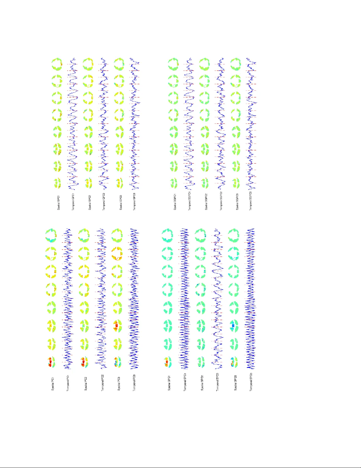
A Generalized Least Squares Matrix Decomp osition Genev era I. Allen ∗ Departmen t of P ediatrics-Neurology , Ba ylor College of Medicine, Jan and Dan Duncan Neurological Research Institute, T exas Children’s Hospital, & Departments of Statistics and Electrical and Computer Engineering, Rice Universit y . Logan Grosenic k Cen ter for Mind, Brain and Computation, Stanford Universit y . Jonathan T a ylor Departmen t of Statistics, Stanford Universit y . August 14, 2018 Abstract V ariables in many massiv e high-dimensional data sets are structured, arising for example from measuremen ts on a regular grid as in imaging and time series or from spatial-temp oral measuremen ts as in climate studies. Classical multiv ariate techniques ignore these structural relationships often resulting in po or performance. W e prop ose a generalization of the singular v alue decomposition (SVD) and principal comp onen ts analysis (PCA) that is appropriate for massiv e data sets with structured v ariables or kno wn tw o-w a y dep endencies. By ﬁnding the b est low rank approximation of the data with respect to a transp osable quadratic norm, our decomposition, entitled the Gen- er alize d le ast squar es Matrix De c omp osition (GMD), directly accoun ts for structural relationships. As many v ariables in high-dimensional settings are often irrelev an t or noisy , we also regularize our matrix decomp osition by adding t wo-w a y penalties to en- courage sparsity or smoothness. W e develop fast computational algorithms using our metho ds to perform generalized PCA (GPCA), sparse GPCA, and functional GPCA on massive data sets. Through simulations and a whole brain functional MRI example w e demonstrate the utilit y of our methodology for dimension reduction, signal recov ery , and feature selection with high-dimensional structured data. Keyw ords : matrix decomposition, singular v alue decomp osition, principal comp o- nen ts analysis, sparse PCA, functional PCA, structured data, neuroimaging. 1 In tro duction Principal comp onen ts analysis (PCA), and the singular v alue decomp osition (SVD) upon whic h it is based, form the foundation of muc h of classical multiv ariate analysis. It is well kno wn, ho wev er, that with both high-dimensional data and functional data, traditional PCA can p erform p o orly (Silverman, 1996; Jolliﬀe et al., 2003; Johnstone and Lu, 2004). Metho ds enforcing sparsity or smo othness on the matrix factors, suc h as sparse or functional PCA, ha v e been shown to consistently recov er the factors in these settings (Silv erman, 1996; Johnstone and Lu, 2004). Recently , these techniques hav e b een extended to regularize b oth ∗ T o whom correspondence should b e addressed. 1 the row and column factors of a matrix (Huang et al., 2009; Witten et al., 2009; Lee et al., 2010). All of these methods, how ev er, can fail to capture relev an t aspects of structured high- dimensional data. In this pap er, we prop ose a general and ﬂexible framework for PCA that can directly account for structural dep endencies and incorp orate tw o-w a y regularization for exploratory analysis of massive structured data sets. Examples of high-dimensional structured data in w hic h classical PCA p erforms p oorly ab ound in areas of biomedical imaging, environmen tal studies, time series and longitudinal studies, and netw ork data. Consider, for example, functional MRIs (fMRIs) which measure three-dimensional images of the brain o ver time with high spatial resolution. Eac h three- dimensional pixel, or v o xel, in the image corresp onds to a measure of the b old oxygenation lev el dep endent (BOLD) resp onse (hereafter referred to as “activ ation”), an indirect measure of neuronal activity at a particular location in the brain. Often these vo xels are vectorized at each time p oin t to form a high-dimensional matrix of vo xels ( ≈ 10,000 - 100,000) by time p oin ts ( ≈ 100 - 10,000) to be analyzed by m ultiv ariate methods. Th us, this data exhibits strong spatial dependencies among the rows and strong temp oral dependencies among the columns (Lindquist, 2008; Lazar, 2008). Multiv ariate analysis tec hniques are often applied to fMRI data to ﬁnd regions of interest, or spatially contiguous groups of v oxels exhibiting strong co-activ ation as well as the time courses asso ciated with these regions of activit y (Lindquist, 2008). Principal components analysis and the SVD, ho w ev er, are rarely used for this purp ose. Man y hav e noted that the ﬁrst several principal comp onen ts of fMRI data app ear to capture spatial and temp oral dep endencies in the noise rather than the patterns of brain activ ation in which neuroscien tists are interested. F urthermore, subsequen t principal comp onen ts often exhibit a mixture of noise dep endencies and brain activ ation suc h that the signal in the data remains unclear (F riston et al., 1999; Calhoun et al., 2001; Thirion and F augeras, 2003; Viviani et al., 2005). This b eha vior of classical PCA is typical when it is applied to structured data with lo w signal compared to the noise dependencies induced b y the data structure. T o understand the p oor performance of the SVD and PCA is these settings, we ex- amine the mo del mathematically . W e observe data Y ∈ < n × p , for which standard PCA considers the following mo del: Y = M + U D V T + E , where M denotes a mean matrix, D the singular v alues, U and V the left and right factors, resp ectiv ely , and E the noise matrix. Implicitly , SVD models assume that the elements of E are indep endently and iden tically distributed, as the SVD is calculated by minimizing the F rob enius norm loss function: || X − U D V T || 2 F = P n i =1 P p j =1 ( X ij − u i D v T j ) 2 , where u i is the i th column of U and v j is analogous and X denotes the centered data, X = Y − M . This sums of squares loss function weigh ts errors asso ciated with each matrix element equally and cross-pro duct errors, b et ween elements X ij and X i 0 j 0 , for example, are ignored. It comes as no surprise then that the F rob enius norm loss and thus the SVD p erform p oorly with data exhibiting strong structural dep endencies among the matrix elemen ts. T o permit un- equal weigh ting of the matrix errors according to the data structure, we assume that the noise is structured: vec( E ) ∼ ( 0 , R − 1 ⊗ Q − 1 ), or the cov ariance of the noise is separable and has a Kronec ker product co v ariance (Gupta and Nagar, 1999). Our loss function, then c hanges from the F rob enius norm to a transp osable quadratic norm that p ermits unequal weigh ting of the matrix error terms based on Q and R : || X − U D V T || 2 Q , R = P n i =1 P p j =1 P n i 0 =1 P p j 0 =1 Q ii 0 R j j 0 ( X ij − u i D v T j )( X i 0 j 0 − u i 0 D v T j 0 ). By ﬁnding the b est lo w rank approximation of the data with resp ect to this transp osable quadratic norm, w e dev elop a decomp osition that directly accounts for tw o-w a y structural dep endencies in the data. This gives us a metho d, Gener alize d PCA , that extends PCA for applications to structured data. While this pap er w as initially under review, previous work on unequal weigh ting of ma- trix elemen ts in PCA via a ro w and column generalizing op erators came to our attention 2 (Escouﬁer, 1977). This so called, “duality approach to PCA” is known in the F rench mul- tiv ariate communit y , but has p erhaps not gained the popularity in the statistics literature that it deserves. Dev eloped predominately in the 1970’s and 80’s for applications in eco- logical statistics, few texts on this were published in English (Escouﬁer, 1977; T enenhaus and Y oung, 1985; Escouﬁer, 1987). Recently , a few w orks review these metho ds in relation to classical multiv ariate statistics (Escouﬁer, 2006; Purdom, 2007; Dra y and Dufour, 2007; Holmes, 2008). While these w orks propose a mathematical framew ork for unequal w eighting matrices in PCA, m uc h more statistical and computational developmen t is needed in order to directly apply these methods to high-dimensional structured data. In this paper, we aim to develop a ﬂexible mathematical framework for PCA that ac- coun ts for known structure and incorp orates regularization in a manner that is computation- ally feasible for analysis of massiv e structured data sets. Our sp eciﬁc contributions include (1) a matrix decomp osition that accounts for known tw o-w a y structure, (2) a framework for tw o-w a y regularization in PCA and in Generalized PCA, and (3) results and algorithms allo wing one to compute (1) and (2) for ultra high-dimensional data. Sp eciﬁcally , b ey ond the previous w ork in this area review ed by Holmes (2008), w e pro vide results allo wing for (i) general weigh ting matrices, (ii) computational approaches for high-dimensional data, and (iii) a framework for tw o-w a y regularization in the con text of Generalized PCA. As our metho ds are ﬂexible and general, they will enjoy wide applicability to a v ariet y of struc- tured data sets common in medical imaging, remote sensing, engineering, environmetrics, and netw orking. The pap er is organized as follows. In Sections 2.1 through 2.5, we dev elop the math- ematical framew ork for our Gener alize d L e ast Squar es Matrix De c omp osition and resulting Generalized PCA. In these sections, we assume that the weigh ting matrices, or quadr atic op er ators are ﬁxed and known. Then, by discussing interp retations of our approac h and relations to existing metho dology , we presen t classes of quadratic op erators in Section 2.6 that are appropriate for many structured data sets. As the fo cus of this pap er is the statis- tical metho dology for PCA with high-dimensional structured data, our inten t here is to give the reader intuition on the quadratic operators and leav e other aspects for future w ork. In Section 3, we prop ose a general framew ork for incorporating t wo-w a y regularization in PCA and Generalized PCA. W e demonstrate ho w this framew ork leads to methods for Sparse and F unctional Generalized PCA. In Section 4, we give results on b oth simulated data and real functional MRI data. W e conclude, in Section 5, with a discussion of the assumptions, implications, and possible extensions of our w ork. 2 A Generalized Least Squares Matrix Decomp osition W e present a generalization of the singular v alue decomp osition (SVD) that incorp orates kno wn dep endencies or structural information ab out the data. Our metho ds can b e used to p erform Generalized PCA for massive structured data sets. 2.1 GMD Problem Here and for the remainder of the pap er, we will assume that the data, X has previously b een centered. W e b egin by reviewing the SVD which can b e written as X = U D V T with the data X ∈ < n × p , and where U ∈ < n × p and V ∈ < p × p are orthonormal and D ∈ < p × p is diagonal with non-negative diagonal elements. Supp ose one wishes to ﬁnd the b est low rank, K < min( n, p ), approximation to the data. Recall that the SVD giv es the best rank- K 3 appro ximation with respect to the F rob enius norm (Ec k art and Y oung, 1936): minimize U :rank( U )= K, D : D ∈D , V :rank( V )= K || X − U D V T || 2 F sub ject to U T U = I ( K ) , V T V = I ( K ) & diag( D ) ≥ 0 . (1) Here, D is the class of diagonal matrices. The solution is given by the ﬁrst K singular v ectors and singular v alues of X . The F rob enius norm weigh ts all errors equally in the loss function. W e seek a general- ization of the SVD that allows for unequal w eigh ting of the errors to accoun t for structure or kno wn dep endencies in the data. T o this end, we introduce a loss function giv en by a transp osable quadratic norm, the Q , R -norm, deﬁned as follo ws: Deﬁnition 1 L et Q ∈ < n × n and R ∈ < p × p b e p ositive semi-deﬁnite matric es, Q , R  0 . Then the Q , R -norm (or semi-norm) is deﬁne d as || X || Q , R = q tr( Q X R X T ) . W e note that if Q and R are b oth p ositive deﬁnite, Q , R  0, then the Q , R -norm is a prop er matrix norm. If Q or R are positive semi-deﬁnite, then it is a semi-norm, meaning that for X 6 = 0, || X || Q , R = 0 if X ∈ nul l ( Q ) or if X T ∈ null ( R ). W e call the Q , R -norm a transp osable quadratic norm, as it right and left m ultiplies X and is th us an extension of the quadratic norm, or “norm induced by an inner pro duct space” (Boyd and V anden b erghe, 2004; Horn and Johnson, 1985). Note that || X || Q , || X || Q , I and || X T || R , || X T || R , I are then quadratic norms. The GMD is then taken to be the b est rank- K approximation to the data with resp ect to the Q , R -norm: minimize U :rank( U )= K, D : D ∈D , V :rank( V )= K || X − U D V T || 2 Q , R sub ject to U T Q U = I ( K ) , V T R V = I ( K ) & diag( D ) ≥ 0 . (2) So we do not confuse the elements of the GMD with that of the SVD, we call U and V the left and right GMD factors resp ectively , and the diagonal elements of D , the GMD v alues. The matrices Q and R are called the left and righ t quadratic op erators of the GMD resp ectiv ely . Notice that the left and right GMD factors are constrained to be orthogonal in the inner pro duct space induced by the Q -norm and R -norm resp ectiv ely . Since the F rob enius norm is a special case of the Q , R -norm, the GMD is in fact a generalization of the SVD. W e pause to motiv ate the rationale for ﬁnding a matrix decomp osition with respect to the Q , R -norm. Consider a matrix-v ariate Gaussian matrix, X ∼ N n,p ( U D V T , Q − 1 , R − 1 ), or vec( X ) ∼ N (v ec( U D V T ) , R − 1 ⊗ Q − 1 ) in terms of the familiar m ultiv ariate normal. The normal log-likelihoo d can be written as: ` ( X | Q − 1 , R − 1 ) ∝ tr  Q ( X − U D V T ) R ( X − U D V T ) T  = || X − U D V T || 2 Q , R . Th us, as the F rob enius norm loss of the SVD is prop ortional to the log-likelihoo d of the spherical Gaussian with mean U D V T , the Q , R -norm loss is proportional to the log- lik eliho od of the matrix-v ariate Gaussian with mean U D V T , row cov ariance Q − 1 , and column co v ariance R − 1 . In general, using the Q , R -norm loss assumes that the co v ariance of the data arises from the Kroneck er pro duct b et w een the row and column co v ariances, or that the co v ariance structure is separable. Several statistical tests exist to chec k these assumptions with real data (Mitc hell et al., 2006; Li et al., 2008). Hence, if the dep endence structure of the data is known, taking the quadratic operators to b e the in v erse cov ariance or precision matrices directly accounts for t w o-wa y dep endencies in the data. W e assume that Q and R are kno wn in the dev elopment of the GMD and discuss p ossible choices for these with structured data in Section 2.5. 4 2.2 GMD Solution The GMD solution, ˆ X = U ∗ D ∗ ( V ∗ ) T , is comprised of U ∗ , D ∗ and V ∗ , the optimal points minimizing the GMD problem (2). The following result states that the GMD solution is an SVD of an altered data matrix. Theorem 1 Supp ose rank( Q ) = l and rank( R ) = m . De c omp ose Q and R by letting Q = ˜ Q ˜ Q T and R = ˜ R ˜ R T wher e ˜ Q ∈ < n × l and ˜ R ∈ < p × m ar e of ful l c olumn r ank. Deﬁne ˜ X = ˜ Q T X ˜ R and let ˜ X = ˜ U ˜ D ˜ V T b e the SVD of ˜ X . Then, the GMD solution, ˆ X = U ∗ D ∗ ( V ∗ ) T , is given by the GMD factors U ∗ = ˜ Q − 1 ˜ U and V ∗ = ˜ R − 1 ˜ V and the GMD values, D ∗ = ˜ D . Her e, ˜ Q − 1 and ˜ R − 1 ar e any left matrix inverse: ( ˜ Q − 1 ) T ˜ Q = I ( l ) and ( ˜ R − 1 ) T ˜ R = I ( m ) . W e make som e brief commen ts regarding this result. First, the decomposition, Q = ˜ Q ˜ Q T where ˜ Q ∈ < n × l is of full column rank, exists since Q  0 (Horn and Johnson, 1985); the decomp osition for R exists similarly . A p ossible form of this decomp osition, the resulting ˜ X , and the GMD solution ˆ X can b e obtained from the eigen v alue decomp osition of Q and R : Q = Γ Q Λ Q Γ T Q and R = Γ R Λ R Γ T R . If Q is full rank, then w e can tak e ˜ Q = Q 1 / 2 = Γ Q Λ 1 / 2 Q Γ T Q , giving the GMD factor U ∗ = Γ Q Λ − 1 / 2 Q Γ T Q ˜ U , and similarly for R and V . On the other hand, if Q  0, then a p ossible v alue for ˜ Q is Γ Q ( · , 1 : l ) Λ 1 / 2 Q (1 : l , 1 : l ), giving an n × l matrix with full column rank. The GMD factor, U ∗ is then given b y Γ Q ( · , 1 : l ) Λ − 1 / 2 Q (1 : l, 1 : l ) ˜ U . F rom Theorem 1, w e see that the GMD solution can b e obtained from the SVD of ˜ X . Let us assume for a moment that X is matrix-v ariate Gaussian with ro w and column co v ariance Q − 1 and R − 1 resp ectiv ely . Then, the GMD is lik e taking the SVD of the spher e d data, as right and left multiplying by ˜ Q and ˜ R yields data with identit y cov ariance. In other words, the GMD de-correlates the data so that the SVD with equally w eighted errors is appropriate. While the GMD v alues are the singular v alues of this sphered data, the cov ariance is multiplied back into the GMD factors. This relationship to the matrix-v ariate normal also b egs the question, if one has data with ro w and column correlations, wh y not take the SVD of the tw o-w ay sphered or “whitened” data? This is inadvisable for several reasons. First, pre-whitening the data and then taking the SVD yields matrix factors that are in the wrong basis and are thus unin terpretable in the original data space. Given this, one may adv ocate pre-whitening, taking the SVD and then re-whitening, or in other words multiplying the correlation back in to the SVD factors. This approach, how ev er, is still problematic. In the sp ecial case where Q and R are of full rank, the GMD solution is exactly to same as this pre and re-whitening approac h. In the general case where Q and R are p ositive semi-deﬁnite, how ev er, whitening cannot b e directly performed as the co v ariances are not full rank. In the following section, we will sho w that the GMD solution can be computed without taking an y matrix inv erses, square ro ots or eigendecompositions and is th us computationally more attractive than naive whitening. Finally , as our even tual goal is to develop a framework for b oth structured data and tw o- w ay regularization, naive pre-whitening and then re-whitening of the data would destroy an y estimated sparsity or smo othness from regularization methods and is thus undesirable. Therefore, the GMD solution given in Theorem 1 is the mathematically correct wa y to “whiten” the data in the context of the SVD and is sup erior to a naive whitening approach. Next, w e explore some of the mathematical properties of our GMD solution, ˆ X = U ∗ D ∗ ( V ∗ ) T in the follo wing corollaries: Corollary 1 The GMD solution is the glob al minimizer of the GMD pr oblem, (2) . 5 Corollary 2 Assume that r ang e ( Q ) ∩ nul l ( X ) = ∅ and r ang e ( R ) ∩ nul l ( X ) = ∅ . Then, ther e exists at most k = min { rank( X ) , rank( Q ) , rank( R ) } non-zer o GMD values and c orr e- sp onding left and right GMD factors. Corollary 3 With the assumptions and k deﬁne d as in Cor ol lary 2, the r ank- k GMD solution has zer o r e c onstruction err or in the Q , R -norm. If in addition, k = rank( X ) and Q and R ar e ful l r ank, then X ≡ U ∗ D ∗ ( V ∗ ) T , that is, the GMD is an exact matrix de c omp osition. Corollary 4 The GMD values, D ∗ , ar e unique up to multiplicity. If in addition, Q and R ar e ful l r ank and the non-zer o GMD values ar e distinct, then the GMD factors U ∗ and V ∗ c orr esp onding to the non-zer o GMD values ar e essential ly unique (up to a sign change) and the GMD factorization is unique. Some further comments on these results are w arranted. In particular, Theorem 1 is straigh tforward and less interesting when Q and R are full rank, the case discussed in (Escouﬁer, 2006; Purdom, 2007; Holmes, 2008). When the quadratic op erators are positive semi-deﬁnite, how ev er, the fact that a global minimizer to the GMD problem, which is non-con vex, that has a closed form can b e obtained is not immediately clear. The result stems from the relation of the GMD to the SVD and the fact that the latter is a unique matrix decomposition in a lo w er dimensional subspace deﬁned in Corollary 2. Also note that when Q and R are full rank the GMD is an exact matrix decomp osition; in the alternativ e scenario, w e do not reco v er X exactly , but obtain zero reconstruction error in the Q , R -norm. Finally , we note that when Q and R are rank deﬁcient, there are p ossibly many optimal p oin ts for the GMD factors, although the resulting GMD solution is still a global minimizer of the GMD problem. In Section 2.6, w e will see that p ermitting the quadratic op erators to b e positive semi-deﬁnite allows for muc h greater ﬂexibility when mo deling high-dimensional structured data. 2.3 GMD Algorithm While the GMD solution giv en in Theorem 1 is conceptually simple, its computation, based on computing ˜ Q , ˜ R and the SVD of ˜ X , is infeasible for massiv e data sets common in neuroimaging. W e seek a metho d of obtaining the GMD solution that a v oids computing and storing ˜ Q and ˜ R and thus p ermits our metho ds to b e used with massive structured data sets. Prop osition 1 If ˆ u and ˆ v ar e initialize d such that ˆ u T Q u ∗ 6 = 0 and ˆ v T Q v ∗ 6 = 0 , then A lgorithm 1 c onver ges to the GMD solution given in The or em 1, the glob al minimizer of the GMD pr oblem. If in addition, Q and R ar e ful l r ank, then it c onver ges to the unique glob al solution. In Algorithm 1, w e giv e a metho d of computing the comp onen ts of the GMD solu- tion that is a v ariation of the familiar p o wer method for calculating the SVD (Golub and V an Loan, 1996). Prop osition 1 states that the GMD Algorithm based on this p ow er metho d con verges to the GMD solution. Notice that we do not need to calculate ˜ Q and ˜ R and thus, this algorithm is less computationally in tensive for high-dimensional data sets than ﬁnding the solution via Theorem 1 or the computational approac hes given in Escouﬁer (1987) for p ositiv e deﬁnite operators. A t this point, w e pause to discuss the name of our matrix decomposition. Recall that the p o w er metho d, or alternating least squares method, sequen tially estimates u with v ﬁxed and vice versa by solving least squares problems and then re-scaling the estimates. Eac h 6 Algorithm 1 GMD Algorithm (P o w er Metho d) 1. Let ˆ X (1) = X and initialize u 1 and v 1 . 2. F or k = 1 . . . K : (a) Rep eat un til conv ergence: • Set u k = ˆ X ( k ) R v k || ˆ X ( k ) R v k || Q . • Set v k = ( ˆ X ( k ) ) T Q u k || ( ˆ X ( k ) ) T Q u k || R . (b) Set d k = u T k Q ˆ X ( k ) R v k . (c) Set ˆ X ( k +1) = ˆ X ( k ) − u k d k v T k . 3. Return U ∗ = [ u 1 , . . . , u K ], V ∗ = [ v 1 , . . . v K ] and D ∗ = diag( d 1 , . . . d K ). step of the GMD algorithm, then, estimates the factors by solving the follo wing generalized least squares problems and re-scaling: || X − ( d 0 u 0 ) v T || 2 Q and || X T − ( d 0 v 0 ) u T || 2 R . This is then the inspiration for the name of our matrix decomposition. 2.4 Generalized Principal Comp onen ts In this section w e show that the GMD can b e used to p erform Generalized Principal Com- p onen ts Analysis (GPCA). Note that this result was ﬁrst sho wn in Escouﬁer (1977) for p ositiv e deﬁnite generalizing operators, but we review it here for completeness. The results in the previous section allo w one to compute these GPCs for high-dimensional data when the quadratic operators may not b e full rank and w e wish to a void computing SVDs and eigen v alue decomp ositions. Recall that the SVD problem can b e written as ﬁnding the linear combination of v ariables maximizing the sample v ariance such that these linear combinations are orthonormal. F or GPCA, w e seek to pro ject the data onto the linear combination of v ariables such that the sample v ariance is maximized in a space that accoun ts for the structure or dep endencies in the data. By transforming all inner product spaces to those induced by the Q , R -norm, we arriv e at the following Generalized PCA problem: maximize v k v T k R X T Q X R v k sub ject to v T k R v k = 1 & v T k R v k 0 = 0 ∀ k 0 < k. (3) Notice that the loadings of the GPCs are orthogonal in the R -norm. The k th GPC is then giv en by z k = X R v k . Prop osition 2 The solution to the k th Gener alize d princip al c omp onent pr oblem, (3) , is given by the k th right GMD factor. Corollary 5 The pr op ortion of varianc e explaine d by the k th Gener alize d princip al c omp o- nent is given by d 2 k / || X || 2 Q , R . Just as the SVD can b e used to ﬁnd the principal comp onen ts, the GMD can b e used to ﬁnd the generalize d principal comp onen ts. Hence, GPCA can b e p erformed using the GMD algorithm which do es not require calculating ˜ Q and ˜ R . This allo ws one to eﬃciently p erform GPCA for massiv e structured data sets. 7 2.5 In terpretations, Connections & Quadratic Op erators In the previous sections, w e ha ve introduced the metho dology for the Generalized Least Squares Matrix Decomp osition and ha v e outlined how this can be used to compute GPCs for high-dimensional data. Here, we pause to discuss some interpretations of our methods and ho w they relate to existing metho dology for non-linear dimension reduction. These in terpretations and relationships will help us understand the role of the quadratic op erators and the classes of quadratic op erators that may b e appropriate for types of structured high- dimensional data. As the fo cus of this pap er is the statistical metho dology of PCA for high-dimensional structured data, w e leav e m uch of the study of quadratic op erators for sp eciﬁc applications as future work. First, there are many connections and in terpretations of the GMD in the realm of clas sical matrix analysis and m ultiv ariate analysis. W e will refrain from listing all of these here, but note that there are close relations to the GSVD of V an Loan (1976) and generalized eigen v alue problems (Golub and V an Loan, 1996) as well as statistical metho ds such as discriminan t analysis, canonical correlations analysis, and corresp ondence analysis. Many of these connections are discussed in Holmes (2008) and Purdom (2007). Recall also that the GMD can b e interpreted as a maximum likelihoo d problem for the matrix-v ariate normal with ro w and column inv erse cov ariances ﬁxed and known. This connection yields tw o in terpretations worth noting. First, the GMD is an extension of the SVD to allow for heteroscedastic (and separable) ro w and column errors. Thus, the quadratic operators act as weigh ts in the matrix decomposition to p ermit non i.i.d. errors. The second relationship is to whitening the data with kno wn ro w and column cov ariances prior to dimension reduction. As discussed in Section 2.2, our metho dology oﬀers the prop er mathematical context for this whitening with many adv antages ov er a naiv e whitening approach. Next, the GMD can b e in terpreted as decomp osing a co v ariance op erator. Let us assume that the data follows a simple model: X = S + E , where S = P K k =1 φ k u k v T k with the factors v k and u k ﬁxed but unknown and with the amplitude φ k random, and E ∼ N n,p (0 , Q − 1 , R − 1 ). Then the (v ectorized) cov ariance of the data can b e written as: Co v(vec( X )) = K X k =1 V ar( φ k ) v k v T k ⊗ u k u T k + R − 1 ⊗ Q − 1 , suc h that V T R V = I and U T Q U = I . In other words, the GMD decomp oses the co v ari- ance of the data in to a signal comp onen t and a noise comp onent such that the eigenv ectors of the signal comp onen t are orthonormal to those of the noise comp onen t. This is an imp or- tan t interpretation to consider when selecting quadratic operators for particular structured data sets, discussed subsequently . Finally , there is a close connection b et ween the GMD and smoothing dimension reduction metho ds. Notice that from Theorem 1, the GMD factors U and V will b e as smo oth as as the smallest eigenv ectors corresp onding to non-zero eigen v alues of Q and R resp ectiv ely . Th us, if Q and R are taken as smo othing op erators, then the G MD can yield smo othed factors. Giv en these interpretations of the the GMD, w e consider classes of quadratic operators that may b e appropriate when applying our methods to structured data: 1. Mo del-based and parametric op erators. The quadratic operators could b e taken as the in verse co v ariance matrices implied by common mo dels employ ed with structured data. These include well-kno wn time series autoregressive and moving av erage pro cesses, random ﬁeld models used for spatial data, and Gaussian Marko v random ﬁelds. 2. Graphical op erators. As many types of structured data can b e w ell represen ted b y a graphical mo del, the graph Laplacian op erator, deﬁned as the diﬀerence b etw een 8 the degree and adjacency matrix, can b e used as a quadratic operator. Consider, for example, image data sampled on a regular mesh grid; a lattice graph connecting all the nearest neigh bors w ell represents the structure of this data. 3. Smo othing / Structural embedding op erators. T aking quadratic op erators as smo oth- ing matrices common in functional data analysis will yield smo othed GMD factors. In these smo othing matrices, tw o v ariables are t ypically weigh ted inv ersely prop ortional to the distance b et w een them. Thus, these can also b e thought of as structural em- b edding matrices, increasing the weigh ts in the loss function b et w een v ariables that are close together on the structural manifold. While this list of p oten tial classes of quadratic op erators is most certainly incomplete, these provide the ﬂexibility to mo del many types of high-dimensional structured data. No- tice that many examples of quadratic op erators in each of these classes are closely related. Consider, for example, regularly spaced ordered v ariables as often seen in time series. A graph Laplacian of a nearest neighbor graph is tri-diagonal, is nearly equiv alen t except for b oundary p oin ts to the squared second diﬀerences matrix often used for in v erse smoothing in functional data analysis (Ramsa y, 2006), and has the same zero pattern as the inv erse co v ariance of an autoregressive and mo ving av erage order one pro cess (Shaman, 1969; Gal- braith and Galbraith, 1974). Additionally , the zero patterns in the in v erse cov ariance matrix of Gaussian Mark o v random ﬁelds are closely connected to Mark ov netw orks and undirected graph Laplacians (Rue and Held, 2005). A recent pap er, Lindgren et al. (2011), shows how common stationary random ﬁeld mo dels speciﬁed by their co v ariance function suc h as the Mat ´ ern class can be derived from functions of a graph Laplacian. Finally , notice that graph- ical op erators such as Laplacians and smo othing matrices are typically not p ositiv e deﬁnite. Th us, our framework allowing for general quadratic op erators in Section 2.2 op ens more p ossibilities than diagonal w eigh ting matrices (Dra y and Dufour, 2007) and those used in ecological applications (Escouﬁer, 1977; T enenhaus and Y oung, 1985). There are many further connections of the GMD when employ ed with sp eciﬁc quadratic op erators b elonging to the ab o ve classes and other recent metho ds for non-linear dimension reduction. Let us ﬁrst consider the relationship of the GMD to F unctional PCA (FPCA) and the more recent tw o-w ay FPCA. Silv erman (1996) ﬁrst sho w ed that for discretized functional data, FPCA can b e obtained by half-smo othing; Huang et al. (2009) elegantly extended this to tw o-w a y half-smo othing. Let us consider the latter where ro w and column smo othing matrices, S u = ( I + λ u Ω u ) − 1 and S v = ( I + λ v Ω v ) − 1 resp ectiv ely , are formed with Ω b eing a p enalty matrix suc h as to giv e the squared second diﬀerences for example (Ramsa y, 2006) related to the structure of the row and column v ariables. Then, Huang et al. (2009) show ed that t wo-w a y FPCA can b e p erformed b y t wo-w a y half smo othing: (1) take the SVD of X 0 = S 1 / 2 u X S 1 / 2 v , then (2) the FPCA factors are U = S 1 / 2 u U 0 and V = S 1 / 2 v V 0 . In other w ords, a half smoother is applied to the data, the SVD is taken and another half-smo other is applied to the SVD factors. This pro cedure is quite similar to the GMD solution outlined in Theorem 1. Let us assume that Q and R are smoothing matrices. Then, our GMD solution is essentially lik e half-smo othing the data, taking the SVD then in verse half-smoothing the SVD factors. Th us, unlike tw o-w a y FPCA, the GMD does not half-smo oth both the data and the factors, but only the data and then ﬁnds factors that are in con trast to the smoothed data. If the con v erse is true and w e take Q and R to be “inv erse smo others” suc h as a graph Laplacian, then this in v erse smo other is applied to the data, the SVD is taken and the resulting factors are smoothed. Dissimilar to tw o-w a y FPCA whic h p erforms tw o smoothing op erations, the GMD essentially applies one smoothing op eration and one in v erse smo othing op eration. The GMD also shares similarities to other non-linear dimension reduction techniques suc h as Sp ectral Clustering, Lo cal Linear Embedding, Manifold Learning, and Lo cal Multi- 9 Dimensional Scaling. Spectral clustering, Laplacian em b edding, and manifold learning all inv olv e taking an eigendecomp osition of a Laplacian matrix, L , capturing the dis- tances or relationships b et w een v ariables. The eigen vectors corresp onding to the smallest eigen v alues are of interest as these corresp ond to minimizing a weigh ted sums of squares: f T L f = P i P i 0 L i,i 0 ( f i − f i 0 ) 2 , ensuring that the distances betw een neighboring v ariables in the reconstruction f are small. Supp ose Q = L and R = I , then the GMD minimizes: P i P i 0 L i,i 0 ( X i − u i D V T ) 2 , similar to the Laplacian embedding criterion. Thus, the GMD with quadratic op erators related to the structure or distance b etw een v ariables ensures that the errors b etw een the data and its low rank approximation are smallest for those v ariables that are close in the data structure. This concept is also closely related to Lo cal Multi- Dimensional Scaling which w eights MDS lo cally by placing more weigh t on v ariables that are in close proximit y (Chen and Buja, 2009). The close connections of the GMD to other recent non-linear dimension reduction tec h- niques provides additional con text for the role of the quadratic op erators. Sp eciﬁcally , these examples indicate that for structured data, it is often not necessary to directly estimate the quadratic op erators from the data. If the quadratic op erators are tak en as smo othing matrices, structural embedding matrices or Laplacians related to the distances betw een v ari- ables, then the GMD has similar prop erties to many other non-linear unsup ervised learning metho ds. In summary , when v arious quadratic op erators that enco de data structure such as the distances b etw een v ariables are employ ed, the GMD can b e in terpreted as (1) ﬁnding the basis vectors of the co v ariance that are separate (and orthogonal) to that of the data structure, (2) ﬁnding factors that are smo oth with resp ect to the data structure, or (3) ﬁnding an appro ximation to the data that has small reconstruction error with resp ect to the structural manifold. Through simulations in Section 4.1, we will explore the p erformance of the GMD for diﬀerent combinations of graphical and smo othing op erators enco ding the kno wn data structure. As there are many examples of structured high-dimensional data (e.g. imaging, neuroimaging, microscopy , h yp erspectral imaging, c hemometrics, remote sensing, en vironmental data, sensor data, and net work data), these classes of quadratic op erators pro vide a wide range of p oten tial applications for our metho dology . 3 Generalized P enalized Matrix F actorization With high-dimensional data, many hav e advocated regularizing principal comp onen ts by either automatically selecting relev an t features as with Sparse PCA or by smo othing the factors as with F unctional PCA (Silv erman, 1996; Jolliﬀe et al., 2003; Zou et al., 2006; Shen and Huang, 2008; Huang et al., 2009; Witten et al., 2009; Lee et al., 2010). Regularized PCA can b e imp ortan t for massive structured data as well. Consider spatio-temp oral fMRI data, for example, where man y spatial locations or vo xels in the brain are inactiv e and the time courses are often extremely noisy . Automatic feature selection of relev an t v o xels and smo othing of the time series in the context of PCA for structured data would thus b e an imp ortan t contribution. In this section, we seek a framew ork for regularizing the factors of the GMD by placing penalties on each factor. In developing this framew ork, we rev eal an imp ortan t result demonstrating the general class of p enalties that can b e placed on matrix factors that are to be estimated via deﬂation: the penalties m ust b e norms or semi-norms. 3.1 GPMF Problem Recen tly , man y hav e suggested regularizing the factors of the SVD by forming tw o-w a y p enalized regression problems (Huang et al., 2009; Witten et al., 2009; Lee et al., 2010). W e brieﬂy review these existing approac hes to understand ho w to frame a problem that allo ws us to place general sparse or smo oth p enalties on the GMD factors. 10 W e compare the optimization problems of these three approaches for computing a single- factor tw o-w a y regularized matrix factorization: Witten et al. (2009) : maximize v , u u T X v sub ject to u T u ≤ 1 , v T v ≤ 1 , P 1 ( u ) ≤ c 1 , & P 2 ( v ) ≤ c 2 . Huang et al. (2009) : maximize v , u u T X v − λ 2 P 1 ( u ) P 2 ( v ) . Lee et al. (2010) : maximize v , u u T X v − 1 2 u T u v T v − λ u 2 P 1 ( u ) − λ v 2 P 2 ( v ) . Here, c 1 and c 2 are constants, P 1 () and P 2 () are p enalt y functions, and λ , λ v and λ u are p enalt y parameters. These optimization problems are attractive as they are bi-concav e in u and v , meaning that they are concav e in u with v ﬁxed and vice versa. Th us, a simple maximization strategy of iteratively maximizing with resp ect to u and v results in a monotonic ascent algorithm con v erging to a lo cal maxim um. These metho ds, how ev er, diﬀer in the t yp es of p enalties that can b e emplo yed and their scaling of the matrix factors. Witten et al. (2009) explicitly restrict the norms of the factors, while the constraints in the metho d of Huang et al. (2009) are implicit b ecause of the t yp es of functional data p enalties employ ed. Thus, for these metho ds, as the constan ts c 1 and c 2 or the p enalt y parameter, λ approac h zero, the SVD is returned. This is not the case, how ev er, for problem in Lee et al. (2010) where the factors are not constrained in the optimization problem, although they are later scaled in their algorithm. Also, restricting the scale of the factors a voids possible numerical instabilities when employing the iterative estimation algorithm (see esp ecially the supplemen tary materials of Huang et al. (2009)). Th us, we prefer the former t w o approac hes for these reasons. In Witten et al. (2009), how ev er, only the lasso and fused lasso p enalt y functions are emplo yed and it is unclear whether other p enalties may b e used in their framew ork. Huang et al. (2009), on the other hand, limit their consideration to quadratic functional data p enalties, and their optimization problem do es not implicitly scale the factors for other t yp es of p enalties. As we wish to employ general p enalties, sp eciﬁcally sparse and smo oth p enalties, on the matrix factors, we adopt an optimization problem that leads to simple solutions for the factors with a wide class of penalties, as discussed in the subsequen t section. W e then, deﬁne the single-factor Gener alize d Penalize d Matrix F actorization (GPMF) problem as the follo wing: maximize v , u u T Q X R v − λ v P 1 ( v ) − λ u P 2 ( u ) sub ject to u T Q u ≤ 1 & v T R v ≤ 1 , (4) where, as before, λ v and λ u are penalty parameters and P 1 () and P 2 () are p enalt y functions. Note that if λ u = λ v = 0, then the left and right GMD factors can b e found from (4), as desired. Strictly sp eaking, this problem is the Lagrangian of the problem in tro duced in Witten et al. (2009), k eeping in mind that we should in terpret the inner products as those induced by the Q , R -norm. As w e will see in Theorem 2 in the next section, this problem is tractable for many common choices of p enalt y functions and av oids the scaling problems of other approac hes. 3.2 GPMF Solution W e solve the GPMF criterion, (4), via blo c k co ordinate ascent by alternating maximizing with resp ect to u then v . Note that if λ v = 0 or λ u = 0, then the co ordinate up date for u or v is giv en b y the GMD up dates in Step (b) (i) of the GMD Algorithm. Consider the follo wing result: 11 Theorem 2 Assume that P 1 () and P 2 () ar e c onvex and homo gene ous of or der one: P ( cx ) = cP ( x ) ∀ c > 0 . L et u b e ﬁxe d at u 0 or v b e ﬁxe d at v 0 such that u 0 T Q X 6 = 0 or v 0 T R X T 6 = 0 . Then, the c o or dinate up dates, u ∗ and v ∗ , maximizing the single-factor GPMF pr oblem, (4) , ar e given by the fol lowing: L et ˆ v = argmin v { 1 2 || X T Q u 0 − v || 2 R + λ v P 1 ( v ) } and ˆ u = argmin u { 1 2 || X R v 0 − u || 2 Q + λ u P 2 ( u ) } . Then, v ∗ = ( ˆ v / || ˆ v || R if || ˆ v || R > 0 0 otherwise , & u ∗ = ( ˆ u / || ˆ u || Q if || ˆ u || Q > 0 0 otherwise . Theorem 2 states that for p enalt y functions that are con v ex and homogeneous of order one, the co ordinate up dates giving the single-factor GPMF solution can b e obtained by a generalized p enalized regression problem. Note that p enalt y functions that are norms or semi-norms are necessarily conv ex and homogeneous of order one. This class of functions includes common p enalties such as the lasso (Tibshirani, 1996), group lasso (Y uan and Lin, 2006), fused lasso (Tibshirani et al., 2005), and the generalized lasso (Tibshirani and T aylor, 2011). Imp ortan tly , these do not include the ridge p enalt y , elastic net, concav e p enalties such as SCAD, and quadratic smo othing p enalties commonly used in functional data analysis. Many of the penalized regression solutions for these p enalties, ho w ever, can b e appro ximated by p enalties that are norms or semi-norms. F or instance, to mimic the eﬀect of a giv en quadratic p enalty , one may use the square-ro ot of this quadratic p enalt y . Similarly , the natural ma jorization-minimization algorithms for SCAD-t ype p enalties (F an and Li, 2001a) inv olv e conv ex piecewise linear ma jorizations of the p enalties that satisfy the conditions of Theorem 2. Th us, our single-factor GPMF problem both a v oids the complicated scaling problems of some existing tw o-w a y regularized matrix factorizations, and still permits a wide class of p enalties to be used within our framework. F ollowing the structure of the GMD Algorithm, the multi-factor GPMF can b e computed via the p o w er metho d framew ork. That is, the GPMF algorithm replaces Steps (b) (i) of the GMD Algorithm with the single factor GPMF updates giv en in Theorem 2. This follo ws the same approach as that of other tw o-w ay matrix factorizations (Huang e t al., 2009; Witten et al., 2009; Lee et al., 2010). Notice that unlik e the GMD, subsequent factors computed via this greedy deﬂation approach will not b e orthogonal in the Q , R -norm to previously computed comp onen ts. Man y ha ve noted in the Sparse PCA literature for example, that orthogonality of the sparse components is not necessarily w arran ted (Jolliﬀe et al., 2003; Zou et al., 2006; Shen and Huang, 2008). If only one factor is penalized, ho wev er, orthogonalit y can b e enforced in subsequent components via a Gram-Sc hmidt sc heme (Golub and V an Loan, 1996). In the follo wing sections, we giv e methods for obtaining the single-factor GPMF up dates for sparse or smo oth p enalt y types, noting that man y other p enalties may also b e employ ed with our methods. As the single-factor GPMF problem is symmetric in u and v , we solve the R -norm p enalized regression problem in v , noting that the solutions are analogous for the Q -norm penalized problem in u . 3.3 Sparsit y: Lasso and Related P enalties With high-dimensional data, sparsit y in the factors or principal components yields greater in terpretability and, in some cases ha v e b etter prop erties than un-p enalized principal com- p onen ts (Jolliﬀe et al., 2003; Johnstone and Lu, 2004). With neuroimaging data, sparsity in the factors asso ciated with the vo xels is particularly w arran ted as in most cases relatively few brain regions are exp ected to truly contribute to the signal. Hence, we consider our GPMF problem, (4), with the lasso (Tibshirani, 1996), or ` 1 -norm p enalt y , commonly used to encourage sparsit y . 12 The p enalized regression problem given in Theorem 2 can b e written as a lasso problem: 1 2 || X T Q u − v || 2 R + λ v || v || 1 . If R = I , then the solution for ˆ v is obtained b y simply applying the soft thresholding op erator: ˆ v = S ( X T Q u , λ ), where S ( x, λ ) = sign( x )( | x | − λ ) + (Tibshirani, 1996). When R 6 = I , the solution is not as simple: Claim 1 If R is diagonal with strictly p ositive diagonal entries, then ˆ v minimizing the R -norm lasso pr oblem is given by ˆ v = S ( X T Q u , λ v R − 1 1 ( p ) ) . Claim 2 The solution, ˆ v , that minimizes the R -norm lasso pr oblem c an b e obtaine d by iter ative c o or dinate-desc ent wher e the solution for e ach c o or dinate ˆ v j is given by: ˆ v j = 1 R j j S  R rj X T Q u − R j, 6 = j ˆ v 6 = j , λ v  , with the subscript R rj denoting the r ow elements as- so ciate d with c olumn j of R . Claim 1 states that when R is diagonal, the solution for v can be obtained b y soft thresholding the elements of y by a vector p enalty parameter. F or general R , Claim 2 giv es that we can use co ordinate-descen t to ﬁnd the solution without having to compute ˜ R . Thus, the sparse single-factor GPMF solution can b e calculated in a computationally eﬃcien t manner. One may further improv e the sp eed of co ordinate-descen t b y emplo ying w arm starts and iterating o v er active co ordinates as described in F riedman et al. (2010). W e hav e discussed the details of computing the GPMF factors for the lasso p enalty , and similar techniques can b e used to eﬃcien tly compute the solution for the group lasso (Y uan and Lin, 2006), fused lasso (Tibshirani et al., 2005), generalized lasso (Tibshirani and T aylor, 2011) and other sparse conv ex p enalties. As men tioned, we limit our class of p enalt y functions to those that are norms or semi-norms, which do es not include p opular conca ve p enalties suc h as the SCAD p enalt y (F an and Li, 2001b). As mentioned ab o v e, these p enalties, ho wev er, can still b e used in our framework as concav e p enalized regression problems can b e solv ed via iterativ e w eigh ted lasso problems (Mazumder et al., 2009). Th us, our GPMF framew ork can b e used with a wide range of p enalties to obtain sparsity in the factors. Finally , we note that as our GMD Algorithm can b e used to p erform GPCA, the sparse GPMF framework can b e used to ﬁnd sparse generalized principal components by setting λ u = 0 in (4). This is an approach w ell-studied in the Sparse PCA literature (Shen and Huang, 2008; Witten et al., 2009; Lee et al., 2010). 3.3.1 Smo othness: Ω-norm Penalt y & F unctional Data In addition to sparseness, there is muc h interest in p enalties that encourage smo othness, esp ecially in the con text of functional data analysis. W e sho w how the GPMF can b e used with smo oth p enalties and prop ose a generalized gradient descent metho d to solve for these smo oth GPMF factors. Many ha v e proposed to obtain smo othness in the factors by using a quadratic p enalt y . Rice and Silverman (1991) suggested P ( v ) = v T Ω v , where Ω is the matrix of squared second or fourth diﬀerences. As this p enalty is not homogeneous of order one, we use the Ω -norm p enalt y: P ( v ) = ( v T Ω v ) − 1 / 2 = || v || Ω . Since this p enalty is a norm or a semi-norm, the GPMF solution given in Theorem 2 can b e employ ed. W e see k to minimize the follo wing Ω -norm p enalized regression problem: 1 2 || X T Q u − v || 2 R + λ v || v || Ω . Notice that this problem is similar in structure to the group lasso problem of Y uan and Lin (2006) with one group. T o solve the Ω -norm p enalized regression problem, w e use a generalized gradien t descent metho d. (W e note that there are more elab orate ﬁrst order solvers, introduced in recent w orks suc h as Beck er et al. (2010, 2009), and w e describ e a simple version of such solvers). Supp ose Ω has rank k . Then, set y = X T Q u , and deﬁne B as B =  Ω − 1 / 2 N  where 13 Ω − 1 / 2 ∈ < k × p and N ∈ < ( p − k ) × p . The rows of N are taken to span the null space of Ω , and Ω − 1 / 2 is tak en to satisfy ( Ω − 1 / 2 ) T Ω Ω − 1 / 2 = P Ω , the Euclidean pro jection onto the column space of Ω . The matrices Ω − 1 / 2 and N can b e found from the full eigen v alue decomp osition of Ω , Ω = Γ Λ 2 Γ T . Assuming Λ is in decreasing order, w e can take Ω − 1 / 2 to b e Λ − 1 (1 : k , 1 : k )( Γ (1 : k , · )) T and N to b e the last p − k ro ws of Γ . If Ω is taken to denote the squared diﬀerences, for example, then N can b e tak en as a row of ones. F or the squared second diﬀerences, N can b e set to hav e tw o ro ws: a row of ones and a row with the linear sequence 1 , . . . , p . Ha ving found Ω − 1 / 2 and N , we re-parametrize the problem by taking a non-degenerate linear transformation of v by setting B − 1 v =  w η  so that B w = v . T aking Ω 1 / 2 to b e Λ (1 : k , 1 : k )( Γ (1 : k , · )) T , w e note that k v k Ω = k Ω 1 / 2 v k 2 = k Ω 1 / 2 ( Ω − 1 / 2 w + N η ) k 2 = k w k 2 , as desired. The Ω -norm p enalized regression problem, written in terms of ( w , η ) therefore has the form 1 2 || y − Ω − 1 / 2 w − N η || 2 R + λ v || w || 2 . (5) The solutions of (5) are in one-to-one corresp ondence to those of the Ω -norm regression problem via the relation B w = v and hence, it is suﬃcient to solve (5). Consider the follo wing algorithm and result: Algorithm 2 Algorithm for re-parametrized Ω -norm p enalized regres sion. 1. Let L > 0 be suc h that || B T R B || op < L and initialize w (0) . 2. Deﬁne ˜ w ( t ) = w ( t ) + 1 L B T R  y − Ω − 1 / 2 w ( t ) − N η ( t )  . Set w ( t +1) =  1 − λ v L || ˜ w ( t ) || 2  + ˜ w ( t ) . 3. Set η ( t +1) = ( N T R N ) †  N T R ( y − Ω − 1 / 2 w ( t +1) )  . 4. Rep eat Steps (b)-(c) until conv ergence. Prop osition 3 The v ∗ minimizing the Ω -norm p enalize d r e gr ession pr oblem is given by v ∗ = B  w ∗ η ∗  wher e w ∗ and η ∗ ar e the solutions of Algorithm 2. Since our problem employs a monotonic increasing function of the quadratic smoothing p enalt y , || v || 2 Ω , typically used for functional data analysis, then, the Ω -norm p enalt y also results in a smo othed factor, v . Computationally , our algorithm requires taking the matrix square ro ot of the p enalt y matrix Ω . F or dense matrices, this is of order O ( p 3 ), but for commonly used diﬀerence matrices, sparsit y can reduce the order to O ( p 2 ) (Golub and V an Loan, 1996). The matrix B , can b e computed and stored prior to running algorithm and ˜ R do es not need to be computed. Also, each step of Algorithm 2 is on the order of matrix multiplication. The generalized gradien t descent steps for solving for w ( t +1) can also b e solv ed by Euclidean pro jection onto { v ∈ < p : v 0 Ω v ≤ λ } . Hence, as long as this pro jection is computationally feasible, the smo oth GPMF p enalty is computationally feasible for high-dimensional functional data. W e hav e shown ho w one can use p enalties to incorp orate smo othness into the factors of our GPMF mo del. As with sparse GPCA, we can use this smo oth p enalt y to p erform 14 functional GPCA. The analog of our Ω -norm penalized single-factor GPMF criterion with λ u = 0 is closely related to previously prop osed metho ds for computing functional principal comp onen ts (Huang et al., 2008, 2009). 3.4 Selecting P enalt y P arameters & V ariance Explained When applying the GPMF and Sparse or F unctional GPCA to real structured data, there are tw o practical considerations that must be addressed: (1) the n um b er of factors, K , to extract, and (2) the choice of p enalt y parameters, λ u and λ v , controlling the amount of regularization. Careful examination of the former is b ey ond the scop e of this pap er. F or classical PCA, ho wev er, sev eral metho ds exist for selecting the num ber of factors (Buja and Eyub oglu, 1992; T roy ansk ay a et al., 2001; Ow en and Perry, 2009). Extending the imputation-based metho ds of T ro yansk ay a et al. (2001) for GPCA metho ds is straigh tfor- w ard; we believe extensions of Buja and Eyuboglu (1992) and Owen and P erry (2009) are also p ossible in our framework. A related issue to selecting the num ber of factors is the amoun t of v ariance explained. While this is a simple calculation for GPCA (see Corollary 5), this is not as straightforw ard for t wo-w a y regularized GPCA as the factors are no longer orthonormal in the Q , R -norm. Thus one must pro ject out the eﬀect of the previous factors to compute the cumulativ e v ariance explained by the ﬁrst sev eral factors. Prop osition 4 L et U k = [ u 1 . . . u k ] and V k = [ v 1 . . . v k ] and deﬁne P ( U ) k = U k ( U T k Q U k ) − 1 U T k and P ( V ) k = V k ( V T k R V k ) − 1 V T k yielding X k = P ( U ) k Q X R P ( V ) k . Then, the cumulative pr op ortion of varianc e explaine d by the ﬁrst k r e gularize d GPCs is given by: tr( Q X k R X T k ) / tr( Q X R X T ) . Also note that since the deﬂation-based GPMF algorithm is greedy , the comp onents are not necessarily ordered in terms of v ariance explained as those of the GMD. When applying the GPMF, the p enalt y parameters λ u and λ v con trol the amount of sparsit y or smo othness in the estimated factors. W e seek a data-driven wa y to estimate these p enalt y parameters. Many ha ve prop osed cross-v alidation approaches for the SVD (T roy ansk ay a et al., 2001; Ow en and Perry, 2009) or nested generalized cross-v alidation or Ba yesian Information Criterion (BIC) approaches (Huang et al., 2009; Lee et al., 2010). While all of these metho ds are appropriate for our mo dels as well, we prop ose an extension of the BIC selection method of Lee et al. (2010) appropriate for the Q , R -norm. Claim 3 The BIC sele ction criterion for the GPMF factor v with u and d ﬁxe d at u 0 and d 0 r esp e ctively is given by the fol lowing: B I C ( λ v ) = log || X − d 0 u 0 ˆ v || 2 Q , R np ! + log( np ) np b d f ( λ v ) . The BIC criterion for the other factor u is analogous. Here, b d f ( λ v ) is an estimate of the degrees of freedom for the particular p enalty employ ed. F or the lasso penalty , for example, b d f ( λ v ) = | { ˆ v } | (Zou et al., 2007). Expressions for the degrees of freedom of other penalty functions are giv en in Kato (2009) and Tibshirani and T aylor (2011). Giv en this mo del selection criterion, one can select the optimal penalty parameter at eac h iteration of the factors for the GPMF algorithm as in Lee et al. (2010), or use the criterion to select parameters after the iterativ e algorithm has conv erged. In our exp erimen ts, we found that both of these approaches p erform similarly , but the latter is more n umerically stable. The performance of this metho d is inv estigated through sim ulation studies in Section 4.1. Finally , we note that since the the GPMF only conv erges to a lo cal optim um, the solution ac hieved is highly dep enden t on the initial starting p oin t. Thus, we use the GMD solution to initialize all our algorithms, an approach similar to related metho ds whic h only ac hiev e a lo cal optimum (Witten et al., 2009; Lee et al., 2010). 15 T able 1: Comp arison of diﬀer ent quadr atic op er ators for GPCA in the sp atio-temp or al sim- ulation. % V ar k = 1 % V ar k = 2 MSSE u 1 MSSE u 2 MSSE v 1 MSSE v 2 Q = I ( m 2 ) , R = I ( p ) 57.4 (0.9) 19.1 (0.9) 0.5292 (.04) 0.6478 (.02) 0.3923 (.02) 0.4857 (.01) Q = Σ -1 , R = ∆ -1 75.4 (2.3) 6.6 (0.2) 0.1452 (.02) 0.3226 (.02) 0.0087 (.01) 0.0180 (.01) Q = L m,m , R = L p 42.9 (2.9) 2.8 (0.1) 0.1981 (.03) 0.7972 (.02) 0.0609 (.02) 0.4334 (.02) Q = L m,m , R = S p 55.8 (2.3) 14.5 (0.3) 0.1714 (.02) 0.3425 (.03) 0.0481 (.01) 0.0809 (.02) Q = S m,m , R = L p 67.6 (0.7) 13.0 (0.8) 0.8320 (.02) 0.8004 (.01) 0.5414 (.01) 0.4831 (.01) Q = S m,m , R = S p 60.3 (1.0) 19.3 (1.0) 0.5682 (.04) 0.6779 (.02) 0.4310 (.02) 0.5030 (.01) 4 Results W e assess the eﬀectiveness of our metho ds on simulated data sets and a real functional MRI example. 4.1 Sim ulations All simu lations are generated from the following mo del: X = S + E = P K k =1 φ k u k v T k + Σ 1 / 2 Z ∆ 1 / 2 , where the φ k ’s denote the magnitude of the rank- K signal matrix S , Z ij iid ∼ N (0 , 1) and Σ and ∆ are the row and column cov ariances so that E ∼ N n,p (0 , Σ , ∆ ). Th us, the data is sim ulated according to the matrix-v ariate normal distribution with mean giv en by the rank- K signal matrix, S . The SNR for this mo del is given by E h tr( S T S ) i / E h tr( E T E ) i = E h P K k =1 φ 2 k u T k u k v T k v k i / E [tr( Σ )tr( ∆ )] (Gupta and Nagar, 1999). The data is row and column centered b efore eac h metho d is applied, and to b e consisten t, the BIC criterion is used to select parameters for all metho ds. 4.1.1 Spatio-T emp oral Simulation Our ﬁrst set of simulations is inspired by spatio-temp oral neuroimaging data, and is that of the example shown in Figure 1. The tw o spatial signals, U ∈ < 256 × 2 , each consist of three non-ov erlapping “regions of interest” on a 16 × 16 grid. The tw o temp oral signals, V ∈ < 200 × 2 , are sin usoidal activ ation patterns with diﬀerent frequencies. The signal is given b y φ 1 ∼ N (1 , σ 2 ) and φ 2 ∼ N (0 . 5 , σ 2 ) where σ is chosen so that the SNR = σ 2 . The noise is simulated from an autoregressive Gaussian Marko v random ﬁeld. The spatial cov ariance, Σ , is that of an autoregressive pro cess on the 16 × 16 grid with correlation 0 . 9, and the temp oral co v ariance, ∆ , is that of an autoregressive temp oral pro cess with correlation 0 . 8. The behavior demonstrated by Sparse PCA (implemen ted using the approach of (Shen and Huang, 2008)) and Sparse GPCA in Figure 1 where σ 2 = 1 is t ypical. Namely , when the signal is small and the structural noise is strong, PCA and Sparse PCA often ﬁnd structural noise as the ma jor source of v ariation instead of the true signal, the regions of interest and activ ation patterns. Even in subsequent comp onen ts, PCA and Sparse PCA often ﬁnd a mixture of signal and structural noise, so that the signal is never easily identiﬁed. In this example, Q and R are not estimated from the data and instead ﬁxed based on the kno wn data structure, a 16 × 16 grid and 200 equally spaced p oin ts resp ectiv ely . In T able 1, we explore tw o simple p ossibilities for quadratic op erators for this spatio-temp oral data: graph Laplacians of a graph connecting nearest neighbors and a kernel smoothing matrix (using the Epanechnik o v kernel) smo othing nearest neighbors. Notationally , these are denoted as L m,m for a Laplacian on a m × m mesh grid or L p for p equally space d v ariables; S is denoted analogously . W e present results when σ 2 = 1 in terms of v ariance explained 16 Figure 1: Example r esults fr om the sp atio-temp or al simulation. and mean squared standardized error (MSSE) for 100 replicates of the simulation. Notice that the combination of a spatial Laplacian and a temp oral smo other in terms of signal reco very p erforms nearly as well as when Q and R are set to the true p opulation v alues and signiﬁcantly bette r than classical PCA. Thus, quadratic op erators do not necessarily need to be estimated from the data, but can instead b e ﬁxed based upon kno wn structure. Returning to the example in Figure 1, Q and R are taken as a Laplacian and smo other resp ectiv ely , yielding excellen t recov ery of the regions of in terest and activ ation patterns. Next, we inv estigate the feature selection prop erties of Sparse GPCA as compared to Sparse PCA for the structured spatio-temp oral simulation. Note that given the abov e results, Q and R are tak en as a Laplacian and a smo othing operator for nearest neigh b or graphs resp ectiv ely . In Figure 2, we presen t mean receiv er-op erator curv es (R OC) av eraged o ver 100 replicates achiev ed by v arying the regularization parameter, λ . In T able 2, w e presen t feature selection results in terms of true and false p ositiv es when the regularization parameter λ is ﬁxed and estimated via the BIC metho d. F rom b oth of these results, we see that Sparse GPCA has ma jor adv an tages ov er Sparse PCA. Notice also that accounting for 17 Figure 2: Aver age r e c eiver-op er ator curves for the sp atio-temp or al simulation. T able 2: F e atur e sele ction r esults for the sp atio-temp or al simulation. T rue P ositiv e u 1 F alse P ositiv e u 1 T rue P ositiv e u 2 F alse P ositiv e u 2 σ = 0 . 5 Sparse PCA 0.9859 (.008) 0.9758 (.014) 0.7083 (.035) 0.7391 (.029) Sparse GPCA 0.9045 (.025) 0.0537 (.007) 0.7892 (.032) 0.1749 (.005) σ = 1 . 5 Sparse PCA 0.9927 (.004) 0.7144 (.039) 0.7592 (.034) 0.7852 (.030) Sparse GPCA 0.9541 (.018) 0.0292 (.005) 0.9204 (.024) 0.1572 (.004) the spatio-temporal structure through Q and R also yields b etter model selection via BIC in T able 2. Ov erall, this spatio-temporal sim ulation has demonstrated signiﬁcant adv an tages of GPCA and Sparse GPCA for data with lo w signal compared to the structural noise when the structure is ﬁxed and kno wn. 4.1.2 Sparse and F unctional Simulations The previous simulation example used the outer pro duct of a sparse and smo oth signal with autoregressiv e noise. Here, we inv estigate the b eha vior of our metho ds when b oth of the factors are either smo oth or sparse and when the noise arises from diﬀering graph structures. Sp eciﬁcally , we simulate noise with either a blo c k diagonal cov ariance or a random graph structure in which the precision matrix arises from a graph with a random n umber of edges. The former has blo c ks of size ﬁve with oﬀ diagonal elements equal to 0 . 99. The latter is generated from a graph where each v ertex is connected to n j randomly selected vertices, where n j iid ∼ P oisson (3) for the ro w v ariables and P oisson (1) for the column v ariables. The ro w and column cov ariances, Σ and ∆ are taken as the inv erse of the nearest diagonally dominan t matrix to the graph Laplacian of the row and column v ariables resp ectiv ely . F or our GMD and GPMF metho ds, the v alues of the true quadratic op erators are assumed to b e unknown, but the structure is known, and thus Q and R are taken to b e the graph Laplacian. One hundred replicates of the simulations for data of dimension 100 × 100 w ere p erformed. T o test our GPMF method with the smo oth Ω -norm p enalties, we sim ulate sinusoidal ro w and column factors: u = sin (4 π x ) and v = − sin (2 πx ) for 100 equally spaced v alues, x ∈ [0 , 1]. As the factors are ﬁxed, the rank one signal is multiplied by φ ∼ N (0 , c 2 σ 2 ), where c is c hosen such that the S N R = σ 2 . In T able 3, w e compare the GMD and GPMF with smo oth p enalties to the SVD and the t wo-w a y functional PCA of Huang et al. (2009) in terms of squared prediction errors of the row and column factors and rank one signal. W e see that b oth the GMD and functional GPMF outp erform comp eting metho ds. Notice, ho wev er, that the functional GPMF do es not alwa ys p erform as well as the un-p enalized GMD. In many cases, as the quadratic op erators act as smo othing matrices of the noise, the GMD yields fairly smooth estimates of the factors, Figure 3. 18 T able 3: F unctional Data Simulation R esults. Squared Error Squared Error Squared Error Ro w F actor Column F actor Rank 1 Matrix σ = 0 . 5 Blo c k Diagonal Co v ariance SVD 3.670 (.121) 3.615 (.117) 67.422 (3.29) Tw o-W ay F unctional PCA 3.431 (.134) 3.315 (.127) 65.973 (3.41) GMD 1.779 (.138) 2.497 (.138) 60.687 (3.55) F unctional GPMF 1.721 (.133) 1.721 (.144) 56.296 (2.81) Random Graph SVD 2.827 (.241) 2.729 (.234) 49.674 (1.50) Tw o-W ay F unctional PCA 1.968 (.258) 1.878 (.250) 49.694 (1.50) GMD 0.472 (.095) 1.310 (.138) 49.654 (1.51) F unctional GPMF 0.663 (.049) 0.388 (.031) 49.666 (1.51) σ = 1 . 0 Blo c k Diagonal Co v ariance SVD 2.654 (.138) 2.532 (.143) 94.412 (6.49) Tw o-W ay F unctional PCA 2.426 (.142) 2.311 (.144) 92.522 (6.59) GMD 1.094 (.117) 1.647 (.120) 88.852 (6.73) F unctional GPMF 1.671 (.110) 2.105 (.129) 76.864 (5.27) Random Graph SVD 2.075 (.224) 1.961 (.226) 50.392 (2.61) Tw o-W ay F unctional PCA 1.224 (.212) 1.187 (.206) 50.276 (2.62) GMD 0.338 (.075) 0.926 (.119) 50.258 (2.62) F unctional GPMF 0.608 (.070) 0.659 (.245) 50.345 (2.60) Figure 3: Example F actor Curves for F unctional Data Simulation. 19 T able 4: Sparse F actors Simulation R esults. % T rue P ositiv es % F alse Positiv es % T rue Positiv es % F alse Positiv es Ro w F actor Ro w F actor Column F actor Column F actor Blo c k Diagonal Co v ariance σ = 0 . 5 Sparse PMD 76.24 (1.86) 46.20 (3.16) 79.68 (1.55) 53.23 (3.16) Sparse GPMF 79.72 (2.45) 1.16 (0.15) 82.60 (2.57) 1.16 (0.17) σ = 1 . 0 Sparse PMD 87.80 (1.26) 32.80 (3.34) 88.56 (1.05) 40.93 (3.29) Sparse GPMF 87.12 (2.19) 1.25 (0.17) 87.24 (2.21) 1.48 (0.18) Random Graph σ = 0 . 5 Sparse PMD 83.56 (1.86) 39.01 (3.16) 79.44 (1.55) 33.67 (3.16) Sparse GPMF 87.36 (2.45) 28.29 (0.15) 81.16 (2.53) 24.73 (0.17) σ = 1 . 0 Sparse PMD 88.04 (1.26) 46.12 (3.34) 85.36 (1.05) 48.63 (3.29) Sparse GPMF 92.48 (2.19) 44.28 (0.17) 87.80 (2.21) 41.20 (0.18) Finally , we test our sparse GPMF metho d against other sparse p enalized matrix decom- p ositions (Witten et al., 2009; Lee et al., 2010), in T able 4. In b oth the row and column factors, one fourth of the elements are non-zero and simulated according to N (0 , σ 2 ). Here the scaling factor φ is chosen so that the S N R = σ 2 . W e compare the methods in terms of the av erage p ercen t true and false positives for the row and column factors. The results indicate that our metho ds p erform well, esp ecially when the noise has a block diagonal co v ariance structure. The three simulations indicate that our GPCA and sparse and functional GPCA metho ds p erform w ell when there are t w o-wa y dep endencies of the data with known structure. F or the tasks of iden tifying regions of interest, functional patterns, and feature selection with transp osable data, our metho ds show a substantial improv emen t ov er existing technologies. 4.2 F unctional MRI Example W e demonstrate the eﬀectiveness of our GPCA and Sparse GPCA metho ds on a functional MRI example. As discussed in the motiv ation for our metho ds, functional MRI data is a classic example of t wo-w a y structured data in which the nature of the noise with resp ect to this structure is relatively well understo o d. Noise in the spatial domain is related to the distance b et ween vo xels while noise in the temp oral domain is often assumed to follo w a autoregressive pro cess or another classical time series pro cess (Lindquist, 2008). Th us, when ﬁtting our metho ds to this data, we consider ﬁxed quadratic op erators related to these structures and select the pair of quadratic op erators yielding the largest prop ortion of v ariance explained b y the ﬁrst GPC. Sp eciﬁcally , we consider Q in the spatial domain to b e a graph Laplacian of a nearest neighbor graph connecting the vo xels or a p ositiv e p o w er of this Laplacian. In the temp oral domain, w e consider R as a graph Laplacian or a p ositiv e p ow er of a Laplacian of a chain graph or a one-dimensional smo othing matrix with a windo w size of ﬁve or ten. In this manner, Q and R are not estimated from the data and are ﬁxed a priori based on the kno wn tw o-w a y structure of fMRI data. F or our functional MRI example, we use a well-studied, publicly av ailable fMRI data set where sub jects were sho wn images and read audible sentences related to these images, 20 Figure 4: Cumulative pr op ortion of varianc e explaine d by the ﬁrst 25 PCs on the starplus fMRI data. Gener alize d PCA (GPCA) and Sp arse GPCA (SGPCA) yield a signiﬁcantly lar ger r e duction in dimension that PCA and Sp arse PCA (SPCA). a data set which refer to as the “StarPlus” data (Mitchell et al., 2004). W e study data for one sub ject, sub ject n umber 04847, whic h consists of 4,698 vo xels (64 × 64 × 8 images with masking) measured for 20 tasks, each lasting for 27 seconds, yielding 54 - 55 time p oin ts. The data w as pre-pro cessed b y standardizing each vo xel within eac h task segment. Rearranging the data yields a 4 , 698 × 1 , 098 matrix to which we applied our dimension reduction tec hniques. F or this data, Q was selected to b e an unw eigh ted Laplacian and R a k ernel smo other with a windo w size of ten time p oints. In Figure 5, w e presen t the ﬁrst three PCs found by PCA, Sparse PCA, GPCA, and Sparse GPCA. Both the spatial PCs, illustrated by the eight axial slices, and the corresp onding temp oral PCs, with dotted red v ertical lines denoting the onset of each new task p eriod, are gi ven. Spatial noise o v erwhelms PCA and Sparse PCA with large regions selected and with the corresp onding time series app earing to b e artifacts or scanner noise, unrelated to the exp erimen tal task. The time series of the ﬁrst three GPCs and Sparse GPCs, ho w ev er, exhibit a clear correlation with the task p erio d and temp oral structure characteristic of the BOLD signal. While the spatial PCs of GPCA are a bit noisy , incorp orating sparsity with Sparse GPCA yields spatial maps consistent with the task in which the sub ject w as viewing and identifying images then hearing a sen tence related to that image. In particular, the ﬁrst t wo SGPCs sho w bilateral o ccipital, left-lateralized inferior temp oral, and inferior fron tal activity c haracteristic of the w ell-known ”ven tral stream” path w ay recruited during ob ject identiﬁcation tasks (Pennic k and Kana, 2012). In Figure 4.2, we sho w the cumulativ e proportion of v ariance explained b y the ﬁrst 25 PCs for all our metho ds. Generalized PCA metho ds clearly exhibit an enormous adv an tage in terms of dimension reduction with the ﬁrst GPC and SGPC explaining more sample v ariance than the ﬁrst 20 classical PCs. As PCA is commonly used as an initial dimension reduction technique for other pattern recognition techniques, such as indep enden t comp o- nen ts analysis, applied to fMRI data (Lindquist, 2008), our Generalized PCA metho ds c an oﬀer a ma jor adv an tage in this context. Overall, by directly accounting for the known t wo-w a y structure of fMRI data, our GPCA metho ds yield biologically and experimentally relev ant results that explain muc h more v ariance than classical PCA methods. 21 Figure 5: Eight axial slic es with corr esp onding time series for the ﬁrst thr e e PCs of the StarPlus fMRI data for PCA (top left), Sparse PCA (bottom left), Gener alize d PCA (top right) and Sp arse Generalize d PCA (b ottom right). Dotte d re d vertic al lines in the time series denote the be ginning and end of each task where an image was shown ac c omp anied by an audible sentenc e that c orr esp onded to the image. The ﬁrst thre e sp atial PCs of PCA and the ﬁrst and thir d of Sp arse PCA exhibit lar ge p atterns of sp atial noise wher e the corr esp onding time series app e ar to b e artifacts or scanner noise, unr elate d to the exp eriment. The tempor al PCs of GPCA and Sp arse GPCA, on the other hand, exhibit a cle ar p attern with r esp e ct to the exp erimental task. The sp atial PCs of GPCA, however ar e somewhat noisy, wher eas when sparsity is enc our age d, the sp atial PCs of Sp arse GPCA il lustr ate cle ar r e gions of activation relate d to the exp erimental task. 22 5 Discussion In this pap er, we hav e presen ted a general framework for incorp orating structure in to a ma- trix decomp osition and a tw o-w ay p enalized matrix factorization. Hence, we ha ve provided an alternativ e to the SVD, PCA and regularized PCA that is appropriate for structured data. W e hav e also developed fast computational algorithms to apply our metho ds to mas- siv e data such as that of functional MRIs. Along the wa y , w e hav e pro vided results that clarify the types of p enalt y functions that may b e employ ed on matrix factors that are estimated via a deﬂation sc heme. Through sim ulations and a real example on fMRI data, w e hav e shown that GPCA and regularized GPCA can b e a p ow erful metho d for signal reco very and dimension reduction of high-dimensional structured data. While we hav e presented a general framework p ermitting heteroscedastic errors in PCA and t wo-w a y regularized PCA, w e curren tly only adv ocate the applied use of our method- ology for structured data. Data in which measurements are tak en on a grid (e.g. regularly spaced time series, spectroscopy , and image data) or on kno wn Euclidean co ordinates (e.g. en vironmental data, epigenetic methylation data and unequally spaced longitudinal data) ha ve known structure which can b e enco ded by the quadratic op erators through smo oth- ing or graphical op erators as discussed in Section 2.5. Through close connections to other non-linear unsup ervised learning techniques and in terpretations of GPCA as a cov ariance decomp osition and smo othing operator, the b eha vior our metho dology for structured data is well understoo d. F or data that is not measured on a structured surface, how ev er, more in vestigations need to b e done to determine the applicabilit y of our metho ds. In particular, while it may be tempting to estimate b oth the quadratic op erators, via Allen and Tibshi- rani (2010) for example, and the GPCA factors, this is not an approach we advocate as separation of the noise and signal cov ariance structure ma y be confounded. F or sp eciﬁc applications to structured data, how ev er, there is muc h future work to b e done to determine how to b est employ our metho dology . The utility of GPCA would b e greatly enhanced by data-driven metho ds to learn or estimate the optimal quadratic op era- tors from certain classes of structured matrices or an inferential approac h to determining the b est pair of quadratic op erators from a ﬁxed set of options. With structured data in partic- ular, metho ds to achiev e these are not straightforw ard as the amount of v ariance explained or the matrix reconstruction error is not alw a ys a go od measure of how well the structural noise is separated from the actual signal of in terest (as seen in the spatio-temp oral simula- tion, Section 4.1). Additionally as the deﬁnition of the “signal” v aries from one application to another, these issues should b e studied carefully for sp eciﬁc applications. An area of future research would then b e to dev elop the theoretical prop erties of GPCA in terms of consistency or information-theoretic b ounds based on classes of signal and structured noise. While these inv estigations are b eyond the scop e of this initial paper, the authors plan on exploring these issues as w ell as applications to sp eciﬁc data sets in future work. There are many other statistical directions for future researc h related to our work. As man y other classical multiv ariate analysis metho ds are closely related to PCA, our frame- w ork for incorp orating structure and tw o-w a y regularization could b e emplo yed in metho ds suc h as canonical correlations analysis, discriminant analysis, multi-dimensional scaling, la- ten t v ariable mo dels, and clustering. Also several other statistical and mac hine learning tec hniques are based on F rob enius norms which may b e altered for structured data along the lines of our approach. Additionally , there are many areas of research related to tw o-w a y regularized PCA mo dels. Theorem 2 elucidates the classes of p enalties that can b e em- plo yed on PCA factors estimated via deﬂation that ensure algorithmic conv ergence. This con vergence, how ev er, is only to a lo cal optimum. Metho ds are then needed to ﬁnd goo d initializations, to estimate optimal p enalty parameters, to ﬁnd the relev an t range of p enalty parameters comprising a full solution path, and to ensure con vergence to a go od solution. 23 F urthermore, asymptotic consistency of several approaches to Sparse PCA has b een estab- lished (Johnstone and Lu, 2004; Amini and W ainwrigh t, 2009; Ma, 2010), but more work needs to be done to establish consistency of t w o-w ay Sparse PCA. Finally , our metho dology w ork has broad implications in a wide arra y of applied disci- plines. Massiv e image data is common in areas of neuroimaging, microscop y , h ypersp ectral imaging, remote sensing, and radiology . Other examples of high-dimensional structured data can b e found in environmen tal and climate studies, times series and ﬁnance, engineer- ing sensor and netw ork data, and astronomy . Our GPCA and regularized GPCA metho ds can b e used with these structured data sets for impro ved dimension reduction, signal recov- ery , feature selection, data visualization and exploratory data analysis. In conclusion, w e hav e presen ted a general mathematical framew ork for PCA and regu- larized PCA for massive structured data. Our metho ds ha v e broad statistical and applied implications that will lead to man y future areas of researc h. 6 Ac kno wledgmen ts The authors would like to thank Susan Holmes for bringing relev an t references to our at- ten tion and Marina V annucci for the helpful advice in the preparation of this man uscript. Additionally , w e are grateful to the anonymous referees and asso ciate editor for helpful commen ts and suggestions on this work. J. T aylor w as partially supp orted b y NSF DMS- 0906801, and L. Grosenick w as supp orted b y NSF IGER T Aw ard #0801700. A Pro ofs Pro of 1 (Pro of of Theorem 1) We show that the GMD pr oblem, (2) , at U ∗ , D ∗ , V ∗ is e quivalent to the SVD pr oblem, (1) , for ˜ X at ˜ U , ˜ D , ˜ V . Thus, if ˜ U , ˜ D , ˜ V minimizes the SVD pr oblem, (1) , then U ∗ , D ∗ , V ∗ minimizes the GMD pr oblem, (2) . We b e gin with the obje ctives: || X − U ∗ D ∗ ( V ∗ ) T || 2 Q , R = tr  Q X R X T  − 2tr  Q U ∗ D ∗ ( V ∗ ) T R X T  + tr  Q U ∗ D ∗ ( V ∗ ) T R V ∗ ( D ∗ ) T ( U ∗ ) T  = tr  ˜ Q ˜ Q T X ˜ R ˜ R T X T  − 2tr  ˜ Q ˜ Q T ˜ Q − 1 ˜ U ˜ D ˜ V T ( ˜ R − 1 ) T ˜ R ˜ R T X T ˜ Q  + tr  ˜ Q ˜ Q T ˜ Q − 1 ˜ U ˜ D ˜ V T ( ˜ R − 1 ) T ˜ R ˜ R T ˜ R − 1 ˜ V ˜ D T ˜ U T ˜ Q − 1  = tr  ˜ X ˜ X T  − 2tr  ˜ U ˜ D ˜ V T ˜ X T  + tr  ˜ U ˜ D ˜ V T ˜ V ˜ D T ˜ U T  = || ˜ X − ˜ U ˜ D ˜ V T || 2 F . One c an e asily verify that the constr aint r e gions ar e e quivalent: ( U ∗ ) T Q U ∗ = ˜ U T ˜ Q − 1 Q ( ˜ Q − 1 ) T ˜ U = ˜ U T ˜ U and similarly for V and R . This c ompletes the pro of. Pro of 2 (Pro of of Corollaries to Theorem 1) These r esults fol low fr om the prop erties of the SVD (Eckart and Y oung, 1936; Horn and Johnson, 1985; Golub and V an L o an, 1996) and the relationship b etwe en the GMD and SVD given in The or em 1. F or Cor ol lary 2, we use the fact that rank( A B ) ≤ min { rank( A ) , rank( B ) } for any two matric es A and B ; e quality holds if r ange ( A ) ∩ null ( B ) = ∅ . Then, rank( ˜ X ) = k = min { rank( X ) , rank( Q ) , rank( R ) } . Pro of 3 (Pro of of Prop osition 1) We show that the up dates of u and v in the GMD A lgorithm ar e e quivalent to the up dates in the p ower metho d for c omputing the SVD of ˜ X . Writing the up date for u k in terms of ˜ X , ˜ u , and ˜ v (suppr essing the index k ), we have: ( ˜ Q − 1 ) T ˜ u = (( ˜ Q − 1 ) T ˜ X ˜ R − 1 ) R ( ˜ R − 1 ) T ˜ v || (( ˜ Q − 1 ) T ˜ X ˜ R − 1 ) R ( ˜ R − 1 ) T ˜ v || Q , ⇒ ˜ u = ˜ X ˜ v q ˜ v T ˜ X T ˜ Q − 1 Q ( ˜ Q − 1 ) T ˜ X ˜ v = ˜ X ˜ v || ˜ X ˜ v || 2 . 24 Notic e that this last form in ˜ u is that of the p ower method for c omputing the SVD of ˜ X (Golub and V an Lo an, 1996). A similar c alculation for v yields an analo gous form. Ther efor e, the GMD Algorithm is e quivalent to the algorithm which c onver ges to the SVD of ˜ X . Pro of 4 (Pro of of Prop osition 2) We show that the obje ctive and constr aints in (3) at the GMD solution ar e the same as that of the rank k PCA pr oblem for ˜ X . (F or simplicity of notation, we suppr ess the index k in the c alculation.) v T R X T Q X R v = ˜ v T ( ˜ R − 1 ) T R ˜ R − 1 ˜ X ( ˜ Q − 1 ) T Q ˜ Q − 1 ˜ X ( ˜ R − 1 ) T R ˜ R − 1 ˜ v = ˜ v T ˜ X T ˜ X ˜ v v T R v = ˜ v T ( ˜ R − 1 ) T R ˜ R − 1 ˜ v = ˜ v T ˜ v . Then, the left singular vector, ˜ v , that maximizes the PCA problem, is the same as the left GMD factor that maximizes (3) . Pro of 5 (Pro of of Corollary 5) This r esult fol lows fr om the relationship of the GMD and GPCA to the SVD and PCA. R e c al l that for PCA, the amount of varianc e explaine d by the k th PC is given by d 2 k / || X || 2 F wher e d k is the k th singular value of X . Then, notic e that the state d r esult is e quivalent to the pr op ortion of varianc e explaine d by the k th singular vector of ˜ X : ˜ d 2 k / tr( ˜ X ˜ X T ) = d 2 k / tr( Q X R X T ) . Pro of 6 (Pro of of Theorem 2) We wil l show that the r esult holds for v , and the ar gument for u is analo gous. Consider optimization of (4) with r esp e ct to v with u ﬁxe d at u 0 . The problem is conc ave in v and ther e exists a strictly feasible p oint, henc e Slater’s c ondition holds and the KKT c onditions ar e ne c essary and suﬃcient for optimality. L etting y = X T Q u , these ar e given by: R y − λ v ∇ P 1 ( v ∗ ) − 2 γ ∗ R v ∗ = 0 and γ ∗ (( v ∗ ) T R v ∗ − 1) = 0 . Her e, ∇ P 1 ( v ∗ ) is a sub gr adient of P 1 () with r esp e ct to v ∗ . Now, consider the fol lowing solution to the p enalize d r egr ession pr oblem: ˆ v = argmin v { 1 2 || y − v || 2 R + λ v P 1 ( v ) } . This solution must satisfy the subgr adient c onditions. Henc e, ∀ c > 0 , we have: 0 = R y − λ v ∇ P 1 ( ˆ v ) − R ˆ v = R y − λ v ∇ P 1 ( ˆ v ) − R ( c ˆ v ) 1 c = R y − λ v ∇ P 1 ( ˜ v ) − R ˜ v 1 c , wher e ˜ v = c ˆ v . The last step fol lows b e cause sinc e P 1 () is c onvex and homogene ous of or der one, ∇ P 1 ( x ) = ∇ P 1 ( cx ) ∀ c > 0 . L et us take c = 1 / || ˆ v || R ; we se e that this satisﬁes c > 0 . Then, letting γ ∗ = 1 2 c = || ˆ v || R / 2 , we se e that the sub gr adient condition of (4) is e quivalent to that of the p enalize d r e gr ession pr oblem. Putting these to gether, we see that the pair ( v ∗ = ˆ v / || ˆ v || R , γ ∗ = || ˆ v || R / 2) satisﬁes the KKT c onditions and is henc e the optimal solution. Notice that γ ∗ = 0 only if || ˆ v || R = 0 . F r om our discussion of the quadratic norm, r e c al l that this can only o c cur if ˆ v ∈ null ( R ) or ˆ v = 0 . Sinc e we exclude the former by assumption, this implies that if ˆ v = 0 , then γ ∗ = 0 and the ine quality c onstr aint in (4) is not tight. In this c ase, it is e asy to verify that the p air ( v ∗ = 0 , γ ∗ = 0) satisfy the KKT c onditions. Thus, we have pr oven the desir e d r esult. Pro of 7 (Pro of of Claim 1) Examining the sub gr adient c ondition, we have that ˆ v = y − λ R − 1 1 ( p ) ∇ P ( ˆ v ) . This can be written as such b ec ause the sub gr adient e quation is sep ar able in the elements of ˆ v when R is diagonal. Then, it fol lows that soft thresholding the elements of y with the p enalty vector λ R − 1 1 ( p ) solves the subgr adient e quation. Pro of 8 (Pro of of Claim 2) We c an write the pr oblem, 1 2 || y − v || 2 R + λ v || v || 1 , as a lasso r e- gr ession pr oblem in terms of ˜ R , 1 2 || ˜ R T y − ˜ R T v || 2 2 + λ v || v || 1 . F riedman et al. (2007) establishe d that the lasso re gr ession pr oblem c an b e solve d by iter ative c o or dinate-desc ent. Then, optimizing with r esp e ct to e ach co or dinate, v j : ˆ v j = 1 ˜ R T rj ˜ R rj S  ˜ R T rj ˜ R y − ˜ R T rj ˜ R r, 6 = j ˆ v 6 = j , λ  . Now, sever al of these quantities c an be written in terms of R so that ˜ R do es not ne e d to b e c ompute d and stor ed: ˜ R T rj ˜ R rj = R j j , ˜ R T rj ˜ R = R rj , and ˜ R T rj ˜ R r, 6 = j = R j, 6 = j . Putting these to gether, we have the desir e d r esult. Pro of 9 (Pro of of Prop osition 3) We wil l show that Algorithm 2 uses a generalize d gr adi- ent descent metho d conver ging to the minimum of the Ω -norm gener alize d r e gr ession pr oblem. First, sinc e B is ful l r ank, ther e is a one to one mapping b etwe en v and w . Thus, any ( w ∗ , η ∗ ) minimizing f ( w , η ) = 1 2 || y − Ω − 1 / 2 w − N η || 2 R + λ v || w || 2 yields v ∗ = B  w ∗ η ∗  which minimizes the Ω -norm gener- alize d r e gr ession pr oblem. 25 Now, let us call the ﬁrst and se c ond terms in f ( w , η ) , g ( w , η ) and h ( w , η ) r esp e ctively. Then, h ( w , η ) and g ( w , η ) ar e obviously c onvex and g ( w , η ) is Lipschitz with a Lipschitz constant upper bounde d by k B T R B k op . T o se e this, note that ∇ g ( w , η ) = − B T R  y − B  w η  is linear in ( w , η ) . Therefor e, we c an take the oper ator norm of the linear p art as a Lipschitz c onstant. We also note that f ( w η ) is sep arable in w and η and henc e block-wise c o or dinate descent c an b e employe d. Putting al l of these to gether, the gener alized gr adient up date for w and the up date for η that c onver ge to the minimum of the Ω -norm p enalize d re gr ession pr oblem is given by the fol lowing up dates (V andenb er ghe, 2009; Beck and T eb oul le, 2009): w ( t +1) = argmin w ( L 2     w −  w ( t ) + 1 L B T R  y − Ω − 1 / 2 w ( t ) − N η ( t )       2 2 + λ v || w || 2 ) η ( t +1) = argmin η f ( w ( t +1) , η ) . Notic e that the ﬁrst minimization pr oblem is of the form of the gr oup lasso r e gr ession pr oblem with an identity pre dictor matrix. The solution to this is pr oblem given in Y uan and Lin (2006) and is the update in Step (b) of Algorithm 2. The sec ond minimization pr oblem is a simple line ar r egr ession and is the up date in Step (c). This c ompletes the pr o of. Pro of 10 (Pro of of Prop osition 4) This r esult fol lows fr om an ar gument in Shen and Huang (2008). Namely, sinc e our r e gularize d GPCA formulation does not imp ose orthogonality of subse quent factors in the Q , R -norm, the eﬀe ct of the ﬁrst k factors must b e pr oje cte d out of the data to c om- pute the cumulative pr op ortion of varianc e explained. Shen and Huang (2008) showe d that for Sp arse PCA with a p enalty on v , the total varianc e explaine d is given by tr( X k X T k ) where X k = X P ( V ) k = X V k ( V T k V k ) − 1 V T k with V k = [ v 1 . . . v k ] . When p enalties are incorp or ate d on b oth factors, one must deﬁne X k = P ( U ) k X P ( V ) k . We show that the total pr op ortion of variance explaine d (the numerator of our state d r esult) is e quivalent to tr( ˜ X k ˜ X k ) , wher e ˜ X k is equivalent to that as deﬁne d in The or em 1. First, notic e that P ( U ) k = ˜ Q − 1 ˜ U k ( ˜ U T k ( ˜ Q − 1 ) T Q ˜ Q − 1 ˜ U k ) − 1 ˜ U T k ( ˜ Q − 1 ) T = ˜ Q − 1 P ( ˜ U ) k ( ˜ Q − 1 ) T and e quivalently, P ( V ) k = ˜ R − 1 P ( ˜ V ) k ( ˜ R − 1 ) T . Then, X k = P ( U ) k Q X R P ( V ) k = ˜ Q − 1 P ( ˜ U ) k ˜ X P ( ˜ V ) k ˜ R − 1 , and we have that tr( Q X k R X T k ) = ˜ Q ˜ Q T ˜ Q − 1 P ( ˜ U ) k ˜ X P ( ˜ V ) k ˜ R − 1 ˜ R ˜ R T ( ˜ R − 1 ) T P ( ˜ V ) k ˜ X T P ( ˜ U ) k ( ˜ Q − 1 ) T = tr( ˜ X k ˜ X T k ) , thus giv- ing the desir e d r esult. Pro of 11 (Pro of of Claim 3) L e e et al. (2010) show that estimating v in the manner describ e d in our GPMF framework is analo gous to a p enalize d r e gr ession pr oblem with a sample size of np and p variables. Using this and assuming that the noise term of the p enalize d r e gr ession pr oblem is unknown, we arrive at the given form of the BIC. Notic e that the sums of squar es loss function is r eplac ed by the Q , R -norm loss function of the GMD model. References Allen, G. I. and R. Tibshirani (2010). T ransposable regularized cov ariance mo dels with an application to missing data imputation. Annals of Applied Statistics 4 (2), 764–790. Amini, A. and M. W ain wrigh t (2009). High-dimensional analysis of semideﬁnite relaxations for sparse principal components. The Annals of Statistics 37 (5B), 2877–2921. Beck, A. and M. T eboulle (2009). A fast iterativ e shrink age-thresholding algorithm for linear inverse problems. SIAM Journal on Imaging Sciences 2 (1), 183–202. Beck er, S., J. Bobin, and E. J. Cand` es (2009, April). NEST A: a fast and accurate First-Order metho d for sparse recov ery . T echnical rep ort, California Institute of T echnology . Beck er, S., E. J. Cand` es, and M. Gran t (2010, Septem ber). T emplates for con vex cone problems with applications to sparse signal reco very . T echnical report, Stanford Universit y . Boyd, S. and L. V andenberghe (2004). Convex Optimization . Cambridge Universit y Press. Buja, A. and N. Eyub oglu (1992). Remarks on parallel analysis. Multivariate b ehavioral r ese ar ch 27 (4), 509–540. Calhoun, V., T. Adali, G. Pearlson, and J. Pek ar (2001). A metho d for making group inferences from functional MRI data using independent comp onen t analysis. Human Br ain Mapping 14 (3), 140–151. 26 Chen, L. and A. Buja (2009). Lo cal multidimensional scaling for nonlinear dimension reduction, graph drawing, and proximity analysis. Journal of the Americ an Statistic al Asso ciation 104 (485), 209–219. Dray , S. and A. Dufour (2007). The ade4 pack age: implementing the duality diagram for ecologists. Journal of Statistic al Softwar e 22 (4), 1–20. Eck art, C. and G. Y oung (1936). The approximation of one matrix by another of low er rank. Psychometrika 1 (3), 211–218. Escouﬁer, Y. (1977). Operators related to a data matrix. R e c ent Developments in Statistics , 125–131. Escouﬁer, Y. (1987). The duality diagramm: a means of better practical applications. Development in numeric al e c olo gy , 139–156. Escouﬁer, Y. (2006). Operator related to a data matrix: a surv ey . Compstat 2006-Pr oc ee dings in Computational Statistics , 285–297. F an, J. and R. Li (2001a). V ariable selection via nonconca ve penalized likelihood and its oracle prop erties. Journal of the Americ an Statistic al Asso ciation 96 (456), 1348–1360. F an, J. and R. Li (2001b). V ariable selection via nonconcav e penalized likelihoo d and its oracle properties. Journal of the Americ an Statistic al Asso ciation 96 (456), 1348–1360. F riedman, J., T. Hastie, H. Hoeﬂing, and R. Tibshirani (2007). Path wise coordinate optimization. Annals of Applie d Statistics 1 (2), 302–332. F riedman, J., T. Hastie, and R. Tibshirani (2010). Regularization paths for generalized linear mo dels via coordinate descent. Journal of statistic al software 33 (1), 1. F riston, K., J. Phillips, D. Chawla, and C. Buchel (1999). Rev ealing in teractions among brain systems with nonlinear PCA. Human br ain mapping 8 (2-3), 92–97. Galbraith, R. and J. Galbraith (1974). On the inverses of some patterned matrices arising in the theory of stationary time series. Journal of applie d prob ability 11 (1), 63–71. Golub, G. H. and C. F. V an Loan (1996). Matrix Computations (Johns Hopkins Studies in Mathematic al Scienc es)(3r d Edition) (3rd ed.). The Johns Hopkins Universit y Press. Gupta, A. K. and D. K. Nagar (1999). Matrix variate distributions , V olume 104 of Mono graphs and Surveys in Pur e and Applie d Mathematics . Bo ca Raton, FL: Chapman & Hall, CRC Press. Holmes, S. (2008). Multivariate data analysis: The french wa y . In Pr ob ability and Statistics: Essays in Honor of David A. F r e edman , V olume 2, pp. 219–233. IMS Collections. Horn, R. A. and C. R. Johnson (1985). Matrix Analysis . Cam bridge Universit y Press. Huang, J., H. Shen, and A. Buja (2008). F unctional principal comp onents analysis via p enalized rank one appro x- imation. Ele ctr onic Journal of Statistics 2 , 678–695. Huang, J., H. Shen, and A. Buja (2009). The analysis of tw o-w ay functional data using t w o-wa y regularized singular v alue decomp ositions. Journal of the Americ an Statistic al Asso ciation 104 (488), 1609–1620. Johnstone, I. and A. Lu (2004). Sparse Principal Components Analysis. Unpublished Man uscript. Jolliﬀe, I., N. T rendaﬁlov, and M. Uddin (2003). A mo diﬁed principal comp onent technique based on the LASSO. Journal of Computational and Graphic al Statistics 12 (3), 531–547. Kato, K. (2009). On the degrees of freedom in shrink age estimation. Journal of Multivariate A nalysis 100 (7), 1338–1352. Lazar, N. (2008). The statistic al analysis of functional MRI data . Springer V erlag. Lee, M., H. Shen, J. Huang, and J. Marron (2010). Biclustering via Sparse Singular V alue Decomposition. Bio- metrics . Li, B., M. Genton, and M. Sherman (2008). T esting the cov ariance structure of multiv ariate random ﬁelds. Biometrika 95 (4), 813. Lindgren, F., J. Lindstr¨ om, and H. Rue (2011). An explicit link b et ween Gaussian ﬁelds and Gaussian Markov random ﬁelds: the stochastic partial diﬀeren tial approach. Journal of the R oyal Statistical So ciety. Series B (Metho dolo gic al) . T o appear. Lindquist, M. (2008). The statistical analysis of fMRI data. Statistic al Scienc e 23 (4), 439–464. Ma, Z. (2010). Sparse principal comp onen t analysis and iterative thresholding. 27 Mazumder, R., J. F riedman, and T. Hastie (2009). SparseNet: Co ordinate Descent with Non-Convex Penalties. (T o Appear) Journal of the Americ an Statistic al Asso ciation . Mitchell, M., M. Genton, and M. Gump ertz (2006). A likelihood ratio test for separability of cov ariances. Journal of Multivariate Analysis 97 (5), 1025–1043. Mitchell, T., R. Hutchinson, R. Niculescu, F. Pereira, X. W ang, M. Just, and S. Newman (2004). Learning to decode cognitive states from brain images. Machine Le arning 57 (1), 145–175. Owen, A. and P . P erry (2009). Bi-cross-validation of the SVD and the nonnegative matrix factorization. An- nals 3 (2), 564–594. Pennic k, M. and R. Kana (2012). Specialization and integration of brain resp onses to ob ject recognition and location detection. Br ain and Behavior . Purdom, E. (2007). Multivariate kernel metho ds in the analysis of graphic al structur es . Ph. D. thesis, Stanford Universit y . Ramsay , J. (2006). F unctional data analysis . Wiley Online Library . Rice, J. and B. Silverman (1991). Estimating the mean and cov ariance structure nonparametrically when the data are curves. Journal of the R oyal Statistic al So ciety. Series B (Metho dolo gic al) 53 (1), 233–243. Rue, H. and L. Held (2005). Gaussian Markov r andom ﬁelds: the ory and applic ations . Chapman & Hall. Shaman, P . (1969). On the inv erse of the cov ariance matrix of a ﬁrst order moving av erage. Biometrika 56 (3), 595. Shen, H. and J. Huang (2008). Sparse principal component analysis via regularized lo w rank matrix approximation. Journal of multivariate analysis 99 (6), 1015–1034. Silverman, B. (1996). Smoothed functional principal comp onents analysis b y choice of norm. The Annals of Statistics 24 (1), 1–24. T enenhaus, M. and F. Y oung (1985). An analysis and synthesis of multiple corresp ondence analysis, optimal scaling, dual scaling, homogeneity analysis and other methods for quantifying categorical multiv ariate data. Psychometrika 50 (1), 91–119. Thirion, B. and O. F augeras (2003). Dynamical comp onen ts analysis of fMRI data through kernel PCA. NeuroIm- age 20 (1), 34–49. Tibshirani, R. (1996). Regression shrink age and selection via the lasso. Journal of the R oyal Statistic al Society. Series B (Methodolo gical) 58 (1), 267–288. Tibshirani, R., M. Saunders, S. Rosset, J. Zhu, and K. Knight (2005). Sparsity and smoothness via the fused lasso. Journal of the R oyal Statistic al So ciety: Series B (Statistic al Methodolo gy) 67 (1), 91–108. Tibshirani, R. and J. T aylor (2011). The Solution P ath of the Generalized Lasso. Annals of Statistics . In Press. T roy ansk a ya, O., M. Can tor, G. Sherlo ck, P . Bro wn, T. Hastie, R. Tibshirani, D. Botstein, and R. Altman (2001). Missing value estimation metho ds for DNA microarrays. Bioinformatics 17 (6), 520. V an Loan, C. F. (1976). Generalizing the singular v alue decomp osition. SIAM Journal on Numeric al A naly- sis 13 (1), 76–83. V andenberghe, L. (2009). Optimization metho ds for large-scale systems. http://www.ee.ucla.edu/ v an- denbe/ee236c.html. Course Notes. Viviani, R., G. Gron, and M. Spitzer (2005). F unctional principal comp onen t analysis of fMRI data. Human br ain mapping 24 (2), 109–129. Witten, D. M., R. Tibshirani, and T. Hastie (2009). A p enalized matrix decomposition, with applications to sparse principal comp onents and canonical correlation analysis. Biostatistics 10 (3), 515–534. Y uan, M. and Y. Lin (2006). Model selection and estimation in regression with grouped v ariables. Journal of the R oyal Statistic al So ciety: Series B (Statistic al Metho dolo gy) 68 (1), 49–67. Zou, H., T. Hastie, and R. Tibshirani (2006). Sparse principal comp onent analysis. Journal of c omputational and gr aphic al statistics 15 (2), 265–286. Zou, H., T. Hastie, and R. Tibshirani (2007). On the” degrees of freedom” of the lasso. Annals of Statistics 35 (5), 2173–2192. 28

A Generalized Least Squares Matrix Decomposition

Original Paper

Comments & Academic Discussion

Leave a Comment

Original Paper

Related Papers

Comments & Academic Discussion

Leave a Comment