Ensemble Risk Modeling Method for Robust Learning on Scarce Data

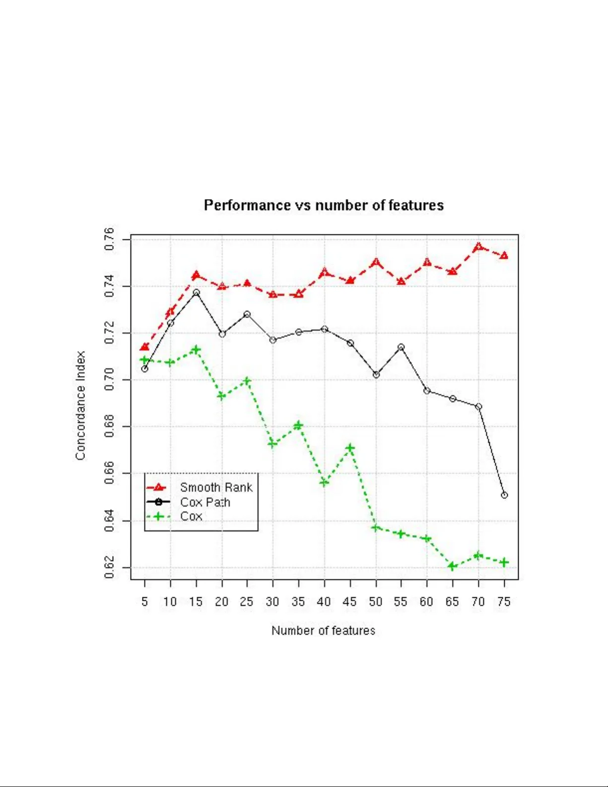
1 Ensem ble Risk Mo deling Metho d for Robust Learning on Scarce Data Marina Sapir, MetaP attern, Bar Harb or, ME ∗ E-mail: m@sapir.us Abstract In medical risk mo deling, typical data are “scarce”: they ha ve relativ ely small num ber of training instances (N), censoring, and high dimensionality (M). W e show that the problem may b e effectively simplified by reducing it to bipartite ranking, and in tro duce new bipartite ranking algorithm, Smo oth Rank, for robust learning on scarce data. The algorithm is based on ensemble learning with unsup ervised aggregation of predictors. The adv an tage of our approach is confirmed in comparison with tw o “gold standard” risk mo deling metho ds on 10 real life surviv al analysis datasets, where the new approach has the b est results on all but t wo datasets with the largest ratio N/M. F or systematic study of the effects of data scarcity on modeling b y all three metho ds, w e conducted tw o t yp es of computational exp eriments: on real life data with randomly drawn training sets of different sizes, and on artificial data with increasing n umber of features. Both exp erimen ts demonstrated that Smooth Rank has critical adv antage ov er the p opular metho ds on the scarce data; it do es not suffer from ov erfitting where other metho ds do. 1 In tro duction 1.1 The Surviv al Analysis Problem Surviv al analysis deals with datasets, where each observ ation d = h x, t, δ i includes cov ariate vector x ∈ χ , a survival time t ∈ R , t > 0 and a binary event indic ator δ ∈ { 0 , 1 } : δ = 1, if an even t (failure) o ccurred, and δ = 0 if the observ ation d is censored at time t. So, the survival time means either time to even t or to the end of study , if the observ ation was stopp ed ( c ensor e d ) without the ev ent. The last tw o v ariables represen t the tar get or outcome of the observ ation. F or example, in a study ab out risk of metastases after cancer surgery , surviv al time is time from the surgery to the discov ery of metastases, if they o ccurred, or to some other end of study . The observ ations where metastases w ere not discov ered will end up censored. The censoring ma y o ccur either b ecause the cancer was remo ved by surgery , or b ecause the patients lost to follow up b efore the cancer metastasized. Some of these lost patien ts could hav e died from different causes or mov ed to another lo cation. The prediction in surviv al analysis is generally understo od as an estimate of an individual’s risk, and the concept of risk is asso ciated not only with the fact of even t, but with its timing: the earlier the even t happ ened, the higher was the risk. Because of incomplete (censored) observ ations, the individuals in study can be partially ordered b y their risk: for observ ations d i = h x i , t i , δ i i , d j = h x j , t j , δ j i , d i ≺ d j ≡ δ i = 1 & t i < t j . Denote S : χ → R a mo del built by a surviv al analysis algorithm. The commonly accepted criterion of the risk mo deling is Harrell’s concordance index (CI) [1] b et ween the risk order ≺ and the v alues of S ( x ). The concordance index is based on the concept of c onc or dant pairs of observ ations: suc h pairs h d i , d j i , where both S ( x i ) < S ( x j ) and d i ≺ d j . The pairs, where S ( x i ) > S ( x j ) and d i ≺ d j are called disc or dant . By definition, C I = C P + 0 . 5 · T ies C P + D P + T ies, where C P , DP , T ies are n umbers of concordan t pairs, discordant pairs and ties, respectively . With con tinuos features, the ties are unlikely , and in absence of ties, concordance index measures prop ortion of concordan t pairs. 2 Th us, the goal can b e formalized as learning the partially kno wn order ≺ by the wa y of building a scoring function S ( x ) on χ to minimize the num b er of discordan t pairs of observ ations. This puts the surviv al analysis in the class of the sup ervised ranking problems (see, for example [2, 3]). What makes the problem difficult is the data quality in medical longitudinal studies, which we call “scarcit y”: the n umber of observ ations tends to b e small; many of them may b e censored; num ber of features may b e large comparing with the n umber of observ ations, the outcome and quantitativ e features dep end to a large degree on unknown factors; clinical features are sub jective; some of the features ma y b e irrelev an t - and so on. All this put main emphasis on the robustness of learning. 1.2 T raditional Approac h The surviv al analysis is not commonly treated as a ranking problem. Usually , the solution is found b y mo deling the time it takes for ev ents to occur [4, 5] (a more difficult problem), and the most common metho d for this purp ose is Cox prop ortional hazard regression (Cox PH) [6]. Cox PH regression builds a mo del b y maximizing lik eliho o d of the observed surviv al rates. Originally , the metho d was intended to study dep endence b et ween few cov ariates and the outcome; if used for prediction, it tends to ov erfit on typical data. P opular tutorial [1] recommends that num b er of co v ariates for Co x regression do es not exceed 1/10th of the n umber of uncensored observ ations. In mac hine learning, most of the developed approaches try to “improv e” Cox PH regression one wa y or another. The most p opular metho ds include L 1 or L 2 p enalization of the regression parameters [7, 8], to mak e learning more robust. As we show here on real and artificial data, this regularization may not b e sufficien t, as it often do es not lead to improv ed p erformance on scarce data and does not preven t o verfitting. 1.3 Alternativ e Approach W e prop ose an alternative approach to the surviv al analysis learning. First , we address the noise in outcome by defining the “risk” as a c hance of having failure b efore certain time T . The interpretation of risk as a prop ensit y of an individual to ha ve an early failure is natural and acceptable for medical practitioners. Considering surviv al analysis as a ranking problem and splitting observ ations on tw o classes (“early failure” vs “no early failure”) we reduce the problem to bipartite ranking (see, for example, [9]). Binarization of the surviv al outcome simplifies the problem and decreases influence of noise in the surviv al times. Let us notice, that even though only the order betw een tw o classes is mo deled, the mo del produces con tinuous scores asso ciated with the levels of risk, whic h, in turn, is related with the timing of even ts. Therefore, the p erformance still can b e ev aluated by the concordance index b et ween the scores and the order ≺ on the test data. Second , w e introduce new bipartite rank ing method Smooth Rank, designed specifically for the scarce data. The metho d is based on the str ong regularization technique used in Naive Bay es: unsup ervised aggregation of indep enden tly built univ ariate predictors. Av oiding multidimensional optimization makes Naiv e Bay es less sensitive to the “curse of dimensionality”, allo ws it to b e comp etitiv e with more sophis- ticated methods [10] on scarce data. The term str ong regularization w as first used in [4] with reference to w eighted voting [11], which is based on the same approach. In addition to the strong regularization, Smo oth Rank emplo ys smoothing techniques to mak e the mo del more robust, less dep enden t on p eculiarities of the small training samples. 1.4 Comparison of the Two Approaches T o show that our approac h is w orking, Smo oth Rank is compared here with L 1 -p enalized path metho d Co xPath and the Cox PH regression on 10 real life surviv al analysis datasets. Smo oth Rank has the b est 3 p erformance on 8 datasets. It yields to other metho ds only on the tw o datasets with the largest N / M ratio. In addition, we study relationship b et ween data scarcity and metho ds’ performance in tw o types of computations exp eriments. First, on t wo real life datasets, we randomly exclude some observ ations to pro duce series of training sets of differen t sizes. Then, on the artificial datasets, w e gradually increase the num b er of features, k eeping the size of the training set constant. Both exp eriments demonstrate that Smo oth Rank has significan t adv antage in p erformance on scarce data, while other metho ds ma y work b etter on “rich” data. 2 Smo oth Rank 2.1 Definition of Smo oth Rank The main sc heme of the algorithm can b e describ ed as tw o steps pro cedure: 1. Indep endently for eac h feature x i : build a predictor f i ( x i ) and calculate its weigh t w i based on its p erformance; 2. Calculate a scoring function F ( x ) = P n 1 w i · f i ( x i ) . F or a classification problem, there are tw o popular ensemble algorithms whic h follo w this sc heme. One of them is Naive Bay es classifier [12] where all weigh ts w i ≡ 1 and each predictor is built as a log-ratio b et w een densities of tw o classes: f i ( x i ) = l og ( d i 1 ( x i ) /d i 2 ( x i )) . Another example of an algorithm with the same sc heme is “weigh ted voting” [11]. There are several w a ys the general sc heme can b e implemen ted in the context of surviv al analysis. Belo w is one of the p ossible implemen tations. The algorithm is applied to the data, where observ ations are split on t wo classes with labels C ∈ { 1 , 2 } b y surviv al time threshold T . Bipartite Ranking Algorithm Smo oth Rank • F or each feature x i : 1. Build kernel approximations g i 1 , g i 2 of the densit y of each class on R i = dom ( x i ); 2. F or each p oint r ∈ R i calculate q i ( r ) = g i 1 ( r ) − g i 2 ( r ) π 1 · g i 1 ( r ) + π 2 · g i 2 ( r ) , where π 1 , π 2 are frequencies of the classes 1 and 2; 3. Build marginal predictors e q i ( x ) as smo oth approximation of the function q i ( x ) 4. Calculate weigh ts w i of the predictors based on their correlation with outcome • Calculate scoring function F ( x ) = X i : x i 6 = N A w i · e q i ( x i ) / X i : x i 6 = N A w i 2.2 Implemen tation and parameters The algorithm is implemen ted in R using some standard R functions. 4 2.2.1 Selection of the time threshold T In the exp erimen ts, we select the time threshold T to mak e the classes similar in size. The class 1 contains the ev ents only: d i = { x i , δ i , t i } : δ i = 1 & t i ≤ T . The class 2 contains all observ ations with the surviv al time ab o ve T . It means that the censored observ ations with censoring time below the threshold T are excluded from training. 2.2.2 Densit y ev aluation The densit y is approximated with cosine k ernel. The R function density [13] uses F ourier transform with a discretized v ersion of the k ernel and then mak es linear approximation to ev aluate the density at the sp ecified p oin ts. Density was ev aluated with default function parameters, on equally spaced 512 p oin ts. 2.2.3 Building marginal predictors The function q i ( r ) is less sensitive to the errors in the density ev aluation than the default function used in Naive Ba yes: g i 1 ( r ) /g i 2 ( r ). How ev er, for the areas where densit y of b oth classes is lo w, small errors in g i 1 , g i 2 ( r ) can lead to big errors in q i ( r ). T o deal with this issue, q i ( r ) is not ev aluated for r : π 1 · g i 1 ( r ) + π 2 · g i 2 ( r ) < 0 . 1. The aggregation on the last step handles v alues of the predictors in these p oin ts as missing. The function q i ( r ) is smo othed on the Step 3 using lo ess pro cedure with the default parameters. LOESS stands for “lo cally weigh ted scatterplot smo othing” [14]. Adv an tage of this metho d is that it does not require to sp ecify the class of functions for approximation. The pro cedure lo ess was used with p olynomials of the degree 1. 2.2.4 Calculation of w eigh ts The calculation of w eights is implemented as a tw o step pro cedure. First, w eights of the predictors are calculated by the formula w i = C I ( e q i ( x )) − 0 . 5 , where C I ( y ) is a concordance index betw een the v ariable y and the outcome. F or t wo-class outcome, in absence of ties, CI is equal area under the ROC curv e, which is common performance measure for bipartite ranking [3]. The next step includes “p ost-filtering”, or “shrink age”. The goal of this step is to impro ve learning on the datasets where man y correlated w eak predictors can ov erw eight few strong ones. Rather than setting a hard threshold for selection of predictors, or use data to optimize the threshold, the filtering is made based on comparison of all w eights with the highest w eight µ = max ( w j ). The updated weigh ts are calculated b y the formula: w i :=  w i − µ/ 3 , if w i > µ/ 3 0 , other wise. The empiric formula allows to filter out relativ ely weak predictors, making the filtering data-dep enden t without tuning of h yp er-parameters. 2.3 Prop erties of the predictors Since g i 1 , g i 2 appro ximate densities of b oth classes, according to Bay es theorem, the marginal conditional probabilit y of the class j in the p oint x i = r can b e defined by the formula: P ( Y = j | x i = r ) ' π j · g i j ( r ) π 1 · g i 1 ( r ) + π 2 · g i 2 ( r ) , 5 where Y is the class lab els, π 1 , π 2 are priors for the tw o clas ses, approximated by their frequencies. Then the marginal predictor e q i ( r ) can b e presented as e q i ( r ) ' P ( Y = 1 | x i = r ) π 1 − P ( Y = 2 | x i = r ) π 2 , difference b et ween ratios of conditional posterior probabilities to prior probabilities in tw o classes. If v ariable x i is conditionally indep enden t on Y in x i = r , b oth posterior probabilities in this p oin t are equal to their priors, and e q i ( r ) ' 0 . In each p oin t r , the v alue of marginal predictor function e q i ( r ) indicates degree and direction of lo cal asso ciation b et ween the v alues of the v ariable x i and the resp onse v ariable. Then, e q i ( r ) influences the scoring function F only for those p oin ts x i = r which are predictive, and do not participate in ranking otherwise. The fact that densities for each class are ev aluated indep enden tly increases robustness of the prop osed function. In our implemen tation, the parameters of the kernel appro ximation and LOESS procedures were fixed to ensure maximal smoothness. Th us, unlik e most of other adv anced risk mo deling methods, Smo oth Rank do es not hav e h yp er-parameters to tune up. 3 Results on Real Data 3.1 Algorithms under comparison Smo oth Rank is compared with tw o algorithms, whic h b ecome standard in surviv al analysis [4, 5, 15]. 3.1.1 Co x proportional hazard regression In the traditional approach by sir David Co x [6], risk of failure is understoo d as a time-dep enden t “hazard function” Λ( x, t ): cum ulative probability of an individual x having even t (failure) up to time t . Co x prop ortional hazard (PH) regression is based on the strong assumption that the hazard function has the form of Λ( x, t ) = λ 0 ( t ) · exp ( β ( x )) , where λ 0 ( t ) is unknown time-dependent function, common for all individuals in the p opulation. The assumption implies, in particularly , that for an y tw o individuals, their hazards are prop ortional all the time. Accordingly , the result of the mo deling is not the time-dep enden t hazard functions, but rather the “prop ortionalit y” scores. The metho d can not b e applied on data with M > N . W e use the metho d’s implementation from the R pac k age survival . The metho d do es not work with missing v alues. 3.1.2 Co xPath algorithm Co xPath [16] algorithm is one of most p opular approaches to regularization of the Co x PH regression. The path algorithm implements L 1 -p enalized Cox regression with series of v alues of regularization parameter λ . The imp ortant prop ert y of the L 1 -regularization is that it includes automatic feature selection, and it can w ork when num b er of features exceeds num b er of training cases. The function implemented in the R pack age glmp ath by the metho d’s authors is used here. The function builds regression mo dels at the v alues of λ at which the set of non-zero co efficien ts changes. F or eac h mo del, the function outputs v alues of three criteria: AIC, BIC, loglik. The criterion AIC w as c hosen to select the best mo del for the given training set. W e used default v alues of the parameters of the c oxp ath pro cedure. The metho d do es not work with missing v alues. 6 3.2 The Datasets The next datasets w ere used for metho ds comparison. • BMT: The dataset represen ts data on 137 b one marrow transplant patients [17] . The data allow to mo del sev eral outcomes. Here, the models are built for disease free surviv al time. The first feature is diagnosis, which has three v alues: ALL; AML Low Risk; AML High Risk. Other features c haracterize demographics of the patient and donor, hospital, time of w aiting for transplant, and some characteristics of the treatment. There are 11 features ov erall, among them tw o are nominal. • Colon: These are data from one of the first successful trials of adjuv an t chemotherap y for colon cancer. Lev amisole is a lo w-to xicity comp ound previously used to treat worm infestations in animals; 5-FU is a mo derately toxic (as these things go) chemotherap y agent. There is p ossibility to mo del t wo outcome: recurrence and death. The data can be found in R pack age surviv al. The features include treatmen t (with three options: Observ ation, Lev amisole, Lev amisole+5-FU); properties of the tumor, n umber of lymph no des. There are total 11 features and 929 observ ations. • Lung1: Surviv al in patien ts with adv anced lung cancer from the North Central Cancer T reatment Group [18]. P erformance scores rate ho w well the patien t can p erform usual daily activities. Other features c haracterize calories intak e and weigh t loss. The dataset has 228 records with 7 features • Lung2, the dataset from [19] Along with the patients’ performance scores, the features include cell t yp e (squamous, small cell, adeno, and large), t yp e of treatment and prior treatmen t. • BC : Breast cancer dataset [20]. It contains 7 tumor characteristics in 97 records of patients. • PBC : This data is from the May o Clinic trial in primary biliary cirrhosis of the liv er conducted b et w een 1974 and 1984 [21]. P atients are characterized by standard description of the disease conditions. The dataset has 17 features and 228 observ ations. • Al: The data [22] of the 40 patients with diffuse large B-cell lymphoma contain information ab out 148 gene expressions asso ciated with cell proliferation from lymp ohichip microarra y data. Since there are more features than the observ ations, the Cox regression could not b e applied on the data. • Ro02s: the dataset from [23] contains information ab out 240 patien ts with lymphoma. Using hierarc hical cluster analysis on whole dataset and exp ert knowledge ab out factors asso ciated with disease progression, the authors iden tified relev an t four clusters and a single gene out of the 7399 genes on the lymphochip. Along with gene expressions, the data include t w o features for histological grouping of the patients. The authors aggregated gene expressions in each selected cluster to create a signatures of the clusters. The signatures, rather than gene expressions themselves were used for mo deling. The dataset with aggregated data has 7 features. • Ro03g, Ro03s: the data [24] of 92 lymphoma patients. The input v ariables include data from lympho c hip as well as results of some other tests. The Ro03s data contain a veraged v alues of the gene expressions related with cell proliferation (proliferation signature). The Ro03g dataset includes the v alues of the gene expressions included in the proliferation cluster, instead of their a verage. Thus, the Ro03s dataset contains 6 features, and the dataset Ro03g contains 26 features. 3.3 Description of the exp erimen t F or each dataset we did 100 random splits on train and test data in prop ortion 2 : 1. F or each split, all metho ds were applied on the train data and tested on the test data. Thus, the splits are the same for all the metho ds. The p erformance of each metho d was ev aluated by av erage concordance index on the test data. 7 T able 1. Comparison of Metho ds on Surviv al Analysis Data # Data N × M N/M Smo oth Rank Co x Co x Path 1 BMT 137 × 11 12.4 0.68 (6.4) 0.58 0.58 2 Colon 929 × 11 84.4 0.65 (4) 0.66 0.66 3 Lung1 228 × 7 32.6 0.63 (5.7) 0.62 0.62 4 Lung2 137 × 6 22.8 0.73 (2.16) 0.69 0.70 5 BCW 97 × 7 13.9 0.71 (5.9) 0.69 0.69 6 PBC 418 × 17 24.6 0.83 (12.6) 0.82 0.82 7 Al 40 × 148 0.27 0.63 (110) — 0.52 8 Ro02s 240 × 7 34.3 0.70 (7) 0.73 0.73 9 Ro03s 92 × 6 15.3 0.76 (3) 0.74 0.75 10 Ro03g 92 × 26 3.54 0.76 (23) 0.58 0.67 Ev ery cell contains mean v alue of CI on the test data for 100 random splits in prop ortion 2:1. The highest v alues in each row are marked by b old font. The num b er in brack ets is a verage num ber of features left after filtering in Smo oth Rank Co x PH regression and Co xPath algorithms do not w ork with missing v alues, while Smo oth Rank do es. So, for the first tw o metho ds records with missing v alues w ere remov ed. The exception is the data Al, where there are to o few records and many missing v alues. In this dataset 5-nearest neighbors imputation w as used for all the metho ds. 3.4 The results The results are presented in the T able 1. The ratio N / M is included as some measure of the dataset scarcit y: the smaller is the ratio, the less represen tativ e (more scarce) is the dataset. F or all datasets, the table con tains av erage CI for each metho d for each dataset. The T able 1 shows that in 8 out of 10 cases Smo oth Rank has the b est results. Smo oth Rank yields to t wo other metho ds on the 2 datasets (lines 2 and 8) with the largest ratio N / M . In the three cases with the low est ratio of N / M (lines 1,7,10) the adv antage of Smo oth Rank is the most prominen t. Its p erformance is higher than p erformance of other metho ds by 9% − 11% . Let us notice that the dataset R003s is a pro cessed v ersion of the dataset Ro03g: Ro03g contains origi- nal v alues of gene expression, and Ro03s includes aggregated features, “signatures”. While Smo oth Rank has equally goo d (the best) results with or without aggregation, tw o other metho ds require preliminary feature aggregation for comparable p erformance. The table allo ws to contrast tw o types of regularization: the traditional one, with L 1- p enalization, and the prop osed here alternative approach, which includes the strong regularization. Co xPath uses p enalization and model selection to impro v e Cox PH regression, but most of times it has almost identical accuracy with Co x PH regression on the given data. A p ossible explanation is that the optimal mo del selection on the same small training set as part of the path method leads to “mo del selection bias” [25, 26]. Adv antages in accuracy of Smooth Rank o ver other metho ds indicate supe riorit y of the strong regu- larization for risk mo deling on scarce data. 4 Exp erimen ts with Con trolled Data Scarcit y T o confirm the adv antages of Smo oth Rank on scarce data, we conducted tw o series of exp eriments con trolling tw o asp ects of the data scarcity: num ber of training instances and dimensionality . In the first series with real data, some instances w ere randomly remov ed to obtain training sets of v arious sizes. In 8 the second exp erimen t on artificial data, the n umber of instances was fixed, but the num b er of features w as gradually increased. The goal was to see the trends in methods p erformance on the series of mo dified datasets. 4.1 Exp erimen ts with reduced num b er of training cases The exp erimen ts w ere conducted on tw o of the largest real life datasets from our list, PBC and Colon, where missing v alues w ere imputed using 5 nearest neighbors. F or each dataset, 20% of records were randomly selected as test data. The rest of the data were used to randomly dra w training sets of five giv en sizes, total 20 random training sets of eac h size. All the metho ds were trained on each training set and tested on the same test set. The exp eriment w as rep eated 10 times starting with selection of the test set. So, every metho d w as applied 200 times on the training sets of the same size. F or each metho d, for each sample size, av erage CI on the test data was calculated o ver all 200 mo dels. The Figures 1, 2 demonstrate trends in metho ds p erformance with increasing num b er of instances in the training set. As exp ected, av erage p erformance of eac h metho d impro ves with the num b er of training cases. In b oth cases, Smo oth Rank has higher accuracy than t wo other metho ds when training sets are small. F or the Colon dataset, as the num b er of training instances grows, CoxPH regression and Co xPath metho ds surpass in accuracy Smo oth Rank. Ov erall, the exp erimen t confirms adv antage of the Smo oth Rank on the scarce data. In particularly , on the PBC data, Smo oth Rank ac hieved the same quality of prediction, as tw o other metho ds, with ab out half of the training instances. This is an imp ortan t quality for longitudinal studies, where each individual requires mon ths or years of observ ations, making it difficult to increase the num ber of instances for learning. The exp eriment confirms our hypothesis that observed higher accuracy of Cox PH regression and Co xPath on the Colon dataset (see T able 1) can b e explained by the larger than usual size of the training sample, not some sp ecifics of the data. If only p ortion of the instances w as a v ailable, Smo oth Rank w ould b e the b est metho d to mo del the data. 4.2 Exp erimen ts with increasing num b er of features It is v ery common in surviv al analysis with medical applications that, out of all av ailable information, features for modeling are selected because they are kno wn to ha ve some b earing on the risk of failure. The artificial datasets for this exp erimen t w ere designed to mo del this type of data. First, r isk w as generated as logarithm from a normally distributed random v ariable. With the assump- tion that times of even ts t dep end on the risk and some unknown factors, the v ariable t w as generated b y the formula t = r isk + q , where q is a random v ariable with uniform distribution within interv al [ min ( r isk ) / 2 , max ( r isk ) / 2]. Half of the records w ere randomly assigned status “censored”. F or non censored observ ations (ev en ts), tar get = t. F or the censored observ ations, target times indicate the end of observ ation, whic h happened b efore the ev ent (failure) o ccurred. The target times of the censored observ ations were calculated b y form ula tar g et = t · z , where z is a random v ariable uniformly distributed within interv al [0 . 2 , 0 . 8]. Ev ery feature f was generated indep enden tly the same wa y as the times of even ts t : f = risk + q . In reality , the features do not alw ays dep end on the risk linearly . How ever, having more complex features could affect metho ds differen tly and make the effects of the dimensionality on the p erformance less clear. All exp erimen ts were conducted on the samples with 400 records, whic h were split on equally sized train and test sets. 9 Figure 1. PBC dataset 10 Figure 2. Colon dataset 11 F or each M m ultiple of 5 from the in terv al [5 , 75], training and test samples of with M features we generated 20 times. F or eac h metho d, av erage p erformance on the test was calculated for each dimension of the data. The Fig. 3. sho ws the results of the exp erimen ts. All the metho ds ha ve similar performance with the smallest num b er of features M = 5, which is equal 1/20 of the num b er of uncensored observ ations in the training set. Co x PH regression do es not benefit from adding more features. F or CoxP ath, top performance w as ac hieved with M = 15. Both Co xP ath and Co x PH regression hav e tendency of decreasing accuracy with M > 15. Smo oth Rank is the only metho d which do es not show any sign of o verfitting in this exp erimen t. It ac hieves the b est accuracy and the largest adv antage ov er other metho ds on datasets with highest studied dimensionalit y M ≥ 70. The difference in accuracy b et w een CoxP ath and Smo oth Rank for the most scarce datasets is ab out 0 . 10, whic h is similar to the results we observ ed in exp erimen ts on real data (see T able 1). The consistency b et w een the simulation and application of the metho ds on real data may serve to justify the simulation. 5 Conclusions In surviv al analysis studies with medical applications, it is muc h easier and cheaper to add features than observ ations. Unknown factors affect measuremen ts and the outcome to a large degree. Small, noisy , high-dimensional data put stringen t demands on the robustness of the learning metho ds. W e proposed tw o innov ations to address this challenge: (1) reduction of the surviv al analysis to bipartite ranking; (2) a new robust algorithm for bipartite ranking, Smo oth Rank. The metho d do es not use m ultidimensional optimization to a void the “curse of dimensionalit y”; it uses smo othing techniques while building marginal predictors. Adv antages of Smo oth Rank were prov ed exp erimen tally , in comparison against the most p opular metho ds for surviv al analysis (CoxP ath and Co x PH regression) in three types of tests. First, the three metho ds were applied on the 10 real life surviv al analysis datasets. Then, to systematically study effects of data scarcity on the methods p erformance, w e conducted tw o computational experiments: with real data, where some instances were randomly remov ed to pro duce series of training samples of different sizes, and with artificial data, where the n umber of features was gradually increased. All three types of exp eriments, indeed, demonstrated that Smo oth Rank has sizable adv antage in accuracy ov er other tw o metho ds on data with smaller num b er of observ ations and/or higher dimension- alit y . The metho d do es not suffer from ov erfitting where tw o other metho ds do. This can make the metho d a v aluable to ol in surviv al analysis studies. Smo oth Rank is a general bipartite ranking metho d. Even though its creation was motiv ated by risk mo deling, it ma y be useful in other applications where robustness of learning is critical. Comparison of the metho d with other (bipartite) ranking algorithms on other applications may b e a sub ject of another study . References 1. Harrell FE, Lee KL, Mark DB (1996) T utorai in biostatistics. multiv ariate prognostic mo dels. Statistics in Medicine 15: 361 - 387. 2. Cl´ emen¸ con S, Lugosi G, V ay atis N (2008) Ranking and empirical minimization of u-statistics. Annals of Statistics 36: 844-874. 12 Figure 3. Atrificial data 13 3. Cortes C, Mohri M (2004) Auc optimization vs. error rate minimization. In: Thrun S, Saul L, Sc h¨ olk opf B, editors, Adv ances in Neural Information Processing, Cambridge, MA: MIT Press. pp. 313 - 320. 4. Segal MR (2006) Microarray gene expression data with link ed surviv al phenotypes. Biostatistics 7: 268 - 285. 5. Wieringen W, Kun D, Hamp el R, Boulestei AL (2009) Surviv al prediction using gene expression data: a review and comparison. Computational Statistics and Data Analysis 53: 1590 - 1603. 6. Cox D (1972) Regression mo dels and life-tables. Journal of Roy al Statistical So ciet y Series B (Methological) 34: 187 - 220. 7. Gui J, Li H (2005) P enalized cox regression analysis in the high-dimensional and lo w-sample size settings, with applications to microarra y gene expression data. Bioinformatics 21: 3001 – 3008. 8. Li H, Luan Y (2003) Kernel cox regression models for linking gene expression profiles to censored surviv al data. In: Altman R, Dunker AK, Hunter L, editors, Pacific Symp osium on Bio computing, W orld Scientific. pp. 65 – 75. 9. Cl´ emen¸ con S, V ay atis N (2009) Adaptive estimation of the optimal roc curv e and a bipartite ranking algorithm. In: Galv ad` a R, Lugosi G, Zeugmann T, Zilles S, editors, Algorithmic learning theory , LNAI 5809, Springer-V erlag. pp. 216-231. 10. F riedman J (1997) On bias, v ariance, 0/1loss, and the curse-of-dimensionality . Data Mining and Kno wledge Discov ery 1: 55 – 77. 11. Golub TR, Slonim DK, T amay o P , Huard C, Gaasenbeek M, et al. (1999) Molecular classification of cancer: Class disco very and class prediction b y gene expression monitoring. Science 286: 531 - 537. 12. Hastie T, Tibshirani R, F riedman J (2009) The Elements of Statistical Learning. Springer, NY. 13. Beck er RA, Chambers JM, Wilks AR (1988) The New S Language. W adsworth and Bro oks. 14. Cleveland W (1979) Robust lo cally w eighted regression and smo othing scatterplots. Journal of the American Statistical Asso ciation 74(368): 829 – 836. 15. Raz D, Ray MR, Kim JY, He B, T aron M, et al. (2008) A multigene assay is prognostic of surviv al in patien ts with early-stage lung adeno carcinoma. Clin Cancer Res 14: 5565-5570. 16. Park M, Hastie T (2007) L1-regularization path algorithm for generalized linear models. J R Statist So c B 69: 659 - 677. 17. Klein JP , Mo esc hberger ML (2003) Surviv al Analysis: T echniques for Censored and T runcated Data. Springer, NY, 2 edition. 18. Loprinzi CL, et al (1994) Prosp ectiv e ev aluation of prognostic v ariables from patient-completed questionnaires. north central cancer treatment group. Journal of Clinical Oncology 12: 601 - 607. 19. Kalbfleisch J, Prentice R (2002) The Statistical Analysis of F ailure Time Data. J. Wiley , Hob ok en, N.J. 20. v an’t V eer LJ, et al (2002) Gene expression profiling predicts clinical outcome of breast cancer. Nature 415: 530 - 536. 14 21. Therneau T, Grambsc h P (2000) Modeling Surviv al Data: Extending the Co x Model. Springer- V erlag, New Y ork. 22. Alizadeh A, et al (2000) Distinct types of diffuse large-b-cell lymphoma identified by gene expression profiling. Nature 403: 503 – 511. 23. Rosenw ald A, et al (2002) The use of molecular profiling to predict surviv al after chemotherap y for defuse large -b-cell lymphoma. New England journal of Medicine 346: 1937 – 1947. 24. Rosenw ald A, et al (2003) The proliferation gene expression signature is a quan titative predictor of oncogenic ev ents that predict surviv al in mantle cell lymphoma. Cancer Cell : 183–197. 25. Burnham BKP , Anderson DR (1998) Mo del Selection and Multimo del Inference: A Practical- Theoretic Approac h. Springer. 26. Cawley GC, T alb ot NL (2010) On o ver-fitting in mo del selection and subsequent selection bias in p erformance ev aluation. Journal of Mac hine Learning Research 11: 2079–2107.