Efficient algorithm to select tuning parameters in sparse regression modeling with regularization

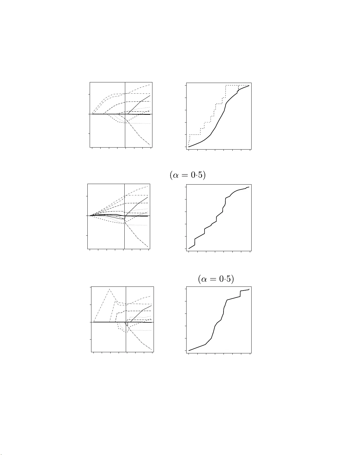
Efficien t algorithm to se l ect tuning parameters in sparse regr ession mo de ling with r e gularization Kei Hirose 1 , Shohei T ateishi 2 and Sadanor i Konishi 3 1 Division of Mathematic al Sci enc e, Gr aduate Scho ol of Engine ering Scienc e, Osaka Uni versity, 1-3, Machikaneyama-cho, T oyonaka, Osaka, 560-85 31, Jap an 2 T oyama Chemic al Co., Ltd., 3-2- 5, Nishi-Shinjuku , Shinjuku-ku, T okyo, 160-0023, Jap an. 3 F aculty of Scienc e and Engine ering, Chuo University, 1-13-27 Kasuga, Bunkyo-ku, T okyo, 112-8551, Jap an. E-mail: mail@keihir ose.c om, shohei.tateishi@gmail.c om, k onishi@math.chuo-u.ac.jp. Abstract In sparse regression mo deling via regularization suc h as the lasso, it is imp ortant to selec t appropriate v alues of tuning p arameters in cluding r egularizatio n p aram- eters. The choice of tuning parameters ca n b e view ed as a mo d el selection and ev aluation problem. Mallo ws’ C p t yp e criteria ma y b e used as a tuning param- eter selection to ol in la sso-t yp e regularization metho ds , for whic h the concept of degrees of freedom pla ys a key role. In the p resen t pap er, we pr op ose an efficien t algorithm th at compu tes the d egrees of f r eedom b y extendin g the generalized path seeking algorithm. Our pro cedure allo ws us to construct model selection criteria for ev aluating m o dels estimated by regularization w ith a w ide v ariety of con v ex and non-con v ex p enalties. Mon te Carlo s imulations demons tr ate that our metho dology p erforms w ell in v arious situations. A real data example is also giv en to illustrate our pr o cedure. Key W ords : C p , Degrees of f reedom, Generalized path seeking, Mo del selection, Regu- larization, Spar se regression, V aria ble selection 1 In t ro duction V ariable selection is fundamen tally imp ort a n t in high-dimensional linear regression mo d- eling. T raditional v ariable selection pro cedures follow the b est subset selection along with mo del selection criteria such as Ak aike ’s information criterion (Ak aik e, 1973) and the Ba y esian information criterion (Sch w arz , 1978). Ho wev er, the b est subset selection is of- ten unstable b ecause of its inherent discreteness (Breiman , 1996), and then the resulting mo del has p o or prediction accuracy . T o o v ercome this drawbac k of the subset selection, Tibshirani (1 996) prop osed the lasso, whic h shrinks some co efficien ts to w ard exactly zero b y impo sing an L 1 p enalt y on regression coefficien ts, resulting in sim ultaneous mo del selection and estimation pro cedure. 1 Ov er the past 15 y ears, there has b een a considerable amount of lasso-type p enalization metho ds in literature: bridge regression (F rank and F riedman, 1993; F u, 1 998), smo o thly clipp ed absolute deviation (F an a nd Li, 2001), elastic net (Zou a nd Hastie, 2005), gro up lasso (Y uan and Lin, 2006), a daptiv e lasso (Zo u, 2006), comp osite absolute p enalties fam- ily (Zhao et al., 2009), minimax concav e p enalty (Zhang , 2010) and g eneralized elastic net (F riedman, 2008) along with man y other r egularization t echniq ues. It is well known that the solutions are not usually expressed in a closed form, since the p enalt y term includes non-differen tiable function. A n um b er of res earc hers ha v e presen ted efficien t algorithms to obtain the en tire solutions (e.g., least angle regression, Efron et al., 2004; co ordinate descen t algorithm, F riedman et al., 2 0 07, 2010, Mazum der et al., 20 11; generalized path seeking, F r iedman, 2008). A crucial issue in the sparse regression mo deling via regularization is the selection of adjusted tuning parameters including regularization parameters , b ecause the regulariza- tion parameters iden tify a set of non-zero co efficien ts and then assign a set of v aria bles to b e include d in a mo del. Cho osing the tuning parameters can b e view ed as a mo del selection and ev aluation problem. Mallows ’ C p t yp e criteria (Mallows, 19 73) estimate the prediction e rror of t he fitted mo del, and giv e better accuracy than cross v alidation in some situations (Efron, 2004). The concept of degrees o f freedom (e.g., Y e, 1998; Efron, 1986, 200 4) pla ys a k ey role in t he theory of C p t yp e criteria. In a practical situatio n, how ev er, it is difficult to directly deriv e an analytical expres- sion o f (unbiase d estimator of ) degrees of freedom for sparse regression mo deling. A few researc hers ha v e derive d the analytical results b y using the Stein’s unbias ed risk estima- tor ( Stein , 19 81) for only sp ecific p enalties. Z ou et al. (2007) show ed that the n um b er of non-zero co efficien ts is an un biased e stimate o f the degrees of freedom of the lasso. Kato (2009) derive d an un biased estimate of the degrees fr eedom of the lasso, gro up lasso and fused la sso based on a differen tial geometric approa c h. Mazumder et al. (201 1) pro- p osed a re-parametrization of min imax conca ve p enalty , whic h e nables us to calibrate the degrees of freedom of minimax conca v e family . Ho w ev er, these se lection pro cedures do not co v er more general regularization methods via con v ex and non- con v ex p enalties. In suc h a situation, the cross v alidation and the b o otstrap (e.g., Y e, 1998; Efron, 2 0 04; Shen and Y e, 2002; Shen et a l., 2004) may b e use ful to estimate the degrees of freedom. These appro ac hes, ho w ev er, can b e computationally expensiv e, and often yield unstable estimates. In the presen t pap er, w e prop ose a new alg o rithm that can iterativ ely calculate the de- grees of freedom by extending the generalized path seeking algorithm ( F riedman, 2008). The prop osed pro cedure can b e applied to a wide v ariet y of conv ex and non-conv ex p enalties including the generalized elastic net family (F riedman, 2 008). F urthermore, our algorithm is computationally-efficien t , b ecause there is no need to p erform nume rical op- 2 timization to obtain the solutions and degrees of freedom at eac h step. The proposed metho dology is inv estigated through the analysis of r eal data and Monte Carlo sim ula- tions. Numerical results sho w that C p criterion based on our algorithm p erforms w ell in v arious situations. The remainder of this pap er is organized as follo ws: Section 2 briefly describ es the degrees of freedom in linear regression mo dels. In Section 3, w e intro duce a new algo- rithm that iterativ ely computes the degrees of freedom b y extending the generalized path seeking. Section 4 presen ts n umerical results for both artificial and real datasets. Some concluding remarks are giv en in Section 5. 2 Degrees of fre edom in linear regres sion mo dels In linear regress ion mo dels, the degrees of freedom can b e used as a model complex it y measure in Mallows’ C p t yp e criteria. Supp ose that x j = ( x 1 j , . . . , x N j ) T ( j = 1 , . . . , p ) are predictors and y = ( y 1 , . . . , y N ) T is a resp onse vec tor. Without loss of generality , it is assumed that the resp onse is cen t ered and the predictors are standardized b y c hanging a lo cation and emplo ying scale transformations N X i =1 y i = 0 , N X i =1 x ij = 0 , N X i =1 x 2 ij = 1 ( j = 1 , . . . , p ) . Consider the linear regression mo del y = X β + ε , where X = ( x 1 , . . . , x p ) is an N × p predic tor matrix, β = ( β 1 , . . . , β p ) T is a co efficien t v ector and ε = ( ε 1 , . . . , ε N ) T is a n error v ector with E [ ε ] = 0 and V [ ε ] = σ 2 I . Here I is an identit y matrix. The linear regression mo del is estimated by the p enalized least square metho d ˆ β ( t ) = argmin β R ( β ) s . t . P ( β ) ≤ t, (1) where R ( β ) is a squared erro r loss f unction R ( β ) = ( y − X β ) T ( y − X β ) / N , (2) P ( β ) is a p enalt y term whic h yields sparse solutions (e.g., the la sso p enalty is P ( β ) = P j | β j | ), and t is a tuning parameter. An equiv alent formulation of (1) is ˆ β ( λ ) = argmin β { R ( β ) + λP ( β ) } , where λ is a regularization parameter, whic h corresp onds to t in (1). 3 W e consider the problem of selecting an appropria te v alue of tuning parameter t (or λ ) b y using C p t yp e criteria, for whic h the concept of degrees of freedom plays a k ey role (Y e, 1998). Assume that the expectation and the v ariance-cov ariance matrix of the res p onse v ector y are E [ y ] = µ , V ( y ) = E [( y − µ ) ( y − µ ) T ] = τ 2 I , (3) where µ is a true mean ve ctor and τ 2 is a true v ariance. Giv en a mo deling pro cedure m , the estimate ˆ µ = m ( y ) can b e pro duced from the data v ector y . Then, the degrees of freedom o f the fitting pro cedure m is defined as (Y e, 1 998; Efron, 1986, 2004) df = N X i =1 co v( ˆ µ i , y i ) τ 2 , (4) where ˆ µ i is the i th elemen t of ˆ µ . F or example, whe n the estimator ˆ µ is expressed as a linear com binatio n of response v ector, i.e. ˆ µ = H y with H b eing indep enden t of y , the de grees of freedom is tr( H ) . The tra ce of matrix H is referred to as an effectiv e n um b er of parameters (Hastie and Tibshirani , 1990), whic h is widely used to select the tuning parameter in ridge-type regression. In sparse regression mo deling suc h as the lasso, how ev er, it is difficult to deriv e the degrees of freedom, since the p enalt y term is not differen tiable at β j = 0 ( j = 1 , . . . , p ) so that the solutions are not usually expresse d in a closed form. Mallo ws’ C p criterion, whic h is an un biased estimator of the true prediction error, can b e constructed with the degrees of freedom defined in ( 4 ). Assume that t he resp onse v ector y is generated according to (3), and the true exp ectation µ is estimated b y linear regression mo del. As a criterion to measure the effectiv eness of the mo del, w e consider the exp ected error (e.g., Hastie et al., 2008) defined by Err = E y E y new [( ˆ µ − y new ) T ( ˆ µ − y new )] , (5) where the expectation E y new is tak en o v er y new ∼ ( µ , τ 2 I ) indep enden t of y . Lemma 2.1. The exp e cte d err or in (5) c an b e expr esse d as Err = E y  k y − ˆ µ k 2 + 2 τ 2 df  . (6) Pr o of. The pro of is in App endix. Lemma 2.1 suggests C p criterion (e.g., Efron, 2004) C p = k y − ˆ µ k 2 + 2 τ 2 df , whic h is an un biased estimator o f the expected erro r in (5). The optima l mo del is selected b y minimizing C p . As a n estimator of the true v a r ia nce of τ 2 , the un biased es timator o f error v a r iance of the most complex mo del is usually used. 4 T a ble 1: Summary of mo del selection criteria based on the degrees of freedom. Criterion F orm ula C p k y − ˆ µ k 2 + 2 τ 2 df AIC N log(2 π τ 2 ) + k y − ˆ µ k 2 τ 2 + 2df AIC C N log  2 π k y − ˆ µ k 2 N  + N − 2 N df N − df − 1 BIC N log(2 π τ 2 ) + k y − ˆ µ k 2 τ 2 + log N df GCV 1 N k y − ˆ µ k 2 (1 − df / N ) 2 The degrees of freedom can lead to sev eral mo del se lection criteria, whic h a r e sum- marized in T able 1. Zou et al. (2007) intro duced Ak a ik e’s information criterion (AIC; Ak aik e, 1973) and Bay esian information criterion (BIC; Sc h w ar z, 1978). W ang et a l. (2007, 2009) sho we d that the Ba yes ian informat io n criterion holds the consistency in mo del selection. W e also in tro duce bias corrected Ak aike’s informatio n criterion (AIC C ; Sugiura, 1978; Hurvic h et al., 1998) and generalized cross v alidation (GCV; Crav en and W ah ba, 1979). These t w o criteria do not need the true v a riance τ 2 . 3 Efficien t algori t hm for co mputing the degrees of freedom In this section, first, the generalized path seeking algo r ithm is briefly described. Then, a new alg orithm that it era t ively computes the degrees of freedom is in tro duced. F ur- thermore, we mo dify the algorithm to ease the computationa l burden for large sample sizes. 3.1 Generalized path seeking algorithm F riedman (2 008) prop o sed the g eneralized pa t h seeking, whic h is a fast a lgorithm to solv e the problem (1). Th e g eneralized path seeking can pro duce the en tire solutions tha t closely appro ximate those for a wide v ariet y o f conv ex and non-conv ex constrain ts. Supp o se that the p enalty term P ( β ) satisfies follow ing condition:  ∂ P ( β ) ∂ | β j | > 0 | j = 1 , . . . , p  . (7) This condition defines a class of p enalties whe re each mem b er in the class is a mono- tone increasing function of absolute v a lue of eac h of its argumen ts. F or example, the 5 lasso penalty P ( β ) = P p j =1 | β j | is included in this class, b ecause ∂ P ( β ) /∂ | β j | = 1 > 0. Similarly , elastic net (Zou and Hastie , 20 05), group lasso (Y uan and Lin , 20 06), adaptive lasso (Z ou, 20 06), comp osite a bsolute p enalties family (Zhao et al., 2 0 09), minimax con- ca v e p enalt y (Zhang, 2010) and generalized elastic net (F riedman, 2 008) with man y other con v ex and non-conv ex p enalties are included in this class. Denote ˆ β ( t ) is the solution at tuning para meter t . The generalized path seeking algorithm s tarts at t = 0 with ˆ β (0) = 0. The solution can b e iteratively computed: for giv en ˆ β ( t ), the solution ˆ β ( t + ∆ t ) can b e pro duced, where ∆ t is a sm all p ositiv e v alue. Supp ose the path ˆ β ( t ) is a con tin uous function of t and a ll co efficien t paths { ˆ β j ( t ) | j = 1 , . . . , p } are monotone function of t , that is, {| ˆ β j ( t + ∆ t ) | ≥ | ˆ β j ( t ) | | j = 1 , . . . , p } . F o r eac h step, one elemen t of coefficien t v ector ˆ β ( t ), sa y ˆ β k ( t ), is incriminated in a correct direction λ k ( t ) with all other co efficien ts remaining unchanged, i.e. ˆ β k ( t + ∆ t ) = ˆ β k ( t ) + ∆ t · λ k ( t ) , (8) { ˆ β j ( t + ∆ t ) = ˆ β j ( t ) } j 6 = k , (9) where k and λ k ( t ) are defined as k = argmax j ∈{ 1 ,...,p } | g j ( t ) | /p j ( t ) , λ k ( t ) = g k ( t ) /p k ( t ) . (10) Here g j ( t ) and p j ( t ) are g j ( t ) = −  ∂ R ( β ) ∂ β j      β = ˆ β ( t ) , p j ( t ) =  ∂ P ( β ) ∂ | β j |      β = ˆ β ( t ) . The deriv ation of the g eneralized path seeking algorithm is in App endix. Remark 3.1. We assume d that ˆ β ( t ) is c o n tinuous a nd e ach ele ment is monotone func- tion of t . A lthough these c ondition s c an b e satisfie d in most c ases, so m etimes ˆ β ( t ) is disc ontinuous or non-mo n otone function. F rie dman (2008) pr op ose d an appr o ach f o r non-monotone c a s e, which is as f o l lows: first, we d efine a set S = { j | λ j ( t ) · ˆ β j ( t ) < 0 } . When S is not em pty, the index k is sele cte d by k = argmax j ∈ S | λ j ( t ) | . Otherwise, k = argmax j ∈{ 1 ,...,p } | λ j ( t ) | . The detaile d desc rip tion of disc ontinuous c ase is also given in F rie dman (20 0 8). When p j ( t ) = 1 ( i.e. the lasso p enalty), (8) yields ˆ β k ( t + ∆ t ) = ˆ β k ( t ) + ∆ t · g k ( t ) . (11) 6 Note that the up dated co efficien t in (8 ) and (11) mo v es in the same direction ev en if the lasso p enalt y is not applied, b ecause the condition in (7) yields sig n ( g k ( t )) = sig n ( λ k ( t )). This means that the up date equations (8) and ( 1 1) pro duce the same solution path when ∆ t → 0 unless p j ( t ) or 1 /p j ( t ) div erges. Th erefore, w e can use the up date equation in (11) instead of (8). If the up date equation in (11 ) is applied, an iterativ e algorithm tha t computes the degrees of freedom in (4) can b e deriv ed. F rom (9) and (11), the pr edicted v alue at t + ∆ t is ˆ µ ( t + ∆ t ) = ˆ µ ( t ) + ∆ t · g k ( t ) x k . (12) Because the lo ss function R ( β ) is squared loss as (2), we hav e g k ( t ) = 2 x T k ( y − ˆ µ ( t )) / N . Th us, ˆ µ ( t + ∆ t ) is ˆ µ ( t + ∆ t ) = ˆ µ ( t ) + 2 N ∆ t x k x T k · ( y − ˆ µ ( t )) . (13) Example 3.1. L et X b e ortho gona l , i.e. X T X = I . By s ubstituting (13) in to g j ( t ) = 2 x T j ( y − ˆ µ ( t )) / N , the up date e quation of g j ( t ) is g j ( t + ∆ t ) =  (1 − 2∆ t/ N ) g j ( t ) ( j = k ) , g j ( t ) ( j 6 = k ) . Be c a use of the ortho gonality, we hav e g j ( t ) = (1 − 2∆ t/ N ) t j · 2 x T j y / N , wher e t j is the numb er of times that j th c o efficient is up da te d until time step t . I t is sho w n that the absolute value of g j ( t ) is monotone non-incr e asing function and g j ( t ) → 0 when t j → ∞ . When t → ∞ , the le ast squar e d estimates c an b e obtaine d b e c ause g j ( t ) → 0 for al l j = 1 , . . . , p . 3.2 Deriv ation of up date equation of degrees of free dom Equation ( 1 3) suggests t he up date equation of the cov ariance matrix in (4) as follows : co v( ˆ µ ( t + ∆ t ) , y ) τ 2 = co v( ˆ µ ( t ) , y ) τ 2 + 2 N ∆ t x k x T k  I − co v ( ˆ µ ( t ) , y ) τ 2  . (14) The degrees of freedom is iterativ ely calculated b y taking the trace of (14 ) . The initial v alue of co v ( ˆ µ ( t ) , y ) /τ 2 is set to zero-matrix O b ecause of the follo wing equation: co v ( ˆ µ (0) , y ) τ 2 = co v(0 , y ) τ 2 = O . Let M ( t ) = cov( ˆ µ ( t ) , y ) /τ 2 and k ( t ) b e the index o f up dated elemen t of coefficien t v ector at time ste p t . The update equation of the degrees of freedom in (14) can be expresse d a s I − M ( t + ∆ t ) = ( I − α x k ( t ) x T k ( t ) )( I − M ( t )) , (15) 7 where α = 2∆ t/ N . Then, the cov ariance matrix can b e up dated b y M ( t ) = I − ( I − α x k ( t − 1) x T k ( t − 1) )( I − α x k ( t − 2) x T k ( t − 2) ) · · · ( I − α x k (1) x T k (1) ) . (16) Example 3.2. The de gr e es of fr e e dom c an b e e asily de ri v e d when X is ortho gonal. Be c ause of the ortho go n ality, the c ovaria n c e matrix in (16) c an b e c alculate d as M ( t ) = I − ( I − α x 1 x T 1 ) t 1 ( I − α x 2 x T 2 ) t 2 · · · ( I − α x p x T p ) t p = p X j =1 { 1 − ( 1 − α ) t j } x j x T j , wher e t j is define d i n Example 3.1. Then, the de gr e es of fr e e dom is tr { M ( t ) } = p X j =1 { 1 − (1 − α ) t j } . When t is very sm a l l, the de gr e es of fr e e dom is close to 0 sinc e α = 2∆ t/ N is sufficiently smal l. As t gets lar ger, the d e gr e es of fr e e dom incr e ase s sinc e (1 − α ) t j > (1 − α ) t j +1 . When t j → ∞ for al l j , the de gr e es of fr e e dom b e c omes the numb er of p ar ameters, which c oincides with the de gr e es of fr e e dom of le a s t s q uar e d es tima tes. 3.3 Mo d ification of the up date equation The up date equation in (12 ) causes little c hange in predicted v alues fro m t to t + ∆ t near the leas t squared estimates, b ecause | g k ( t ) | = | 2 x T k ( y − ˆ µ ( t )) / N | is very close to zero. In order to o v ercome this difficult y , w e update the k ( t )t h elemen t of co efficien t v ector m times. Here m is an in teger whic h becomes large near least squared estimates. Since g k ( t + ∆ t ) = (1 − 2∆ t / N ) g k ( t ) as sho wn in the Example 3.1, t he ˆ β k ( t + m ∆ t ) is ˆ β k ( t + m ∆ t ) = ˆ β k ( t ) + 1 − (1 − α ) m α ∆ t · g k ( t ) . (17) The up da t e equation in (17) can b e applied eve n when m is a p ositive real v alue. The fo llo wing up date equation can b e used so that the co efficien t is appropriately up dated near the least squared estimates: ˆ β k ( t + m ∆ t ) = ˆ β k ( t ) + ∆ t · sig n ( g k ( t )) = ˆ β k ( t ) + 1 | g k ( t ) | ∆ t · g k ( t ) . (18) Equations (17 ) and (1 8) giv e us m = log(1 − α/ | g k ( t ) | ) log(1 − α ) . (19) 8 Algorithm 1 An iterativ e algorit hm that computes the solution and the degrees of free- dom. 1: t = 0. 2: w hile {| g j ( t ) | > α } ( j = 1 , . . . , p ) do 3: Compute { g j ( t ) } and { λ j ( t ) } ( j = 1 , . . . , p ). 4: S = { j | λ j ( t ) · ˆ β j ( t ) < 0 } 5: if S = empt y then 6: k = argmax j ∈{ 1 ,...,p } | λ j ( t ) | 7: else 8: k = argmax j ∈ S | λ j ( t ) | 9: end if 10: Compute m = log ( 1 − α / | g k ( t ) | ) / log(1 − α ). 11: ˆ β k ( t + m ∆ t ) = ˆ β k ( t ) + ∆ t · sig n ( λ k ( t )) 12: { ˆ β j ( t + m ∆ t ) = ˆ β j ( t ) } j 6 = k 13: Compute M ( t + m ∆ t ) = I −  I − α t x k ( t ) x T k ( t )  ( I − M ( t )) . 14: Compute df ( t + m ∆ t ) = tr { M ( t + m ∆ t ) } 15: t ← t + m ∆ t 16: end while It should b e assumed that α < | g k ( t ) | for any step so tha t log(1 − α/ | g k ( t ) | ) exists. When m is giv en by (19), t he up date equ ation of the degrees of f r eedom in (1 5) can b e replaced with M ( t + m ∆ t ) = I −  I − α t x k ( t ) x T k ( t )  ( I − M ( t )) , (20) where α t = α / | g k ( t ) | . The algorithm that computes the solutions and the degrees of freedom is giv en in Algo rithm 1. 3.4 More efficie n t algorithm The up date equation (20) suggests eac h step costs O ( N 2 ) op erations to up date the co- v ariance matrix M ( t ). Bec ause the n um b er of iterations denoted by T is usually v ery large suc h as T = 100000, the prop osed algo rithm seems to b e inefficien t when N is la rge. Ho w ev er, a simple mo dification of the a lgorithm eases the computational burden. With the mo dified pro cess, e ac h step costs only O ( q 2 ) operat ions, w here q is the num b er of selected v a riables through the generalized pat h seeking algorithm: p − q v a riables are not selected at all steps for generalized path seek ing algorithm. When p is very large, q is 9 smaller tha n p and early stopping is used. F or example, suppose that p = 50 00; if w e do not w ant more than 200 v a riables in the final mo del, we s et q = 200 and stop the algorithm when 20 0 v ariables are selected. The mo dified a lgorithm is a s follo ws: first, the generalized path seek ing algorithm is implemen ted to obta in the en tire solutions. The degrees of freedom is not computed, whereas t he v a lue of g k ( t ) ( t = 1 , . . . , T ) should b e stored in the memory . Then, the QR decomp osition of N × q matrix X ∗ = ( x j 1 · · · x j q ) is implemen ted, where x j 1 , . . . , x j q are v ariables selected by the generalized path seeking algorithm. Note that # { j 1 , . . . , j q } = q . The matrix X ∗ can b e written as X ∗ = QR , where Q is an N × q or t hogonal matrix and R is a q × q upp er triangular mat r ix. Note that x k can be written as Q r k , where r k is the q -v ector whic h consists of k th column of R . The update equation of the degrees of freedom ba sed on (20) is tr { M ( t + m ∆ t ) } = tr { Q T M ( t + m ∆ t ) Q } = q − tr { ( I − α t r k ( t ) r T k ( t ) )( I − α t − 1 r k ( t − 1) r T k ( t − 1) ) · · · ( I − α 1 r k (1) r T k (1) ) } . (21) Therefore, the computational cost of (21) is only O ( q 2 ). W e provide a pack age msgps (Mo del Selection criteria via exte nsion of Generalized P ath Seeking), whic h computes Mallows ’ C p criterion, Ak aik e’s information criterion, Ba y esian information criterion and generalized cross v alida t ion via the degrees of fr eedom giv en in T able 1. The pack age is implemen ted in the R prog ramming system (R Dev elopment Core T eam, 2010), and av ailable from Comprehensiv e R Archiv e Netw ork (CRAN) at http://cran.r- project.org/web / p a c k a g e s / m s g p s / i n d e x . h t m l . 4 Numerical Examples 4.1 Mon te Carlo sim u lations Mon te Carlo sim ula tions w ere conducted to inv estigate the effectiv eness of o ur a lgorithm. The predictor v ectors w ere generated from Gaussian distribution with mean v ector zero. The outcome v a lues y we re generated by y = β T x + ε , ε ∼ N (0 , σ 2 ) . The following four Examples are presen ted here. 1. In Example 1, 200 data sets w ere generated with N = 20 observ ations and eigh t predictors. The true parameter w as β = (3 , 1 . 5 , 0 , 0 , 2 , 0 , 0) T and σ = 3. The pairwise correlation b et w een x i and x j w as cor( i, j ) = 0 . 5 | i − j | . 2. Example 2 w as the dense case. The mo del w a s same as Example 1, but with β j = 0 . 85 ( j = 1 , . . . , 8), and σ = 3. 10 3. The third example w as same as Example 1, but with β = (5 , 0 , 0 , 0 , 0 , 0 , 0 , 0) T and σ = 2. In this mo del, the true β is sparse. 4. In Example 4, a relativ ely large problem was considered. 200 data sets we re gener- ated with N = 1 00 observ ations a nd 40 predictors. W e set β = (0 , . . . , 0 | {z } 10 , 2 , . . . , 2 | {z } 10 , 0 , . . . , 0 | {z } 10 , 2 , . . . , 2 | {z } 10 ) T and σ = 15 . The pairwise correlation b et w een x i and x j w as cor( i, j ) = 0 . 5 ( i 6 = j ). In this sim ula t io n study , there are 3 purp o ses as follo ws: • D egrees of freedom: w e in v estigat ed whether the prop osed pro cedure can select adjusted tuning par a meters compared with the degrees of freedom of the lasso giv en b y Z ou et al. (2007). • Mo del selec tion criteria for sev eral p enalties: the p erformance of mo del selection criteria given in T able 1 w as compared for the lasso, elastic net and generalized elastic net family (F riedman, 2 008). • Sp eed: the computational time based on (20) w as compar ed w ith that based on (21). A detailed description of eac h is presen ted. Degrees of freedom W e compared the degrees of freedom computed by our pro cedure (df g ps , where g ps means generalized path seeking) with the degrees of freedom of the lasso prop osed b y Zou et al. (2007) ( df z ou ). The degrees of freedom of the la sso is the n um b er of non-zero co efficien ts. Our metho d and Zou’s et al. (2007) pro cedure do not yield iden tical result, sinc e the df z ou is a n un biased estimate of the degree s of freedom while df g ps is the exact v alue of the degrees of freedom. In this simulation study , the true v alue of τ 2 w as used to compute the mo del selection criteria. T a ble 2 sho ws the result of mean squared error (MSE) and the standard deviation (SD), which are the mean and standard deviation of the follow ing squared error (SE): S E ( s ) = 1 N k ˆ µ ( s ) − X β k 2 where ˆ µ ( s ) is the estimate of predicted v alues for s th dataset. The prop ortio n of cases where zero (non-zero) co efficien ts cor r ectly set to zero (non-zero), sa y , ZZ (NN), w as also computed. W e can see that 11 T a ble 2 : Mean squared error (MSE), the standard deviation (SD ) and the p ercen tage of cases where zero ( no n-zero) co efficien ts correctly set to zero (non- zero), sa y , ZZ (NN), for our prop osed pro cedure (df g ps ) and Z ou et al. ( 2007) (df z ou ). Ex. 1 Ex. 2 Ex. 3 Ex. 4 df g ps df z ou df g ps df z ou df g ps df z ou df g ps df z ou MSE 2.498 2.732 2.7 6 1 3.202 0.759 0.790 41.35 42 .37 SD 1.468 1.726 1 .3 53 1.727 0.577 0.647 10.67 1 2.36 ZZ 0.59 2 0.667 — — 0 .607 0.767 0 .5 86 0.636 NN 0.925 0.892 0.706 0.64 9 1.000 1.00 0 0.689 0.653 • Our pro cedure sligh tly outp erfo r med Z ou’s et al. (2007) one in terms of minimizing the mean squared error f o r all examples. • Z ou’s et al. (2007 ) pro cedure selected zero co efficien t s correctly than t he prop o sed pro cedure, while our metho d correctly detected non-zero co efficien ts compared with the Zou’s et al. (2007) approa ch. This means our pro cedure tends to incorp orate man y mor e v ariables than the Zou’s et al. (2007) one. Mo d el selection criteria for sev eral p enalties W e compared the p erformance o f mo del selection criteria ba sed on the degrees of freedom: C p criterion ( C p ), bias corrected Ak aik e’s informatio n criterion (AIC C ), Bay esian infor- mation criterion (BIC) and g eneralized cross v alidatio n (GCV). Because C p criterion and Ak aik e’s information criterion (AIC) yield the same results when true error v ariance τ 2 is giv en, the result of Ak aike’s info rmation criterion is not presen ted in t his pap er. F or C p criterion and Ba y esian information criterion, w e need to estimate the true erro r v ariance τ 2 . The v alue of τ 2 w as estimated by the ordinary least squares of most complex mo del. The cross v alidatio n, w hic h is one o f the most p opular metho ds to select the tuning pa- rameter in sparse regression via regularization, w as also applied. Since the leav e-one-out cross v alida t ion is computationally exp ensiv e, the 10-fold cross v alida t ion w as used. In this simu lation study , we also compared the feature a nd performance of sev eral p enalties including t he lasso, elastic net and g eneralized elastic net. The elastic net and generalized elastic net are giv en as follows: 1. Elastic net: P ( β ) = p X j =1  1 2 αβ 2 j + (1 − α ) | β j |  , 0 ≤ α ≤ 1 . 12 Here α is a tuning parameter. Note that α = 0 yields the lasso, and α = 1 pro duces the ridge p enalt y . 2. G eneralized elastic net: P ( β ) = p X j =1 log { α + (1 − α ) | β j |} , 0 < α < 1 , where α is the tuning parameter. F riedman (2008) sho w ed the g eneralized elastic net a ppro ximates the p o w er family p enalties P ( β ) = P | β j | γ (0 < γ < 1), whereas the differe nce occurs at ve ry small absolute co efficien ts. The detailed description of the generalized elastic net is in F riedman (2008). A similar idea of generalized elastic net is in Cand` es et al. (2008). Note that the degrees of freedom of the lasso (Zou’s et al., 20 07) cannot b e directly applied to the generalized elastic net family . W e computed mean squared erro r (MSE), standard deviation (SD), the prop ortion of cases where zero ( no n-zero) co efficien ts correctly set to zero (non-zero), sa y , ZZ (NN). T a bles 3, 4 and 5 sho w the comparison of mo del selection criteria for the lasso, elastic net ( α = 0 . 5) and generalized elastic net ( α = 0 . 5 ) . The detailed discussion of eac h example is as f o llo ws: • The generalized elastic net yie lded the sparsest solution, while the elastic net pro- duced the densest one. In Example 2, i.e. the dense case, the elastic net p erformed v ery w ell. On the other hand, in sparse case (Example 3), the generalized elastic net most o ften selected zero co efficien ts corr ectly . • In most cases, bias corrected Ak a ike’s information criterion (AIC C ) resulted in go o d p erformance in terms o f mean squ ared error. The Ba yes ian information criterion (BIC) p erformed v ery w ell in some cases (e.g., Examples 3 and 4 on the lasso). In dense cases (Example 2), ho w ev er, the p erformance of Ba y esian informatio n criterion (BIC) w as p o or. • The p erformance of cross v alidation (CV) for generalized elastic net family w as excellen t on Example 3. On Examples 1, 2 and 4 , how ev er, the mean squared erro r w as large compared with other mo del selection criteria based on the degrees o f freedom. The cross v alidat io n estimates expected error b y separating the training data from the test data. Unfortunately , the r egula rization metho d with non-conv ex p enalt y suc h as g eneralized elastic net does not pro duce unique solution: small c hange in the training data can result in differen t solution. Th us, the cross v alidation ma y b e unstable f o r non-conv ex p enalt y in man y cases. 13 T a ble 3: Comparison of mo del selection criteria fo r the lasso. C p AIC C GCV BIC CV Ex. 1 MSE 2 .604 2.497 2.614 2.56 7 2.905 SD 1 .562 1.463 1 .583 1.50 0 1.722 ZZ 0.51 9 0 .562 0.49 8 0.622 0.605 NN 0.925 0 .923 0.93 5 0.918 0.903 Ex. 2 MSE 2 .807 2.772 2.781 2.89 1 3.195 SD 1 .435 1.399 1 .420 1.46 2 1.712 ZZ — — — — — NN 0.733 0 .729 0.75 0 0.678 0.686 Ex. 3 MSE 0 .855 0.790 0.879 0.74 4 0.986 SD 0 .666 0.601 0 .673 0.59 4 0.692 ZZ 0.54 3 0 .573 0.52 4 0.639 0.716 NN 1.000 1 .000 1.00 0 1.000 1.000 Ex. 4 MSE 4 1.66 42.91 43.82 39.2 2 43.59 SD 1 0.72 11.19 1 1.74 9.51 2 11.83 ZZ 0.57 7 0 .545 0.53 0 0.671 0.643 NN 0.692 0 .704 0.71 3 0.653 0.655 T a ble 4: Comparison of mo del selection criteria fo r the elastic net ( α = 0 . 5). C p AIC C GCV BIC CV Ex. 1 MSE 2 .860 2.814 2.826 2.93 3 3.017 SD 1 .520 1.487 1 .533 1.55 2 1.556 ZZ 0.06 6 0 .088 0.06 1 0.101 0.074 NN 0.995 0 .993 0.99 5 0.993 0.997 Ex. 2 MSE 2 .199 2.061 2.169 2.21 8 2.301 SD 1 .434 1.303 1 .352 1.48 9 1.432 ZZ — — — — — NN 0.973 0 .967 0.97 6 0.958 0.964 Ex. 3 MSE 1 .566 1.675 1.577 1.71 4 1.720 SD 0 .754 0.834 0 .755 0.87 8 0.960 ZZ 0.01 4 0 .031 0.01 6 0.036 0.028 NN 1.000 1 .000 1.00 0 1.000 1.000 Ex. 4 MSE 2 5.15 23.31 25.55 24.7 3 24.73 SD 1 0.51 8.656 1 1.27 9.03 1 9.431 ZZ 0.00 0 0 .000 0.00 0 0.000 0.000 NN 1.000 1 .000 1.00 0 1.000 1.000 14 T a ble 5: Comparison of mo del selection criteria for the g eneralized elastic net ( α = 0 . 5 ). C p AIC C GCV BIC CV Ex. 1 MSE 3 .060 2.996 3.051 3.11 2 3.785 SD 1 .825 1.810 1 .835 1.82 1 2.015 ZZ 0.70 9 0 .776 0.69 5 0.811 0.792 NN 0.798 0 .778 0.81 3 0.752 0.707 Ex. 2 MSE 3 .757 3.747 3.658 4.01 8 4.411 SD 1 .638 1.587 1 .619 1.67 1 2.108 ZZ — — — — — NN 0.502 0 .462 0.51 7 0.416 0.457 Ex. 3 MSE 0 .889 0.803 0.949 0.68 3 0.485 SD 0 .773 0.722 0 .780 0.69 0 0.641 ZZ 0.71 4 0 .749 0.67 9 0.805 0.859 NN 1.000 1 .000 1.00 0 1.000 1.000 Ex. 4 MSE 7 4.68 74.12 75.15 78.7 5 80.56 SD 1 8.22 17.97 1 8.90 16.1 9 22.41 ZZ 0.79 6 0 .796 0.76 6 0.912 0.815 NN 0.379 0 .382 0.40 8 0.262 0.352 15 T a ble 6: Computatio na l time (se conds) base d on up date equation (20) (na ¨ ıv e) and (21) (mo dified) a v eraged ov er 200 runs for the lasso. Ex. 1 Ex. 2 Ex. 3 Ex. 4 na ¨ ıv e mo dified na ¨ ıv e mo dified na ¨ ıve mo dified na ¨ ıv e mo dified N = 10 0 1.399 0.145 1.434 0.164 1.3 98 0.143 1 .521 0.34 3 N = 20 0 4.827 0.190 4.8 34 0.246 4 .820 0.188 5.012 0.37 5 N = 50 0 69.92 0.313 69 .96 0.351 6 9.89 0.310 70.38 0.45 9 Sp eed The computational time based on up date equation (20) (na ¨ ıv e update) was compared with that based on (2 1) (mo dified update). In order to compare the timings for v arious n um b er of samples, w e c hang ed the n umber of samples N f o r all Examples: N = 100, 200 a nd 50 0. T able 6 sho ws t he result of timings av eraged ov er 20 0 runs for la sso p enalt y . All timings w ere carried out on an In tel Core 2 Duo 2.0 GH processor on Mac OS X. Note that the “ timing” means the c omputational time of pro ducing the solutions and computing the mo del selection criteria. The sp eed based on na ¨ ıv e up date was ve ry slow when N = 50 0 , b ecause w e need O (500 2 ) op erations to compute the degree of freedom for eac h step. How ev er, the modified algorithm w as fast ev en when the n um b er of samples w as lar g e. 16 T a ble 7: The estimated standardized co efficien ts for the diab etes data based on the lasso, elastic net ( α = 0 . 5) and g eneralized elastic net ( α = 0 . 5). (In tercept) a g e sex bmi map tc ldl hdl tc h ltg g lu lasso 152 0 − 209 52 2 3 03 − 120 0 − 224 12 5 18 58 enet 152 − 2 − 220 504 309 − 93 − 81 − 188 122 460 87 genet 152 0 − 228 53 2 3 26 0 − 70 − 288 0 48 9 0 4.2 Application to diab etes data The prop osed algo rithm was applied to diab etes dat a (Efron et al., 2004), whic h has N = 442 and p = 10. T en baseline predictors include age, sex, b o dy mass index (bmi), a v erage blo o d pressure (bp), and six blo o d serum measuremen t s (tc, ldl, hdl, tch , lt g , glu). The resp onse is a quan titative measure of disease progression one year after baseline. W e considered the f ollo wing three p enalties: the lasso, elastic net ( α = 0 . 5), and generalized elastic net ( α = 0 . 5). The en t ir e solution path alo ng with the solution selected b y C p criterion, and the degrees of f reedom ar e presen ted in Figure 1. On the lass o p enalty , the degrees of freedom of the lasso (Zou et al., 2007) is also depicted. The de grees of freedom of our pro cedure was smaller than that of the lasso (Zo u et al., 2 0 07) except for k ˆ β ( t ) k ∈ [2838 , 2 851], whe re the degrees of freedom of the lasso decreased because the non-zero co efficien t of 7th v ariable b ecame zero at t = 2838. On the elastic net p enalt y with α = 0 . 5, the degrees of freedom increase d rapidly at some p oints. F or example, when k ˆ β ( t ) k = 343 . 76, the degree s of freedom increase d b y ab out 0.86 4. Figure 2 sho ws the solution path of 2nd v ariable and g 2 ( t ), whic h is helpful for understanding wh y the degrees of freedom rapidly increased. When k ˆ β ( t ) k attained 343 . 76, t he sign of g 2 ( t ) changed. A t this p oin t, ˆ β 2 ( t ) > 0. Thus , g 2 ( t ) ˆ β 2 ( t ) < 0 a t k ˆ β ( t ) k = 343 . 76, whic h means ˆ β 2 ( t ) w as up dated b ecause the set S in line 4 in Algorithm 1 b ecame S = { 2 } . When | g ( t ) | w as sufficien tly small, m in (19) b ecame v ery large, whic h made a substan tial c hange in the degrees of freedom. The estimated standa r dized co efficien ts for the dia b etes da t a based on the lasso, elastic net ( α = 0 . 5) and generalized elastic net ( α = 0 . 5 ) are rep orted in T a ble 7. The tuning parameter was selected by C p criterion, where the degrees o f freedom w as computed via the pro p osed pro cedure. The generalized elastic net yielded the sparsest solution. On the other hand, the elastic net did not pro duce sparse solutio n. 17 lasso elastic net generalized elastic net 0 500 1500 2500 3500 ï 0 500 |beta| Standardiz ed coefficients 0 500 1500 2500 3500 ï 0 500 1000 |beta| Standardiz ed coefficients 0 500 1500 2500 3500 ï 0 500 |beta| Standardiz ed coefficients 0 500 1500 2500 3500 0 2 4 6 8 10 |beta| df 0 500 1500 2500 3500 0 2 4 6 8 10 |beta| df 0 500 1500 2500 3500 0 2 4 6 8 10 |beta| df Figure 1: The solution path (left panel) a nd the de grees of freedom (righ t panel). The v ertical line in the solutio n path indicates the selec ted mo del by C p criterion. The solid line o f upp er right panel is the degrees of freedom of the lasso (Zou et al., 2007) 18 |beta| |beta| Figure 2: The solution path β 2 ( t ) (left pa nel) and g 2 ( t ) (righ t panel) of the 2nd v ariable for elastic net with α = 0 . 5. 19 5 Conclud ing Remarks W e hav e prop osed a new pro cedure for selecting tuning parameters in sparse regres- sion modeling via regularization, for whic h the degrees of freedom w as calculated b y a computationally-efficien t algorithm. Our pro cedure can b e applied to construct mo del se- lection criteria f or ev aluat ing mo dels estimated by the regularization metho ds with a wide v ariet y of con v ex and non-con v ex p enalties. Mon te Carlo sim ulations w ere conducted to in v estigate the effectiv eness of the prop o sed pro cedure. Although the cross v alidation has b een widely us ed to select tuning parameters, the mo del selection c riteria based on the degrees of free dom often yielde d b etter results, esp ecially for non-con v ex p enalties suc h as generalized elastic net. In the presen t pap er, w e considered a computat io nally-efficien t algorithm t o select the tuning parameter in the sparse regression mo del. F or more general mo dels including gen- eralized linear mo dels, m ultiv ariate a nalysis such as factor analysis and graphical mo dels, it is also imp ortant to select appropriate v alues of tuning parameters. As a future researc h topic, it is in teresting to in t r o duce a new selection algorithm tha t handles large mo dels b y unifying the mathematical approac h a nd computational a lgorithms. App endix Pro of of Lemma 2.1 First, we divide k y new − ˆ µ k 2 in to three terms as follows: k y new − ˆ µ k 2 = k y new − µ k 2 + k µ − ˆ µ k 2 + 2( y new − µ ) T ( µ − ˆ µ ) . (A1) The term k µ − ˆ µ k 2 is expressed as k µ − ˆ µ k 2 = k y − ˆ µ k 2 + k y − µ k 2 − 2( y − µ ) T ( y − ˆ µ ) = k y − ˆ µ k 2 − k y − µ k 2 + 2( y − µ ) T ( ˆ µ − µ ) = k y − ˆ µ k 2 − k y − µ k 2 + 2( y − µ ) T ( ˆ µ − E y [ ˆ µ ]) +2( y − µ ) T ( E y [ ˆ µ ] − µ ) . (A2) Substituting ( A2) in to (A1) giv es us k y new − ˆ µ k 2 = k y new − µ k 2 + k y − ˆ µ k 2 − k y − µ k 2 + 2( y − µ ) T ( ˆ µ − E y [ ˆ µ ]) +2( y − µ ) T ( E y [ ˆ µ ] − µ ) + 2( y new − µ ) T ( µ − ˆ µ ) . By taking expectation of E y new , w e o bta in E y new [ k y new − ˆ µ k 2 ] = E y new [ k y new − µ k 2 ] + k y − ˆ µ k 2 − k y − µ k 2 20 +2( y − µ ) T ( ˆ µ − E y [ ˆ µ ]) + 2 ( y − µ ) T ( E y [ ˆ µ ] − µ ) . Equation (6) can b e deriv ed b y taking the exp ectation of E y and using E y new [ k y new − µ k 2 ] = E y [ k y − µ k 2 ] = nτ 2 . Deriv ation of genera lized path seeki ng algorithm W e deriv e the generalized path seeking alg orithm. First, the follow ing lemma is pro vided. Lemma 5.1. L et us c onsider the fol lowin g pr oblem. ∆ ˆ β ( t ) = argmin ∆ β [ R ( ˆ β ( t ) + ∆ β ) − R ( ˆ β ( t ))] s . t . P ( ˆ β ( t ) + ∆ β ) − P ( ˆ β ( t )) ≤ ∆ t. (A3) The solution is ∆ ˆ β ( t ) = ˆ β ( t + ∆ t ) − ˆ β ( t ) . Pr o of. The constraint in (A3) is written as P ( ˆ β ( t ) + ∆ β ) ≤ P ( ˆ β ( t )) + ∆ t ≤ t + ∆ t. Assume that β ∗ = ˆ β ( t ) + ∆ β . The n, the problem ( A3 ) is ˆ β ∗ = argmin β ∗ [ R ( β ∗ )] s . t . P ( β ∗ ) ≤ t + ∆ t. The solution is ˆ β ∗ = ˆ β ( t + ∆ t ), whic h leads to ∆ ˆ β ( t ) = ˆ β ( t + ∆ t ) − ˆ β ( t ). When ∆ t is sufficien tly small, the problem (A3) can b e a ppro ximately written as ∆ ˆ β ( t ) = argmax { ∆ β j | j =1 ,...,p } p X j =1 g j ( t ) · ∆ β j (A4) s . t . X ˆ β j ( t )=0 p j ( t ) · | ∆ β j | + X ˆ β j ( t ) 6 =0 p j ( t ) · sig n ( ˆ β j ( t )) · ∆ β j ≤ ∆ t. (A5) Since all co efficien t paths { ˆ β j ( t ) | j = 1 , . . . , p } are monotone functions of t , w e hav e { sig n ( ˆ β j ( t )) = sig n (∆ ˆ β j ( t )) | j = 1 , . . . , p } . Therefore, the problem in (A5) can b e expresse d a s ∆ ˆ β ( t ) = argmax { ∆ β j | j =1 ,...,p } p X j =1 g j ( t ) · ∆ β j s . t . p X j =1 p j ( t ) · | ∆ β j | ≤ ∆ t. (A6) The problem in (A6) can b e view ed as a line ar programming. Then, the up dates in (8) and (9) can b e derived . 21 References Ak aik e, H. (1973 ) , “Information theory and a n extension of the maxim um lik eliho o d principle,” in 2nd Int. S ymp . on Information The ory , Ed. B. N. P etrov and F. Csaki, pp. 267– 81. Buda p est: Ak ademiai Kia do. Breiman, L . (1996), “Heuristics of instability and stabilization in mo del selection,” A nn. Statist. , 24, 23 50–2383. Cand ` es, E., W akin, M., and Boy d, S. (200 8), “Enhancing Sparsit y b y Rew eigh ted ℓ 1 Minimization,” J. F ourier. A nal. Appl. , 14 , 877–905. Cra v en, P . and W ahba, G. (1979), “Smo othing noisy data with spline functions: Esti- mating the correct degree o f smo othing by the metho d of generalized cross-v alida tion,” Numer. Math. , 31, 377–403. Efron, B. (1986), “How bia sed is the apparent erro r rate of a prediction rule?” J. Am. Statist. Asso c. , 81, 461–470 . — (2 0 04), “ The estimation of prediction error: co v a riance p enalties a nd cross-v a lidation,” J. Am. Statist. Asso c. , 99, 619– 6 42. Efron, B., Hastie, T., Johnstone, I., a nd Tibs hirani, R. ( 2004), “Least angle regression (with discussion),” A nn. Statist. , 32 , 407–499. F an, J. and Li, R . (2001), “V ariable selection via nonconca v e p enalized lik eliho o d and its oracle prop erties,” J. Am. Statist. Asso c. , 9 6, 1348–1 360. F rank, I. and F riedman, J. (1993), “A Statistical View of Some Chemometrics Regression T o ols,” T e chnometrics , 35, 10 9 –148. F riedman, J. (2008), “F ast sparse regression and classification,” T ech. rep., Stanford Re- searc h Institute, California. F riedman, J., Ha stie, H., H¨ ofling, H., and Tibshirani, R. (2007), “P athw ise co ordinate optimization,” Ann. Appl. Statist. , 1, 30 2 –332. F riedman, J., Hastie, T., and Tibshirani, R . (2010), “Regularization paths f or generalized linear mo dels via co ordinate descen t,” J. Stat. Softwar e , 33. F u, W. (1998 ) , “P enalized regression: the bridge v ersus the lasso,” J. Comput. Gr a ph. Statist. , 7, 397 –416. Hastie, T. and Tibshirani, R. (1990 ), Gener alize d A dditive Mo dels , Chapman and Hall/CR C Monographs on Statistics and Applied Probability . 22 Hastie, T., Tibshirani, R ., a nd F r iedman, J. (2 008), T he Ele m ents of Statistic al L e arning , New Y ork: Springer, 2nd ed. Hurvic h, C. M., Simonoff , J. S., a nd Tsai, C.-L. (19 9 8), “Smo othing parameter selection in nonparametric regression using an impro v ed Ak aike information criterion,” J. R. Statist. So c. B , 60, 271–293 . Kato, K. (2009), “On the degrees of freedom in shrink age estimation,” J. Multivariate A nal. , 10 0 , 1338–13 52. Mallo ws, C. (1973), “Some commen ts on C p ,” T e chnom etrics , 661–6 7 5. Mazumder, R., F riedman, J., and Hastie, T. (20 11), “ SparseNet: Coordina t e descen t with non-con v ex p enalties,” J. A m. Statist. Asso c . , 106 , 1125–1138. R Dev elopmen t Core T eam (2010), R: A L an guage an d Envir onm e nt for Statistic al Com- puting , R F oundatio n for Stat istical Computing, Vienna, Austria, ISBN 3- 900051- 07-0. Sc h w ar z, G. (1978), “Estimation o f the mean o f a m ultiv ariate normal distribution,” A nn. Statist. , 9, 113 5–1151. Shen, X., Huang, H.-C., and Y e, J. (2004), “Adaptiv e mo del selection and a ssessmen t for exp o nen tial family mo dels,” T e chn ometrics , 46, 306–3 17. Shen, X. and Y e, J. (2002), “Adaptiv e mo del selection,” J. Amer. Statist. Asso c. , 97, 210–221. Stein, C. (1981 ), “Estimation of the mean of a m ultiv ariate normal distribution,” Ann. Statist. , 9, 113 5–1151. Sugiura, N. (1978), “F urther analysis of the da t a b y Ak aik e’s informatio n criterion and the finite corr ections,” Commun. Statist. A.-The or. A. , 7, 13–2 6. Tibshirani, R. (1996), “Regression shrink age and selec tion via the lasso,” J. R. Statist. So c. B , 58, 267–288 . W a ng, H., Li, B., and Leng, C. ( 2 009), “Shrink age tuning parameter selection with a div erging n umber of parameters,” J. R. Statist. So c. B , 71, 671–68 3. W a ng, H., Li, R., and T sai, C. (2007 ), “T uning parameter s electors for the smoothly clipp ed a bsolute deviation metho d,” Bi o metrika , 94, 55 3 –568. Y e, J. (1 998), “On measuring a nd correcting the effects of data mining and mo del selec- tion,” J. Amer. Statist. Asso c. , 93, 1 20–131. 23 Y uan, M. a nd Lin, Y. (2006), “ Mo del selection and estimation in regression with group ed v ariables,” J. R. Statist. So c. B , 68, 4 9–67. Zhang, C. (201 0 ), “Nearly un biased v ariable selec tion under minimax conca v e penalty ,” A nn. Statist. , 38, 894–942. Zhao, P ., Ro c ha, G., and B., Y. (200 9), “The composite absolute p enalties family for group ed a nd hierarc hical v aria ble selection,” A nn. Statist. , 37, 34 68–3497. Zou, H. (2006 ), “The adaptive Lasso and its oracle prop erties,” J. A mer. Statist. Asso c. , 101, 1418 –1429. Zou, H. and Hastie, T. (2005), “Regular izat io n a nd v ariable selection via the elastic net,” J. R. Statist. So c. B , 67, 301–320. Zou, H., Hastie, T., and Tibshirani, R. (2007), “On the D egrees of F reedom of the La sso,” A nn. Statist. , 35, 2173–2192. 24