Discriminant Analysis with Adaptively Pooled Covariance

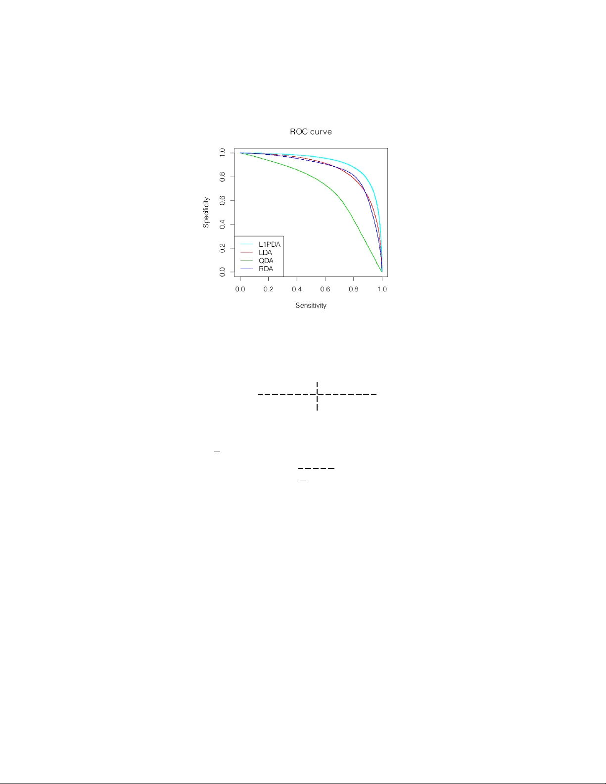
DISCRIMINANT ANAL YSIS WITH AD APTIVEL Y POOLED CO V ARIANCE NO AH SIMON AND R OB TIBSHIRANI Abstra ct. Linear and Quadratic Discriminan t analysis (LDA/QD A) are common to ols for classification problems. F or these metho ds w e assume observ ations are normally distributed within group. W e estimate a mean and co v ariance matrix for each group and classify using Bay es theorem. With LD A, we estimate a single, p o oled co- v ariance matrix, while for QD A w e estimate a separate cov ariance matrix for each group. Rarely do we b elieve in a homogeneous co v ariance structure betw een groups, but often there is insufficient data to separately estimate co v ariance matrices. W e prop ose ` 1 - PD A, a regularized model which adaptively p o ols elements of the precision matrices. A daptively p o oling these matrices decreases the v ariance of our estimates (as in LDA), without ov erly biasing them. In this pap er, we prop ose and discuss this metho d, give an efficien t algorithm to fit it for mo derate sized problems, and show its efficacy on real and simulated datasets. Keywor ds : Lasso, Penalized, Discriminant Analysis, In terac- tions, Classification 1. Intr oduction Consider the usual tw o class problem: our data consists of n ob- serv ations, each observ ation with a known class lab el ∈ { 1 , 2 } , and p co v ariates measured p er observ ation. Let y denote the n -vector corre- sp onding to class (with n 1 observ ations in class 1 and n 2 in class 2 ), and X , the n b y p matrix of co v ariates. W e w ould like to use this information to classify future observ ations. W e further assume that, given class y ( l ) , eac h observ ation, x l , is inde- p enden tly normally distributed with some class sp ecific mean µ y ( l ) ∈ R p and co v ariance Σ y ( l ) , and that y ( l ) has prior probability π 1 of coming from class 1 and π 2 from class 2 . F rom here we estimate the t w o mean v ectors, co v ariance matrices, and prior probabilites and use these esti- mates with Ba y es theorem to classify future observ ations. In the past a num b er of differen t metho ds hav e b een prop osed to estimate these parameters. The simplest is Quadratic Discriminant Analysis (QD A) 1 2 NO AH SIMON AND R OB TIBSHIRANI whic h estimates the parameters by their maximum likelihoo d estimates π k = n k n ˆ µ k = 1 n k X y ( l )= k x l and ˆ Σ k = 1 n k X y ( l )= k ( x l − µ k ) ( x l − µ k ) > . T o classify a new observ ation x , one finds the class with the highest p osterior probability . This is equiv alen t in the tw o class case to con- sidering D ( x ) = log  π 1 π 2  − 1 2 ( x − µ 1 ) > Σ − 1 1 ( x − µ 1 ) + 1 2 ( x − µ 2 ) > Σ − 1 2 ( x − µ 2 ) + logdet  Σ − 1 / 2 1 Σ 1 / 2 2  and if D ( x ) > 0 then classifying to class 2 , otherwise to class 1 . Linear Discriminan t Analysis (LD A) is a similar but more commonly used metho d. It estimates the parameters by a restricted MLE — the co v ariance matrices in b oth classes are constrained to b e equal. So, for LD A ˆ Σ 1 = ˆ Σ 2 = 1 n n X l =1  x l − µ y ( l )   x l − µ y ( l )  > While one rarely believes that the cov ariance matrices are exactly equal, often the decreased v ariance from p o oling the estimates greatly out- w eigh ts the increased bias. F riedman [1989] prop osed Regularized Discriminan t Analysis (RD A) noting that one can partially p o ol the cov ariance matrices and find a more optimal bias/v ariance tradeoff. He estimates Σ k b y a con vex com bination of the LDA and QDA estimates ˆ Σ k = λ ˆ Σ QDA k + (1 − λ ) ˆ Σ LDA where λ is generally determined by cross-v alidation. W e extend the idea of partially p o oling the co v ariance matrices in a differen t direction. W e make the further assumption that for most i, j ,  Σ − 1 1  i,j ≈  Σ − 1 2  i,j ; that the partial cov ariance matrices are mostly DISCRIMINANT ANAL YSIS WITH AD APTIVEL Y POOLED COV ARIANCE 3 elemen t-wise equal (or nearly equal). In tuitiv ely this sa ys that condi- tional on all other v ariables, most pairs of cov ariates in teract iden tically in b oth groups. Giv en this assumption, the natural approac h is to find a restricted MLE where the n um b er of non-zero entries in Σ − 1 1 − Σ − 1 2 is constrained to b e less than some c . ie. to find argmax ` 1 ( µ 1 , Σ 1 ) + ` 2 ( µ 2 , Σ 2 ) s.t.   Σ − 1 1 − Σ − 1 2   0 ≤ c Σ 1 , Σ 2 P ositiv e Semi-Definite where ` k is the Gaussian log likelihoo d of the observ ations in class k , ` k ( µ k , Σ k ) = − n k 2 log(2 π )+ n k 2 logdet  Σ − 1 k  + X y ( l )= k ( x l − µ k ) > Σ − 1 k ( x l − µ k ) and k · k 0 is the num ber of nonzero elemen ts. Unfortunately , this prob- lem is not conv ex and would require a com binatorial searc h. Instead w e consider a conv ex relaxation argmax ` 1 ( µ 1 , Σ 1 ) + ` 2 ( µ 2 , Σ 2 ) (1) s.t.   Σ − 1 1 − Σ − 1 2   1 ≤ c (2) Σ 1 , Σ 2 P ositiv e Semi-Definite (3) where k · k 1 is the sum of the absolute v alue of the en tries. Because the | · | is not differentiable at 0 , solutions to (1) hav e few nonzero entries in Σ − 1 1 − Σ − 1 2 with the sparsit y level dep enden t on c . There is a large liter- ature about using ` 1 p enalties to promote sparsit y (Tibshirani [1996], Chen et al. [1998], among others), and in particular sparsit y has been applied in a similar framew ork for graphical mo dels [Banerjee et al., 2008]. Also recently , a very similar model to that whic h we prop ose has been applied to joint estimation of partial dep endence among man y similar graphs [Danaher et al., 2011]. The astute reader may note that (1) is not join tly con v ex in µ and Σ − 1 . Ho w ev er, w e can still find the global maxim um — for fixed µ 1 and µ 2 it is conv ex, and, as w e later sho w, our estimates of µ 1 and µ 2 are completely indep enden t of our estimates of Σ 1 , and Σ 2 . The problem (1) has an equiv alen t Lagrangian form (whic h w e will write as a minimization for future conv enience) argmin − ` 1 ( µ 1 , Σ 1 ) − ` 2 ( µ 2 , Σ 2 ) + λ   Σ − 1 1 − Σ − 1 2   1 (4) s.t. Σ 1 , Σ 2 P ositiv e Semi-Definite (5) 4 NO AH SIMON AND R OB TIBSHIRANI This is the ob jectiv e which we will fo cus on in this pap er. W e will call its solution “ ` 1 P o oled Discriminant Analysis” ( ` 1 -PD A). F or λ = 0 these are just QD A estimates and for λ sufficiently large, just LDA estimates. In this pap er, w e examine the ` 1 -PD A ob jective; we discuss the connections betw een ` 1 -PD A and estimating interactions in a logistic mo del; we show the efficacy of ` 1 -PD A on real and simulated data; and w e giv e an efficien t algorithm to fit ` 1 -PD A based on the alternating direction metho d of momen ts (ADMM). 1.1. Reductions. One ma y note that our ob jectiv e (4) is not join tly con v ex in µ k and Σ k , how ev er this is not a problem (the optimization splits nicely). F or a fixed Σ 1 , µ ∗ 1 minimizes 1 2 X y ( l )=1 ( x l − µ 1 ) > Σ − 1 1 ( x l − µ 1 ) . This is true iff Σ − 1 1 X y ( l )=1 ( x l − µ ∗ 1 ) = 0 . Th us, µ ∗ 1 = ¯ x 1 = 1 n 1 P y ( l )=1 x l is the sample mean from class 1 , and similarly µ ∗ 2 is the sample mean from class 2 . W e can simplify our ob jectiv e (4) b y substituting the sample means in for µ ∗ 1 and µ ∗ 2 and noting that X y ( l )=1 ( x l − ¯ x 1 ) > Σ − 1 1 ( x l − ¯ x 1 ) = 1 2 X y ( l )=1 tr h ( x l − ¯ x 1 ) > Σ − 1 1 ( x l − ¯ x 1 ) i = n 1 X y ( l )=1 tr h Σ − 1 1 ( x l − ¯ x 1 ) ( x l − ¯ x 1 ) > /n 1 i = n 1 tr   Σ − 1 1 X y ( l )=1 ( x l − ¯ x 1 ) ( x l − ¯ x 1 ) > /n 1   = n 1 tr  Σ − 1 1 S 1  . where ˆ Σ 1 is the sample cov ariance matrix for class 1 . Our new ob jective is min Σ 1 , Σ 2 − n 1 logdet  Σ − 1 1  + n 1 tr(Σ − 1 1 S 1 ) − n 2 logdet  Σ − 1 2  (6) + n 2 tr(Σ − 1 2 S 2 ) + λ || Σ − 1 1 − Σ − 1 2 || 1 (7) sub ject to Σ 1 and Σ 2 p ositiv e semi-definite (PSD). This is a jointly con v ex problem in Σ − 1 1 and Σ − 1 2 . DISCRIMINANT ANAL YSIS WITH AD APTIVEL Y POOLED COV ARIANCE 5 2. Solution Pr oper ties There is a v ast literature on using ` 1 norms to induce sparsity . In this section we will insp ect the optimality conditions for our particular problem to gain some insight. W e b egin b y reparametrizing ob jectiv e (17) in terms of ∆ =  Σ − 1 1 − Σ − 1 2  / 2 , and Θ =  Σ − 1 1 + Σ − 1 2  / 2 min ∆ , Θ − n 1 logdet (∆ + Θ) + n 1 tr([∆ + Θ] S 1 ) − n 2 logdet (Θ − ∆) (8) + n 2 tr([Θ − ∆] S 2 ) + λ || ∆ || 1 (9) T o find the Karush-Kuhn optimalit y conditions, we take the subgradi- en t of this expression and set it equal to 0 . W e see that (10) − n 1  ˆ ∆ + ˆ Θ  − 1 + n 1 S 1 − n 2  ˆ Θ − ˆ ∆  − 1 + n 2 S 2 + λ∂ ( ˆ ∆) = 0 and (11) − n 1  ˆ ∆ + ˆ Θ  − 1 + n 1 S 1 + n 2  ˆ ∆ − ˆ Θ  − 1 − n 2 S 2 = 0 where ˆ ∆ and ˆ Θ minimize the ob jectiv e and ∂ (∆) is a p b y p matrix with ∂ (∆) i,j = ( sign (∆) i,j , if ∆ i,j 6 = 0 ∈ [ − 1 , 1] , if ∆ i,j = 0 No w, we can substitute Σ − 1 1 and Σ − 1 2 bac k in to the subgradien t equa- tions: (12) n 1  S 1 − ˆ Σ 1  − n 2  S 2 − ˆ Σ 2  + λ∂ ( ˆ Σ − 1 1 − ˆ Σ − 1 2 ) = 0 and (13) S po ol ≡ n 1 S 1 + n 2 S 2 n 1 + n 2 = n 1 ˆ Σ 1 + n 2 ˆ Σ 2 n 1 + n 2 . W e find these optimality conditions curious as they directly inv olv e ˆ Σ k rather than ˆ Σ − 1 k . Equation (12) sho ws that the solution will hav e a sparse difference ˆ Σ − 1 1 − ˆ Σ − 1 2 . Though somewhat unintuitiv e, it parallels the KKT conditions for the Lasso and other ` 1 p enalized problems. In particular, b ecause the subgradient of k ∆ k 1 can tak e a v ariety of v alues for ∆ i,j = 0 , the optimality conditions are often satisfied with ∆ i,j = 0 for man y i, j . Equation (13) sho ws us that the p o oled av erage of our estimates is unchanged ( S po ol = ˆ Σ po ol ). Giv en the form of our p enalt y w e find it interesting that the p o oled a v erage of the ˆ Σ k is constant (in- dep enden t of λ ) rather than some conv ex combination of the ˆ Σ − 1 k . 6 NO AH SIMON AND R OB TIBSHIRANI F rom these optimality conditions one can easily find the optimal so- lutions at b oth ends of our path (for λ = 0 and λ sufficien tly large). If S 1 and S 2 are full rank, then for λ = 0 the optimality conditions are satisfied by the QDA solution with ∂ = 0 , and for λ > λ textrmmax ≡ n 1 n 2 k S 1 − S 2 k ∞ / ( n 1 + n 2 ) the conditions are satisfied by the LD A so- lution with ∂ = n 1 n 2 ( S 1 − S 2 ) / [ λ ( n 1 + n 2 )] . In Section 5, w e give a path wise algorithm to fit ` 1 -PD A along our path of λ -v alues from λ max to 0 . 2.1. When is the problem ill posed? Recall that if S 1 or S 2 is not full rank, then the QDA solution is undefined. In our case one can see that as λ → 0 w e still ha ve this difficulty , how ev er for λ > 0 , so long as S po ol = ( n 1 S 1 + n 2 S 2 ) / ( n 1 + n 2 ) is full rank, our solution is w ell defined. In the case that S po ol is not full rank, then the solution is ill-defined for all λ . 3. F or w ard Vs Ba ckw ard Model So far w e ha v e assumed a model in which the x -v alues are gener- ated given the class assignmen ts. W e will henceforth refer to this as the “bac kward generative mo del” or backw ard mo del. Man y other ap- proac hes to classification use a “forw ard generative mo del” wherein w e consider the class assignmen ts to b e generated from the x-v alues (eg. logistic regression). Our backw ard mo del has a corresp onding forward mo del. By Bay es theorem we ha v e P( y = 1 | x ) = π 1 exp ( l 1 ) π 2 exp ( l 2 ) + π 1 exp ( l 1 ) = exp [log( π 1 /π 2 ) + l 1 − l 2 ] 1 + exp [log( π 1 /π 2 ) + l 1 − l 2 ] where l k = − ( x − ˆ µ k ) > ˆ Σ − 1 k ( x − ˆ µ k ) / 2 . W e can simplify this to get a better handle on it. Some algebra gives us logit [P( y = 1 | x )] = log ( π 1 /π 2 ) + µ > 2 Σ − 1 2 µ 2 / 2 − µ > 1 Σ − 1 1 µ 1 / 2 (14) +  Σ − 1 1 µ 1 − Σ − 1 2 µ 2  > x + x >  Σ − 1 2 − Σ − 1 1  x/ 2 . (15) where logit( p ) = p/ (1 − p ) . This is just a logistic mo del with in terac- tions and quadratic terms. In general a logistic mo del tak es the form logit [P( y = 1 | x )] = β 0 + X β i x i + X i ≤ j γ i,j x i x j DISCRIMINANT ANAL YSIS WITH AD APTIVEL Y POOLED COV ARIANCE 7 or in matrix form (16) logit [P( y = 1 | x )] = β 0 + β > x + x > Γ x/ 2 So our forward generative mo del in (14) is a logistic mo del with β 0 = log( π 1 /π 2 ) + µ > 2 Σ − 1 2 µ 2 / 2 − µ > 1 Σ − 1 1 µ 1 / 2 β = Σ − 1 1 µ 1 − Σ − 1 2 µ 2 Γ / 2 = Σ − 1 2 − Σ − 1 1 Note, that with LD A we estimate Γ to b e identically 0 , with QDA Γ is entirely nonzero, and with ` 1 -PD A, Γ has both zero and nonzero elemen ts. 3.1. Estimating In teractions. Based on the forward mo del abov e, one can consider our sparse estimation of Γ as a metho d for estimating sparse in teractions. There has b een a recent push to estimate in ter- actions in the high dimensional setting (Radchenk o and James [2010], Zhao et al. [2009], among others). The basic idea is to consider a general logistic mo del as in (16) (or a linear mo del for con tin uous resp onse), and to estimate β 0 , β , and Γ in such a wa y that there are few nonzero en tries in ˆ Γ (often the diagonal is constrained to be 0 ). The simplest of these approaches maximize a p enalized logistic log-lik eliho o d argmax β , Γ n X i =1  y ( l ) log ( p l ) + (1 − y ( l )) log(1 − p l )  − λ || Γ || 1 s.t. log  p l 1 − p l  = β 0 + β > x l + x > l Γ x l / 2 As we hav e sho wn, for discriminant analysis considered as a forw ard mo del, nonzero off-diagonal terms in Γ = ˆ Σ − 1 2 − ˆ Σ − 1 1 corresp ond to pairs of v ariables with interactions. Th us ` 1 -PD A estimates a logistic mo del with sparse in teractions (and quadratic terms). ` 1 -PD A differs from other metho ds b ecause it has additional distributional assumptions on the cov ariates which in turn put constrain ts on our estimates of β 0 , β , and Γ , but the underlying idea is the same. 3.2. Linear V s Quadratic Decision Boundaries. The sparsity of Γ again sho ws up if w e consider the decision boundaries of discriminant analysis. F or eac h metho d (LDA, QD A and ` 1 -PD A), once the param- eters are estimated, R p is partitioned into tw o connected spaces — one space where the estimated p osterior probability of an observ ation is higher for class 1 and another space where it is higher for class 2 . The decision b oundary is D = { x | P( y = 1 | x ) = 0 . 5 } whic h is equiv alen t to 8 NO AH SIMON AND R OB TIBSHIRANI { x | logit [P( y = 1 | x )] = 0 } . Referring bac k to our forward generative framew ork, (14), we see that D = n x    ˆ β 0 + ˆ β > x + x > ˆ Γ x = 0 o The nonzero terms in ˆ Γ = ˆ Σ − 1 2 − ˆ Σ − 1 1 corresp ond to pairs of dimensions in whic h the decision b oundary is quadratic rather than linear. As ex- p ected, LDA has a linear decision b oundary , and QDA has a quadratic decision b oundary (with all cross terms included). ` 1 -PD A is a h ybrid of these — it is quadratic in some terms and linear in others. 4. Comp arisons A n umber of other methods ha v e b een prop osed for discriminan t analysis using sparsity and p o oling. These methods are useful, but fill a differen t role than ` 1 -PD A. W e will compare 2 of these ideas to ` 1 -PD A and discuss when each is appropriate. 4.1. RD A. Regularized Discriminan t Analysis [F riedman, 1989] esti- mates the within class cov ariance matrices as a conv ex com bination of the LD A and QDA estimates. Lik e ` 1 -PD Ait gives a path from LDA to QD A. In con trast RD A is basis equiv ariant (changing the basis on whic h you train will not change the predictions), while ` 1 -PD A is not. In RDA, one uses a common idea in empirical ba yes and stein estima- tion — w e often o verestimate the magnitude of extreme effects, in our case we ov erestimate the extremit y of largest and smallest eigenv alues of Σ 1 − Σ 2 , so RDA shrinks these v alues. On the other hand, ` 1 -PD A is v ery basis sp ecific. In ` 1 -PD A, as in all sparse signal pro cessing, we b eliev e we hav e a go o d basis (in our case, w e b elieve that the differ- ences are sparse in this basis) and w ould lik e to lev erage this in our estimation. 4.2. Sparse LDA. A num b er of metho ds hav e b een prop osed for “sparse LD A.” (Dudoit et al. [2002], Bic k el and Levina [2004], Witten and Tibshirani [2011], among others). These metho ds either assume diagonal cov ariance matrices and lo ok for sparse mean differences, or assume Σ 1 = Σ 2 and (either implicitly or explicitly) lo ok for sparsit y in Σ − 1 ( µ 1 − µ 2 ) . This gives a linear decision rule which uses only few of the v ariables. These metho ds are well suited to very high dimensional problems (they require many fewer observ ations than LDA). In contrast ` 1 -PD A do es not remo v e v ariables — it only shrinks de- cision b oundaries from quadratic to linear. It is not well suited to very high dimensional problems. In particular, the solution is degenerate if DISCRIMINANT ANAL YSIS WITH AD APTIVEL Y POOLED COV ARIANCE 9 p > n 1 + n 2 , but it will generally p erform better than sparse LDA for p < n 1 + n 2 . T o draw another parallel to logistic regression (as in Section 3.1), Sparse LDA is similar to sparse estimation of main effects (with no in- teractions), while ` 1 -PD A is similar to sparse estimation of interactions (with all main effects included). 5. Optimiza tion One of the main attractions of this criterion is that it is a conv ex problem and hence a global optimum can b e found relatively quickly . In particular we ha v e dev elop ed a metho d whic h can solv e this for up to sev eral h undred v ariables (though the accuracy in p o orly conditioned larger problems can b e an issue). First, for ease of notation we introduce n ew v ariables: let A = Σ − 1 1 , B = Σ − 1 2 , S A = S 1 , and S B = S 2 . If w e plug in the sample means for µ 1 and µ 2 , our new criterion (negated for conv enience) is no w min A,B − n 1 logdet A + n 1 tr( AS A ) − n 2 logdet B (17) + n 2 tr( B S B ) + λ || A − B || 1 (18) sub ject to A , B PSD, where n 1 is the num b er of observ ations in group 1 , n 2 is the num ber of observ ations in group 2 . Recall that this is con- v ex in A and B . One could solve this using interior p oint metho ds discussed in Bo yd and V andenberghe [2004]. Unfortunately , for semi-definite programs the complexit y of interior point algorithms scales lik e p 6 , making this approac h i mpractical for p larger than 15 or 20 . Instead w e develop an approach based on the alternating direction metho d of moments (ADMM) which scales up to sev eral hundred co v ariates. 5.1. ADMM Algorithm. ADMM is an older class of algorithms which has recen tly seen a re-emergence largely thanks to Bo yd et al. [2010]. Our particular algorithm is a adaptation of their ADMM algorithm for sparse inv erse cov ariance estimation. The motiv ation for this algo- rithm is simple — the com bination of a logdet term and a || · || 1 term mak es our optimization difficult, so w e split the 2 up and in troduce an auxiliary v ariable C ≡ A − B and a dual v ariable Γ . W e lea v e the details of developing this algorithm to the app endix (though they are straigh tforw ard). The exact algorithm is (1) Initialize A 0 , B 0 , C 0 , and Γ 0 and choose a fixed ρ > 0 10 NO AH SIMON AND R OB TIBSHIRANI (2) Iterate until con vergence (a) Update A by A k +1 = U ˜ AU > where ρ ( C k + B k + Γ k ) − n 1 S A = U D U > is its eigen v alue decomp osition (with D = diag ( d i ) ), and ˜ A is diagonal with ˜ A ii = d i + p d 2 i + 4 ρn 1 2 ρ (b) Update B by B k +1 = V ˜ B V > where ρ ( A k +1 − C k − Γ k ) − n 2 S B = V E V > is its eigen v alue decomp osition (with E = diag ( e i ) ) and ˜ B is diagonal with ˜ B ii = e i + p e 2 i + 4 ρn 2 2 ρ (c) Update C b y C k +1 = S λ/ρ ( A k +1 − B k +1 − Γ k ) where S λ ( · ) is the element-wise soft thresholding op erator S λ ( Z ) i,j = sign ( Z i,j ) max ( | Z i,j | − λ, 0) (d) update Γ by Γ k +1 = Γ k + ρ ( C k +1 − A k +1 + B k +1 ) Up on conv ergence, A ∗ and B ∗ are the v ariables of in terest (the rest ma y b e discarded). The complexit y of each step of this algorithm is dominated b y the eigen v alue decomp ositions, eac h of whic h require O ( p 3 ) op erations. 6. P a th-wise Solution Often we do not kno w a-priori what v alue our regularization param- eter should be and w ould lik e to fit the entire path from λ max (corre- sp onding to the LD A solution) to λ = 0 (corresp onding to the QDA solution). W e define λ max ≡ n 1 n 2 k S 1 − S 2 k ∞ n 1 + n 2 It is easy to see that for λ ≥ λ max , ˆ Σ 1 = ˆ Σ 2 = n 1 S 1 + n 2 S 2 n 1 + n 2 (our LD A solution) satisfies (10) and (11), and thus is our solution. One can also see that ˆ Γ = n 1 n 2 ( S 1 + S 2 ) n 1 + n 2 is our optimal dual v ariable for λ ≥ λ max . DISCRIMINANT ANAL YSIS WITH AD APTIVEL Y POOLED COV ARIANCE 11 T o solv e along a path w e start at λ = λ max , and plug in our kno wn solution. W e then decrease λ and solve the new problem, initializing our algorithm at the previous ˆ Σ 1 , ˆ Σ 2 , and ˆ Γ . Because λ changes only sligh tly (and thus our solution changes only slightly), this approach is v ery efficient as compared to solving from scratc h at each λ . When S A and S B are full rank our QDA solution is well defined and it is p ossible to run our path all the w ay to λ = 0 . Due to conv ergence issues along the p otentially p o orly conditioned end of the path (which w e discuss in the next section) w e instead c ho ose to set λ min = λ max and log-linearly in terp olate b et ween the t w o (in our implementation default  v alue is 0 . 01 ). 6.1. Con v ergence Issues. While ADMM is a go od algorithm for find- ing an near exact solution, it is not considered a great algorithm for an exact solution (though it do es even tually conv erge to arbitrary tol- erance, this ma y require an un wieldy n um b er of iterations). In our application, solving to mac hine tolerance is unnecessary (the statisti- cal uncertainties are m uc h greater than this). How ev er, in some cases (esp ecially with p ∼ n 1 + n 2 ), near the end of the path our solution con v erges extremely slowly . Unfortunately there is no simple fix for this (more accurate interior p oint algorithms don’t scale b eyond 15 or 20 v ariables). While not ideal, this do es not ov erly concern us — con- v ergence is slow in the region where Σ − 1 1 − Σ − 1 2 is not very sparse (a region where we exp ect ` 1 -PD A to perform po orly an yw a ys). W e will see an example of this issue arise later in Section 8. One should also note that con v ergence rates near the end of the path are highly dep endent on our choice of ρ . This is c haracteristic of all ADMM problems. T o date, finding a disciplined choice of ρ for ADMM is still an op en question. W e use ρ = 1 as our default, as it app ears to w ork reasonably well for a range of problems. 7. Simula ted and Real D a t a T o sho w its efficacy , w e applied ` 1 -PD A to real and sim ulated data. In b oth cases w e compare our metho d to linear, quadratic and regular- ized discriminant analysis and sho w improv emen t ov er b oth in o v erall classification error and on R OC plots. In all problems ` 1 -PD A was fit with 30 lambda v alues log-linearly in terp olating λ max and 0 . 01 ∗ λ max . RD A w as fit with 30 equally spaced λ -v alues b etw een 0 and 1 . 7.1. Sim ulated Data. W e sim ulated data from the t wo class gaussian mo del describ ed in Section 1 with p = 30 cov ariates. W e set Σ 1 = I p × p 12 NO AH SIMON AND R OB TIBSHIRANI Figure 1. A v erage ROC curve for simulated data with n k = 33 , c = 0 . 9 and Σ 2 =  C 0 0 I ( p − 5) × ( p − 5)  where C is 5 × 5 matrix with constan t v alue c on the off diagonal en tries, and 1 on the diagonal. W e also set a small mean difference b etw een the groups: µ 1 = 0 p µ 2 =  ∆ 0 ( p − 10)  where ∆ is a 10 -vector of 1 s Under this mo del Σ − 1 1 − Σ − 1 2 is nonzero only in the upp er left 5 × 5 submatrix. W e simulated using v arying num b ers of observ ations n 1 = n 2 ∈ (33 , 40 , 60) , and v alues of c ∈ (0 . 3 , 0 . 6 , 0 . 9) . W e used 3 data sets for each sim ulation — one to fit the initial mo del, one to choose the optimal v alue of λ and our final set to get an unbiased estimate of misclassification error. As you can see from T able 7.1, when the signal to noise ratio (SNR) is to o small ` 1 -PD A adaptiv ely shrinks to w ards LD A and sees similar p er- formance. When SNR is sufficiently large (the third group in the table), ` 1 -PD A is able to pick out the nonzero en tries and ac hiev es substan- tially b etter misclassification rates. In these cases RDA also do es fairly w ell (adaptiv ely c ho osing b etw een LDA and QDA), how ev er b ecause it DISCRIMINANT ANAL YSIS WITH AD APTIVEL Y POOLED COV ARIANCE 13 # Observ ations p er Group ( n k ) 33 40 60 c = 0.3 ` 1 -PD A 0.82 0.85 0.88 LD A 0.82 0.85 0.88 QD A 0.58 0.65 0.74 RD A 0.81 0.85 0.88 c = 0.6 ` 1 -PD A 0.82 0.83 0.87 LD A 0.82 0.84 0.86 QD A 0.59 0.66 0.76 RD A 0.81 0.83 0.86 c = 0.9 ` 1 -PD A 0.84 0.88 0.92 LD A 0.80 0.83 0.85 QD A 0.65 0.76 0.86 RD A 0.81 0.84 0.88 T able 1. A v erage % of correct classifications ov er 100 sim ulated datasets (standard errors for all entries are less than 0 . 006 ) do es not tak e sparsit y in to account, it is outp erformed b y ` 1 -PD A. W e consider the large SNR case more carefully in Figure 1 (an ROC curve for n k = 33 , c = 0 . 9 ) Again we used 3 data sets p er realization to get an unbiased curve estimate (and ran 100 random realizations, though only av erage is sho wn on Figure 1). W e estimated AUC for eac h pro- cedure: ` 1 -PD A 0 . 924 ± 0 . 002 , LD A 0 . 875 ± 0 . 003 , QD A 0 . 732 ± 0 . 007 , and RD A 0 . 887 ± 0 . 003 . ` 1 -PD A do es substan tially better than LD A, QD A, and RDA. With p = 30 and n k = 33 there is clearly not enough data for QD A to p erform w ell (though the sample correlation matrices are still inv ertible). How ev er, as noted, ` 1 -PD A also has a large edge o v er LD A and RD A. 14 NO AH SIMON AND R OB TIBSHIRANI 0 5 10 15 20 25 30 0.65 0.70 0.75 0.80 0.85 0.90 % Of Correctly Classified Obs in V alidation Set Index of Lambda % Correctly Classified L1PD A LD A QD A RD A 0.2 0.4 0.6 0.8 1.0 0.0 0.2 0.4 0.6 0.8 1.0 ROC curve Sensitivity Specificity L1PD A LD A QD A RD A Figure 2. Plot of v alidated prediction accuracy for reg- ularization path in 58 mines/ro cks, with λ min = 0 . 01 λ max for ` 1 -PD A, and R OC curv e for λ 11 8. Real D a t a W e also applied ` 1 -PD A to the “Sonar, Mines vs. Ro c ks” data [Gor- man and Sejnowski, 2010]. This dataset has 60 sonar signals measured on each of 208 ob jects (eac h lab eled as either a ro c k or a mine). W e randomly chose 150 Mines/Ro cks to train with, and then classified the remaining 58 . As one can see from Figure 2, ` 1 -PD A p erforms b etter on this data than either LD A, QDA or RDA. Estimated true classification rate p eaks near the middle of our regularization path, showing that a fair amoun t of regularization can significan tly impro v e classification. As we men tioned in Section 6.1 one can see conv ergence issues near the end of our path — we would expect the CV error at our 30th λ -v alue to nearly matc h that of QD A (nearly rather than exactly b ecause w e don’t run to λ min = 0 ). Ho w ev er, it do es not, indicating that our solution is not con v erging to the QDA solution. This do es not ov erly concern us as our v alidation error reaches its crest w ell b efore this. W e also see an ROC curve comparing ` 1 -PD A, LDA, QDA, and RDA. F or RDA we c hose the simplest mo del which maximized predictive ac- curacy (the 21 st λ v alue), and for ` 1 -PD A the tenth λ v alue, the most regularized mo del b efore a precipitous drop in predictiv e accuracy (so as to minimize bias for ` 1 -PD A). The ` 1 -PD A curv e ma y still b e sligh tly DISCRIMINANT ANAL YSIS WITH AD APTIVEL Y POOLED COV ARIANCE 15 biased as w e chose it from a section of our path seen to do well in ov er- all classification error (though not the p eak). Nonetheless, this curv e app ears indicative of an adv an tage from ` 1 -PD A o ver LDA, QD A, and RD A. 9. Discussion In this pap er w e prop osed ` 1 -PD A, a classification metho d for gauss- ian data which adaptiv ely p o ols the precision matrices. W e motiv ated our metho d, and sho w ed connections b et ween it and estimating sparse in teractions. W e gav e tw o efficient algorithms to fit ha ve ` 1 -PD A, and ha v e shown its efficacy on real and simulated data. W e ha ve made and plan to pro vide an R implemen tation for ` 1 -PD A publically av ailable on CRAN. 10. Appendix α W e include a short o v erview of the ADMM algorithm. W e can rewrite (17) as min A,B − n 1 logdet A + n 1 tr( AS A ) − n 2 logdet B + n 2 tr( B S B ) + λ || C || 1 s.t. C = A − B A t the optim um w e ha ve C = A − B , so this is equiv alen t to min A,B ,C − n 1 logdet A + n 1 tr( AS A ) − n 2 logdet B (19) + n 2 tr( B S B ) + λ || C || 1 + ρ 2 k C − A + B k 2 F (20) s.t. C = A − B (21) ρ can b e an y fixed p ositive num b er (though its c hoice will affect the con v ergence rate of algorithm). W e will motiv ate this addition shortly . No w, using strong dualit y , w e can mov e our con train t into the ob jective, and finally arrive at max Γ min A,B ,C − n 1 logdet A + n 1 tr( AS A ) − n 2 logdet B (22) + n 2 tr( B S B ) + λ || C || 1 + ρ trace  Γ > ( C − A + B )  (23) + ρ 2 k C − A + B k 2 F (24) 16 NO AH SIMON AND R OB TIBSHIRANI F or ease of notation w e denote ψ Γ ( A, B , C ) = − n 1 logdet A + n 1 tr( AS A ) − n 2 logdet B + n 2 tr( B S B ) + λ || C || 1 + ρ trace  Γ > ( C − A + B )  + ρ 2 k C − ( A − B ) k 2 F and M (Γ) = min A,B ,C ψ Γ ( A, B , C ) . No w, by basic con v ex analysis, the dual of an y strongly conv ex function (with conv exit y constant ρ ) is differentiable and its deriv ativ e has lips- c hitz constant ρ . Unfortunately (19) is not necessarily strongly conv ex, ho w ever the addition of || C − A + B || 2 F , affords it many of the same prop erties. In particular if C ∗ , A ∗ , B ∗ are the argmin of ψ Γ 0 for a giv en Γ 0 , then ∂ ∂ Γ M     Γ 0 = C ∗ − A ∗ + B ∗ If w e could easily calculate M (Γ) , then we could use gradien t ascent on Γ Γ k +1 = Γ k + ρ ( C ∗ k − A ∗ k + B ∗ k ) and one w ould ha v e A ∗ k and B ∗ k con v erging to the argmax of our original problem (4). Unfortunately , M (Γ) is not easy to calculate, how ev er ψ Γ is relatively simple to minimize in one v ariable at a time ( A , B , or C ) with all other v ariables fixed. In ADMM we employ the same idea as gradien t descen t, only w e fudge the details — instead of actually calculating M (Γ) , we minimize first in A , with B , and C fixed, then in B with A and C fixed and finally in C with A and B fixed. After these 3 up dates, we take our “gradient” step as b efore (though this time it is not a true gradient step). This leads to the following algorithm: (1) Initialize A 0 , B 0 , C 0 , and Γ 0 (2) Iterate until con vergence (a) Update A by A k +1 = argmin A ψ Γ k ( A, B k , C k ) (b) Update B by B k +1 = argmin B ψ Γ k ( A k +1 , B , C k ) (c) Update C b y C k +1 = argmin C ψ Γ k ( A k +1 , B k +1 , C ) (d) T ak e “gradient step”; up date Γ b y Γ k +1 = Γ k + ρ ( C k +1 − A k +1 + B k +1 ) DISCRIMINANT ANAL YSIS WITH AD APTIVEL Y POOLED COV ARIANCE 17 One may note that if w e instead iterate steps a − c to con v ergence eac h time b efore taking step d , we end up again with gradien t descent. 10.1. Inner Lo op Up dates. In this section we derive the exact up- dates for A , B , and C in steps a, b and c of ou r ADMM algorithm. W e b egin with A : to find argmin A ψ Γ k ( A, B k , C k ) we must minimize − n 1 logdet A + n 1 tr( AS A ) + ρ trace  Γ > k ( C k − A + B k )  + ρ 2 | C k − A + B k k 2 F If we take the deriv ative of this and set it equal to 0 we get (25) ρA − n 1 A − 1 = ρ ( C k + B k + Γ k ) − n 1 S A No w if w e let ρ ( C k + B k + Γ k ) − n 1 S A = U D U > b e its eigen v alue decomp osition (with D = diag ( d i ) ), then (25) is satisfied by A = U ˜ AU > where ˜ A is diagonal and ˜ A ii = d i + p d 2 i + 4 ρn 1 2 ρ W e can solve for B k +1 similarly . Let ρ ( A k +1 − C k − Γ k ) − n 2 S B = V E V > b e its eigenv alue decomp osition (with E = diag ( e i ) ). Then argmin B ψ Γ k ( A k +1 , B k , C k ) is B = V ˜ B V > where ˜ B is diagonal and ˜ B ii = e i + p e 2 i + 4 ρn 2 2 ρ The last v ariable to solve for is C . Ignoring all terms without a C , we need to minimize λ || C || 1 + ρ trace  Γ > ( C − A + B )  + ρ 2 k C − A + B k 2 F This is equiv alen t to minimizing 1 2 k C − ( A k +1 − B k +1 − Γ) k 2 F + λ ρ || C || 1 whic h is solv ed b y C = S λ/ρ ( A k +1 − B k +1 − Γ) where S λ/ρ is the en try-wise soft thresholding op erator on the entries of the matrix. F or i 6 = j S λ/ρ ( X ) ij = sign ( X ij ) max ( | X ij | − λ/ρ, 0) 18 NO AH SIMON AND R OB TIBSHIRANI So, in full detail, our algorithm is (1) Initialize A 0 , B 0 , C 0 , and Γ 0 (2) Iterate until con vergence (a) Update A by A k +1 = U ˜ AU > where ρ ( C k − B k + Γ k ) − n 1 S A = U D U > is its eigen v alue decomp osition (with D = diag ( d i ) ), and ˜ A is diagonal with ˜ A ii = d i + p d 2 i + 4 ρn 1 2 ρ (b) Update B by B k +1 = V ˜ B V > where ρ ( A k +1 − C k − Γ k ) − n 2 S B = V E V > is its eigen v alue decomp osition (with E = diag ( e i ) ) and ˜ B is diagonal with ˜ B ii = e i + p e 2 i + 4 ρn 2 2 ρ (c) Update C b y C k +1 = S λ/ρ ( A k +1 − B k +1 − Γ k ) (d) update Γ by Γ k +1 = Γ k + ρ ( C k +1 − A k +1 + B k +1 ) The complexit y of eac h step of this algorithm is dominated b y the eigen- v alue decomp ositions, each of whic h require O ( p 3 ) op erations. F or this reason, while the algorithm can solve problems for p in the h undreds, it will b e difficult to scale to larger problems. One should note that p in the hundreds is already an optimization problem with tens of thousands of v ariables. References O. Banerjee, L. E. Ghaoui, and A. d’Aspremon t. Mo del selec- tion through sparse maximum lik eliho o d estimation for m ultiv ariate gaussian or binary data. Journal of Machine L e arning R ese ar ch , 9: 485–516, 2008. P . Bick el and E. Levina. Some theory for fisher’s linear discriminan t function,’naiv e bay es’, and some alternativ es when there are man y more v ariables than observ ations. Bernoul li , pages 989–1010, 2004. S. Boyd and L. V andenberghe. Convex Optimization . Cambridge Uni- v ersit y Press, 2004. DISCRIMINANT ANAL YSIS WITH AD APTIVEL Y POOLED COV ARIANCE 19 S. Bo yd, N. Parikh, E. Chu, B. Peleato, and J. Eckstein. Distributed optimization and statistical learning via the alternating direction metho d of m ultipliers. Machine L e arning , 3(1):1–123, 2010. S. S. Chen, D. L. Donoho, and M. A. Saunders. Atomic decomp osition b y basis pursuit. SIAM Journal on Scientific Computing , pages 33– 61, 1998. P . Danaher, P . W ang, and D. Witten. The join t graphical lasso for in v erse co v ariance estimation across m ultiple classes. Arxiv pr eprint arXiv:1111.0324 , 2011. S. Dudoit, J. F ridlyand, and T. Sp eed. Comparison of discrimination metho ds for the classification of tumors using gene expression data. Journal of the Americ an statistic al asso ciation , 97(457):77–87, 2002. J. F riedman. Regularized discriminant analysis. Journal of the A mer- ic an statistic al asso ciation , pages 165–175, 1989. R. Gorman and T. Sejno wski. Uci: Machine learning rep ository , 2010. URL http://archive.ics.uci.edu/ml . P . Radchenk o and G. James. V ariable selection using adaptiv e nonlin- ear in teraction structures in high dimensions. Journal of the Amer- ic an Statistic al Asso ciation , 105(492):1541–1553, 2010. R. Tibshirani. Regression shrink age and selection via the lasso. Journal of the R oyal Statistic al So ciety B , 58:267–288, 1996. D. Witten and R. Tibshirani. Penalized classification using fisherâĂŹs linear discriminant. Journal of the R oyal Statistic al So ciety, Series B , 2011. P . Zhao, G. Ro cha, and B. Y u. The comp osite absolute p enalties fam- ily for group ed and hierarchical v ariable selection. The A nnals of Statistics , 37(6A):3468–3497, 2009.