HOGWILD!: A Lock-Free Approach to Parallelizing Stochastic Gradient Descent

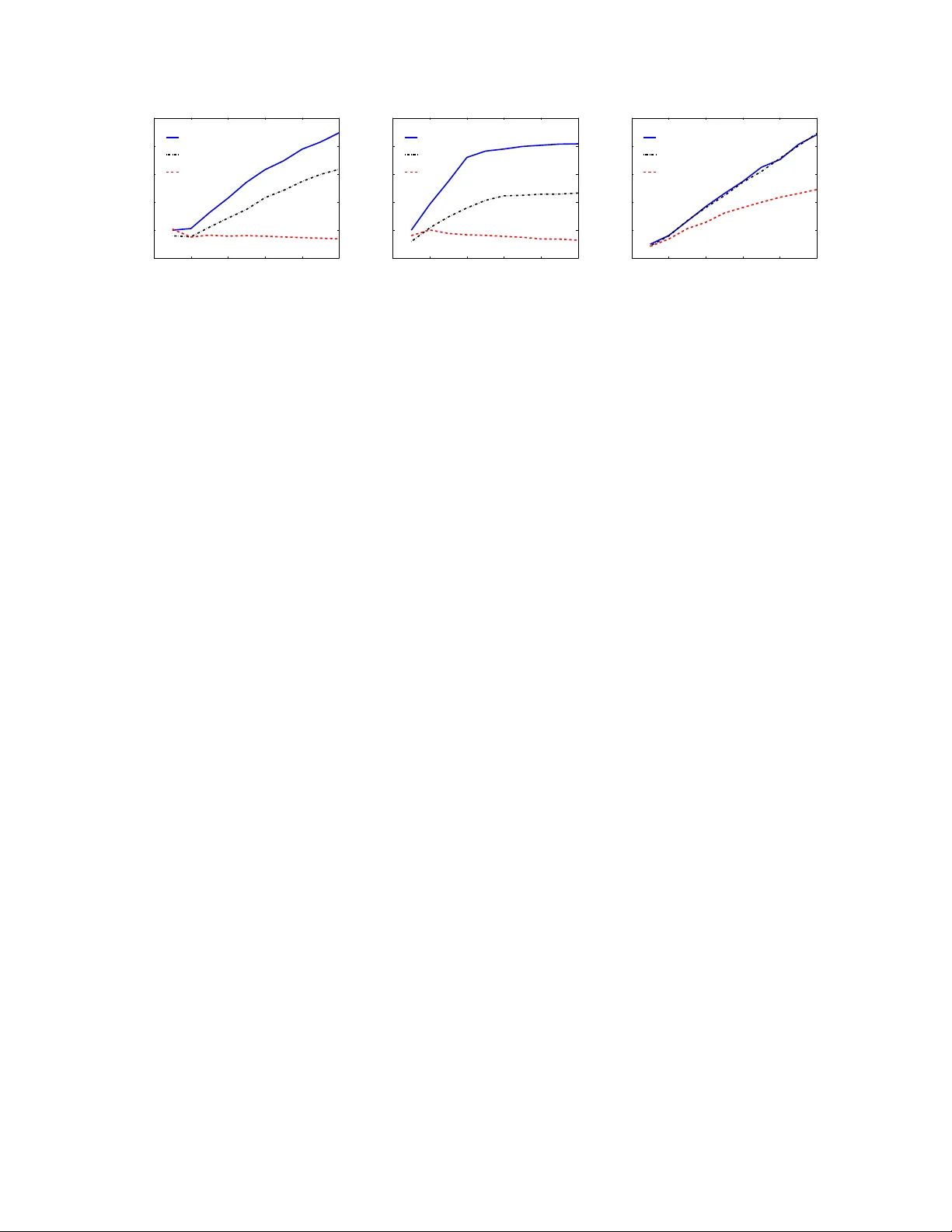
Hogwild! : A Lo c k-F ree Approac h to P arallelizing Sto c hastic Gradien t Descen t F eng Niu, Benjamin Rec ht, Christopher R ´ e and Stephen J. W righ t Computer Sciences Departmen t, Universit y of Wisconsin-Madison 1210 W Da yton St, Madison, WI 53706 June 2011 Abstract Sto c hastic Gradien t Descent (SGD) is a popular algorithm that can achiev e state-of-the-art p erformance on a v ariet y of machine learning tasks. Sev eral researc hers ha ve recently pro- p osed schemes to parallelize SGD, but all require p erformance-destro ying memory lo c king and sync hronization. This work aims to show using no vel theoretical analysis, algorithms, and im- plemen tation that SGD can b e implemented without any lo cking . W e presen t an up date sc heme called Hogwild! whic h allo ws processors access to shared memory with the possibility of o ver- writing each other’s w ork. W e sho w that when the asso ciated optimization problem is sp arse , meaning most gradien t updates only modify small parts of the decision v ariable, then Hogwild! ac hieves a nearly optimal rate of con vergence. W e demonstrate exp erimen tally that Hogwild! outp erforms alternativ e schemes that use lo c king b y an order of magnitude. Keyw ords. Incremen tal gradien t metho ds, Machine learning, Parallel computing, Multicore 1 In tro duction With its small memory fo otprin t, robustness against noise, and rapid learning rates, Stochastic Gra- dien t Descent (SGD) has prov ed to b e well suited to data-in tensive mac hine learning tasks [3, 5, 26]. Ho wev er, SGD’s scalability is limited by its inherently sequential nature; it is difficult to par- allelize. Nev ertheless, the recen t emergence of inexp ensiv e m ulticore pro cessors and mammoth, w eb-scale data sets has motiv ated researc hers to dev elop sev eral clev er parallelization sc hemes for SGD [4, 10, 12, 16, 30]. As man y large data sets are curren tly pre-pro cessed in a MapReduce-lik e parallel-pro cessing framework, m uch of the recent work on parallel SGD has fo cused naturally on MapReduce implementations. MapReduce is a p o werful to ol developed at Go ogle for extracting information from h uge logs (e.g., “find all the urls from a 100TB of W eb data”) that was designed to ensure fault tolerance and to simplify the main tenance and programming of large clusters of mac hines [9]. But MapReduce is not ideally suited for online, n umerically in tensive data analy- sis. Iterativ e computation is difficult to express in MapReduce, and the ov erhead to ensure fault tolerance can result in dismal throughput. Indeed, even Go ogle researchers themselves suggest that other systems, for example Dremel, are more appropriate than MapReduce for data analysis tasks [21]. F or some data sets, the sheer size of the data dictates that one use a cluster of machines. Ho w- ev er, there are a host of problems in which, after appropriate prepro cessing, the data necessary for 1 statistical analysis may consist of a few terab ytes or less. F or suc h problems, one can use a single inexp ensiv e work station as opp osed to a hundred thousand dollar cluster. Multicore systems hav e significan t p erformance adv antages, including (1) lo w latency and high throughput shared main memory (a pro cessor in suc h a system can write and read the shared physical memory at ov er 12GB/s with latency in the tens of nanoseconds); and (2) high bandwidth off multipl e disks (a thousand-dollar RAID can pump data into main memory at o v er 1GB/s). In con trast, a t ypical MapReduce setup will read incoming data at rates less than tens of MB/s due to frequen t c heck- p oin ting for fault tolerance. The high rates ac hiev able by multicore systems mo ve the bottlenecks in parallel computation to sync hronization (or locking) amongst the pro cessors [2, 13]. Thus, to enable scalable data analysis on a m ulticore mac hine, any p erforman t solution must minimize the o verhead of lo c king. In this work, we propose a simple strategy for eliminating the ov erhead asso ciated with lo c king: run SGD in p ar al lel without lo cks , a strategy that we call Hogwild! . In Hogwild! , pro cessors are allo wed equal access to shared memory and are able to up date individual comp onen ts of memory at will. Suc h a lo c k-free scheme might app ear do omed to fail as pro cessors could o verwrite each other’s progress. Ho wev er, when the data access is sp arse , meaning that individual SGD steps only mo dify a small part of the decision v ariable, we show that memory ov erwrites are rare and that they in tro duce barely any error into the computation when they do o ccur. W e demonstrate b oth theoretically and exp erimen tally a near linear sp eedup with the n umber of pro cessors on commonly o ccurring sparse learning problems. In Section 2, w e formalize a notion of sparsity that is sufficient to guarantee suc h a sp eedup and provide canonical examples of sparse machine learning problems in classification, collab orativ e filtering, and graph cuts. Our notion of sparsity allows us to pro vide theoretical guarantees of linear speedups in Section 4. As a by-product of our analysis, w e also deriv e rates of con vergence for algorithms with constant stepsizes. W e demonstrate that robust 1 /k conv ergence rates are p ossible with constant stepsize sc hemes that implemen t an exp onen tial back-off in the constant o ver time. This result is in teresting in of itself and sho ws that one need not settle for 1 / √ k rates to ensure robustness in SGD algorithms. In practice, we find that computational p erformance of a lo c k-free pro cedure exceeds ev en our theoretical guaran tees. W e exp erimen tally compare lo c k-free SGD to several recently prop osed metho ds. W e sho w that all metho ds that prop ose memory locking are significan tly slow er than their resp ectiv e lock-free coun terparts on a v ariet y of mac hine learning applications. 2 Sparse Separable Cost F unctions Our goal throughout is to minimize a function f : X ⊆ R n → R of the form f ( x ) = X e ∈ E f e ( x e ) . (2.1) Here e denotes a small subset of { 1 , . . . , n } and x e denotes the v alues of the vector x on the co ordinates indexed by e . The k ey observ ation that underlies our lo c k-free approach is that the natural cost functions associated with many mac hine learning problems of in terest are sp arse in the sense that | E | and n are b oth v ery large but each individual f e acts only on a very small n umber of comp onen ts of x . That is, each sub vector x e con tains just a few components of x . 2 (a) (b) (c) Figure 1: Example graphs induced by cost function. (a) A sparse SVM induces a h yp ergraph where each h yp eredge corresponds to one example. (b) A matrix completion example induces a bipartite graph b et ween the rows and columns with an edge b et w een t wo no des if an en try is rev ealed. (c) The induced hypergraph in a graph-cut problem is simply the graph whose cuts w e aim to find. The cost function (2.1) induces a hyp er gr aph G = ( V , E ) whose no des are the individual com- p onen ts of x . Each subv ector x e induces an edge in the graph e ∈ E consisting of some subset of no des. A few examples illustrate this concept. Sparse SVM. Supp ose our goal is to fit a supp ort vector mac hine to some data pairs E = { ( z 1 , y 1 ) , . . . , ( z | E | , y | E | ) } where z ∈ R n and y is a lab el for eac h ( z , y ) ∈ E . minimize x X α ∈ E max(1 − y α x T z α , 0) + λ k x k 2 2 , (2.2) and we know a priori that the examples z α are very sparse (see for example [14]). T o write this cost function in the form of (2.1), let e α denote the comp onen ts whic h are non-zero in z α and let d u denote the num b er of training examples whic h are non-zero in comp onen t u ( u = 1 , 2 , . . . , n ). Then we can rewrite (2.2) as minimize x X α ∈ E max(1 − y α x T z α , 0) + λ X u ∈ e α x 2 u d u ! . (2.3) Eac h term in the sum (2.3) dep ends only on the comp onen ts of x indexed b y the set e α . Matrix Completion. In the matrix completion problem, we are provided entries of a low-rank, n r × n c matrix Z from the index set E . Suc h problems arise in collab orativ e filtering, Euclidean distance estimation, and clustering [8, 17, 24]. Our goal is to reconstruct Z from this sparse sampling of data. A p opular heuristic recov ers the estimate of Z as a pro duct LR ∗ of factors obtained from the following minimization: minimize ( L , R ) X ( u,v ) ∈ E ( L u R ∗ v − Z uv ) 2 + µ 2 k L k 2 F + µ 2 k R k 2 F , (2.4) where L is n r × r , R is n c × r and L u (resp. R v ) denotes the u th (resp. v th) ro w of L (resp. R ) [17, 24, 27]. T o put this problem in sparse form, i.e., as (2.1), w e write (2.4) as minimize ( L , R ) X ( u,v ) ∈ E n ( L u R ∗ v − Z uv ) 2 + µ 2 | E u − | k L u k 2 F + µ 2 | E − v | k R v k 2 F o where E u − = { v : ( u, v ) ∈ E } and E − v = { u : ( u, v ) ∈ E } . 3 Graph Cuts. Problems inv olving minimum cuts in graphs frequen tly arise in mac hine learning (see [6] for a comprehensive survey). In suc h problems, we are giv en a sparse, nonnegative matrix W whic h indexes similarity b et ween entities. Our goal is to find a partition of the index set { 1 , . . . , n } that best conforms to this similarity matrix. Here the graph structure is explicitly determined b y the similarit y matrix W ; arcs corresp ond to nonzero entries in W . W e w ant to matc h each string to some list of D entities. Each node is asso ciated with a vector x i in the D -dimensional simplex S D = { ζ ∈ R D : ζ v ≥ 0 P D v =1 ζ v = 1 } . Here, tw o-wa y cuts use D = 2, but m ultiwa y-cuts with tens of thousands of classes also arise in entit y resolution problems [18]. F or example, we ma y hav e a list of n strings, and W uv migh t index the similarit y of each string. Several authors (e.g., [7]) prop ose to minimize the cost function minimize x X ( u,v ) ∈ E w uv k x u − x v k 1 sub ject to x v ∈ S D for v = 1 , . . . , n . (2.5) In all three of the preceding examples, the num b er of comp onen ts inv olv ed in a particular term f e is a small fraction of the total n umber of entries. W e formalize this notion by defining the follo wing statistics of the h yp ergraph G : Ω := max e ∈ E | e | , ∆ := max 1 ≤ v ≤ n |{ e ∈ E : v ∈ e }| | E | , ρ := max e ∈ E |{ ˆ e ∈ E : ˆ e ∩ e 6 = ∅}| | E | . (2.6) The quan tit y Ω simply quan tifies the size of the h yp er edges. ρ determines the maxim um fraction of edges that in tersect an y giv en edge. ∆ determines the maximum fraction of edges that in tersect an y v ariable. ρ is a measure of the sparsity of the h yp ergraph, while ∆ measures the no de-regularity . F or our examples, we can mak e the follo wing observ ations ab out ρ and ∆. 1. Sparse SVM . ∆ is simply the maximum frequency that any feature app ears in an example, while ρ measures ho w clustered the h yp ergraph is. If some features are v ery common across the data set, then ρ will b e close to one. 2. Matrix Completion . If w e assume that the pro vided examples are sampled uniformly at random and we see more than n c log( n c ) of them, then ∆ ≈ log( n r ) n r and ρ ≈ 2 log( n r ) n r . This follo ws from a c oup on c ol le ctor argumen t [8]. 3. Graph Cuts . ∆ is the maxim um degree divided b y | E | , and ρ is at most 2∆. W e no w describe a simple proto col that achiev es a linear sp eedup in the n um b er of pro cessors when Ω, ∆, and ρ are relativ ely small. 3 The Hogwild! Algorithm Here w e discuss the parallel pro cessing setup. W e assume a shared memory mo del with p pro ces- sors. The decision v ariable x is accessible to all pro cessors. Each pro cessor can read x , and can con tribute an up date vector to x . The vector x is stored in shared memory , and we assume that the comp onen twise addition op eration is atomic, that is x v ← x v + a 4 Algorithm 1 Hogwild! up date for individual pro cessors 1: lo op 2: Sample e uniformly at random from E 3: Read curren t state x e and ev aluate G e ( x ) 4: for v ∈ e do x v ← x v − γ b T v G e ( x ) 5: end lo op can b e p erformed atomically by any pro cessor for a scalar a and v ∈ { 1 , . . . , n } . This op eration do es not require a separate lo c king structure on most mo dern hardware: such an op eration is a single atomic instruction on GPUs and DSPs, and it can be implemented via a compare-and- exc hange op eration on a general purp ose multicore processor like the In tel Nehalem. In contrast, the op eration of updating man y comp onen ts at once requires an auxiliary lo c king structure. Eac h processor then follows the pro cedure in Algorithm 1. T o fully describ e the algorithm, let b v denote one of the standard basis elemen ts in R n , with v ranging from 1 , . . . , n . That is, b v is equal to 1 on the v th comp onen t and 0 otherwise. Let P v denote the Euclidean pro jection matrix on to the v th co ordinate, i.e., P v = b v b T v . P v is a diagonal matrix equal to 1 on the v th diagonal and zeros elsewhere. Let G e ( x ) ∈ R n denote a gradient or subgradient of the function f e m ultiplied b y | E | . That is, we extend f e from a function on the co ordinates of e to all of R n simply by ignoring the comp onen ts in ¬ e (i.e., not in e ). Then | E | − 1 G e ( x ) ∈ ∂ f e ( x ) . Here, G e is equal to zero on the comp onen ts in ¬ e . Using a sparse representation, we can calculate G e ( x ), only knowing the v alues of x in the components indexed b y e . Note that as a consequence of the uniform random sampling of e from E , we ha ve E [ G e ( x e )] ∈ ∂ f ( x ) . In Algorithm 1, eac h pro cessor samples an term e ∈ E uniformly at random, computes the gradien t of f e at x e , and then writes x v ← x v − γ b T v G e ( x ) , for each v ∈ e (3.1) Imp ortan tly , note that the pro cessor mo difies only the v ariables indexed b y e , lea ving all of the comp onen ts in ¬ e (i.e., not in e ) alone. W e assume that the stepsize γ is a fixed constan t. Ev en though the pro cessors ha ve no kno wledge as to whether an y of the other processors ha v e mo dified x , w e define x j to b e the state of the decision v ariable x after j up dates ha ve b een p erformed 1 . Since t wo pro cessors can write to x at the same time, we need to b e a bit careful with this definition, but w e simply break ties at random. Note that x j is generally up dated with a stale gradien t, which is based on a v alue of x read man y clock cycles earlier. W e use x k ( j ) to denote the v alue of the decision v ariable used to compute the gradient or subgradien t that yields the state x j . In what follows, w e provide conditions under whic h this async hronous, incremental gradien t algorithm con verges. Moreo ver, we sho w that if the h yp ergraph induced by f is isotropic and sparse, then this algorithm con verges in nearly the same num b er of gradient steps as its serial coun terpart. Since we are running in parallel and without lo c ks, this means that we get a nearly linear sp eedup in terms of the n um b er of processors. 1 Our notation ov erloads subscripts of x . F or clarity throughout, subscripts i, j , and k refer to iteration counts, and v and e refer to comp onen ts or subsets of comp onen ts. 5 4 F ast Rates for Lo ck-F ree P arallelism W e no w turn to our theoretical analysis of Hogwild! proto cols. T o mak e the analysis tractable, w e assume that w e up date with the follo wing “with replacemen t” pro cedure: each pro cessor samples an edge e uniformly at random and computes a subgradien t of f e at the curren t v alue of the decision v ariable. Then it c ho oses an v ∈ e uniformly at random and up dates x v ← x v − γ | e | b T v G e ( x ) Note that the stepsize is a factor | e | larger than the step in (3.1). Also note that this up date is completely equiv alent to x ← x − γ | e |P T v G e ( x ) . (4.1) This notation will b e more conv enient for the subsequen t analysis. This with replacement sc heme assumes that a gradient is computed and then only one of its comp onen ts is used to up date the decision v ariable. Suc h a sc heme is computationally wasteful as the rest of the comp onen ts of the gradient carry information for decreasing the cost. Consequently , in practice and in our experiments, we p erform a mo dification of this pro cedure. W e partition out the edges without r eplac ement to all of the pro cessors at the b eginning of each ep o c h. The pro cessors then perform ful l up dates of all of the components of eac h edge in their respective queues. How ever, w e emphasize again that we do not implement any locking mechanisms on an y of the v ariables. W e do not analyze this “without replacemen t” pro cedure b ecause no one has achiev ed tractable analyses for SGD in any without replacement sampling mo dels. Indeed, to our knowledge, all analysis of without-replacemen t sampling yields rates that are comparable to a standard subgradient descent algorithm whic h takes steps along the full gradien t of (2.1) (see, for example [22]). That is, these analyses suggest that without-replacement sampling should require a factor of | E | more steps than with-replacemen t sampling. In practice, this worst case b eha vior is nev er observed. In fact, it is con ven tional wisdom in machine learning that without-replacement sampling in sto c hastic gradient descen t actually outp erforms the with-replacement v ariants on whic h all of the analysis is based. T o state our theoretical results, we m ust describ e sev eral quan tities that imp ortan t in the analysis of our parallel stochastic gradien t descen t sc heme. W e follo w the notation and assumptions of Nemirovski et al [23]. T o simplify the analysis, w e will assume that eac h f e in (2.1) is a con v ex function. W e assume Lipsc hitz contin uous differen tiability of f with Lipsc hitz constant L : k∇ f ( x 0 ) − ∇ f ( x ) k ≤ L k x 0 − x k , ∀ x 0 , x ∈ X . (4.2) W e also assume f is strongly conv ex with modulus c . By this we mean that f ( x 0 ) ≥ f ( x ) + ( x 0 − x ) T ∇ f ( x ) + c 2 k x 0 − x k 2 , for all x 0 , x ∈ X . (4.3) When f is strongly conv ex, there exists a unique minimizer x ? and w e denote f ? = f ( x ? ). W e additionally assume that there exists a constan t M such that k G e ( x e ) k 2 ≤ M almost surely for all x ∈ X . (4.4) W e assume throughout that γ c < 1. (Indeed, when γ c > 1, ev en the ordinary gradient descent algorithms will div erge.) Our main results are summarized b y the follo wing 6 Prop osition 4.1 Supp ose in A lgorithm 1 that the lag b etwe en when a gr adient is c ompute d and when it is use d in step j — namely, j − k ( j ) — is always less than or e qual to τ , and γ is define d to b e γ = ϑc 2 LM 2 Ω  1 + 6 ρτ + 4 τ 2 Ω∆ 1 / 2  . (4.5) for some  > 0 and ϑ ∈ (0 , 1) . Define D 0 := k x 0 − x ? k 2 and let k b e an inte ger satisfying k ≥ 2 LM 2 Ω  1 + 6 τ ρ + 6 τ 2 Ω∆ 1 / 2  log( LD 0 / ) c 2 ϑ . (4.6) Then after k c omp onent up dates of x , we have E [ f ( x k ) − f ? ] ≤  . In the case that τ = 0, this reduces to precisely the rate ac hieved by the serial SGD proto col. A similar rate is achiev ed if τ = o ( n 1 / 4 ) as ρ and ∆ are typically b oth o (1 /n ). In our setting, τ is proportional to the num b er of pro cessors, and hence as long as the n um b er of pro cessors is less n 1 / 4 , we get nearly the same recursion as in the linear rate. W e pro ve Prop osition 4.1 in t wo steps in the App endix. First, we demonstrate that the sequence a j = 1 2 E [ k x j − x ? k 2 ] satisfies a recursion of the form a j ≤ (1 − c r γ )( a j +1 − a ∞ ) + a ∞ for some constan t a ∞ that dep ends on many of the algorithm parameters but not on the state, and some constan t c r < c . This c r is an “effective curv ature” for the problem which is smaller that the true curv ature c b ecause of the errors in tro duced b y our up date rule. Using the fact that c r γ < 1, we will show in Section 5 how to determine an upp er b ound on k for which a k ≤ /L . Proposition 4.1 then follows b ecause E [ f ( x k ) − f ( x ? )] ≤ La k since the gradient of f is Lipschitz. A full pro of is pro vided in the app endix. Note that up to the log (1 / ) term in (4.6), our analysis nearly provides a 1 /k rate of con v ergence for a constant stepsize SGD scheme, b oth in the serial and parallel cases. Moreov er, note that our rate of conv ergence is fairly robust to error in the v alue of c ; we pay linearly for our underestimate of the curv ature of f . In contrast, Nemirovski et al demonstrate that when the stepsize is inv ersely prop ortional to the iteration counter, an ov erestimate of c can result in exp onential slo w-do wn [23]! W e no w turn to demonstrating that w e can eliminate the log term from (4.6) by a slightly more complicated proto col where the stepsize is slo wly decreased after a large n um b er of iterations. 5 Robust 1 /k rates. Supp ose we run Algorithm 1 for a fixed n umber of gradien t up dates K with stepsize γ < 1 /c . Then, w e w ait for the threads to coalesce, reduce γ by a constant factor β ∈ (0 , 1), and run for β − 1 K iterations. In some sense, this piecewise constant stepsize proto col approximates a 1 /k diminishing stepsize. The main difference with the following analysis from previous work is that our stepsizes are alwa ys less than 1 /c in contrast to b eginning with very large stepsizes. Alwa ys working with small stepsizes allows us to a void the p ossible exp onential slow-do wns that o ccur with standard diminishing stepsize sc hemes. T o b e precise, suppose a k is any sequence of real n umbers satisfying a k +1 ≤ (1 − c r γ )( a k − a ∞ ( γ )) + a ∞ ( γ ) (5.1) where a ∞ is some non-negativ e function of γ satisfying a ∞ ( γ ) ≤ γ B 7 and c r and B are constan ts. This recursion underlies many conv ergence pro ofs for SGD where a k denotes the distance to the optimal solution after k iterations. W e will deriv e appropriate constan ts for Hogwild! in the App endix. W e will also discuss below what these constan ts are for standard sto c hastic gradient descent algorithms. F actoring out the dep endence on γ will b e useful in what follows. Unwrapping (5.1) we ha ve a k ≤ (1 − c r γ ) k ( a 0 − a ∞ ( γ )) + a ∞ ( γ ) . Supp ose w e w ant this quantit y to b e less than  . It is sufficien t that b oth terms are less than / 2. F or the second term, this means that it is sufficient to set γ ≤  2 B . (5.2) F or the first term, we then need (1 − γ c r ) k a 0 ≤ / 2 whic h holds if k ≥ log(2 a 0 / ) γ c r . (5.3) By (5.2), w e should pic k γ = ϑ 2 B for ϑ ∈ (0 , 1]. Combining this with (5.3) tells us that after k ≥ 2 B log(2 a 0 / ) ϑc r iterations w e will ha v e a k ≤  . This righ t off the bat almost gives us a 1 /k rate, mo dulo the log(1 / ) factor. T o eliminate the log factor, we can implemen t a back off scheme where w e reduce the stepsize by a constant factor after sev eral iterations. This back off scheme will ha ve tw o phases: the first phase will consist of con verging to the ball ab out x ? of squared radius less than 2 B c r at an exp onen tial rate. Then we will con v erge to x ? b y shrinking the stepsize. T o calculate the n um b er of iterates required to get inside a ball of squared radius 2 B c r , supp ose the initial stepsize is chosen as γ = ϑ c r (0 < ϑ < 1). This choice of stepsize guarantees that the a k con verge to a ∞ . W e use the parameter ϑ to demonstrate that we do not suffer m uch for underestimating the optimal stepsize (i.e., ϑ = 1) in our algorithms. Using (5.3) w e find that k ≥ ϑ − 1 log  a 0 c r ϑB  (5.4) iterations are sufficien t to con v erge to this ball. Note that this is a linear rate of con vergence. No w assume that a 0 < 2 ϑB c r . Let’s reduce the stepsize b y a factor of β eac h ep o c h. This reduces the achiev ed  b y a factor of β . Th us, after log β ( a 0 / ) ep o c hs, we will b e at accuracy  . The total n umber of iterations required is then the sum of terms with the form (5.3), with a 0 set to b e the radius achiev ed b y the previous ep och and  set to b e β times this a 0 . Hence, for ep o c h n umber ν , the initial distance is β ν − 1 a 0 and the final radius is β ν . Summing ov er all of the ep o c hs (except for 8 the initial phase) giv es log β ( a 0 / ) X k =1 log(2 /β ) ϑβ k = log(2 /β ) ϑ log β ( a 0 / ) X k =1 β − k = log(2 /β ) ϑ β − 1 ( a 0 / ) − 1 β − 1 − 1 ≤ a 0 ϑ log(2 /β ) 1 − β ≤ 2 B c r  log(2 /β ) 1 − β . (5.5) This expression is minimized by selecting a bac koff parameter ≈ 0 . 37. Also, note that when we reduce the stepsize b y β , we need to run for β − 1 more iterations. Com bining (5.4) and (5.5), w e estimate a total num b er of iterations equal to k ≥ ϑ − 1 log  a 0 c r ϑB  + 2 B c r  log(2 /β ) 1 − β are sufficient to guaran tee that a k ≤  . Rearranging terms, the following tw o expressions give  in terms of all of the algorithm param- eters:  ≤ 2 log (2 /β ) 1 − β · B c r · 1 k − ϑ − 1 log  a 0 c r ϑB  . (5.6) 5.1 Consequences for serial SGD Let us compare the results of this constan t step-size proto col to one where the stepsize at iteration k is set to b e γ 0 /k for some initial step size γ for the standard (serial) incremental gradien t algorithm applied to (2.1). Nemiro vski et al [23] show that the expected squared distance to the optimal solution, a k , satisfies a k +1 ≤ (1 − 2 cγ k ) a k + 1 2 γ 2 k M 2 . W e can put this recursion in the form (5.1) by setting γ k = γ , c r = 2 c , B = M 2 4 c , and a ∞ = γ M 2 4 c . The authors of [23] demonstrate that a large step size: γ k = Θ 2 ck with Θ > 1 yields a b ound a k ≤ 1 k max  M 2 c 2 · Θ 2 4Θ − 4 , D 0  On the other hand, a constan t step size proto col ac hieves a k ≤ log(2 /β ) 4(1 − β ) · M 2 c 2 · 1 k − ϑ − 1 log  4 D 0 c 2 ϑM 2  . This b ound is obtained b y plugging the algorithm parameters in to (5.6) and letting D 0 = 2 a 0 . Note that b oth b ounds hav e asymptotically the same dep endence on M , c , and k . The expres- sion log(2 /β ) 4(1 − β ) 9 is minimized when β ≈ 0 . 37 and is equal to 1 . 34. The expression Θ 2 4Θ − 4 is minimized when Θ = 2 and is equal to 1 at this minimum. So the leading constant is slightly w orse in the constan t stepsize proto col when all of the parameters are set optimally . Ho wev er, if D 0 ≥ M 2 /c 2 , the 1 /k proto col has error prop ortional to D 0 , but our constant stepsize proto col still has only a logarithmic dep endence on the initial distance. Moreov er, the constan t stepsize scheme is m uch more robust to o verestimates of the curv ature parameter c . F or the 1 /k proto cols, if one o verestimates the curv ature (corresponding to a small v alue of Θ), one can get arbitrarily slow rates of con vergence. An simple, one dimensional example in [23] shows that Θ = 0 . 2 can yield a con vergence rate of k − 1 / 5 . In our sc heme, ϑ = 0 . 2 simply increases the n umber of iterations b y a factor of 5. The prop osed fix in [23] for the sensitivit y to curv ature estimates results in asymptotically slo wer conv ergence rates of 1 / √ k . It is important to note that we need not settle for these slow er rates and can still achiev e robust conv ergence at 1 /k rates. 5.2 P arallel Implemen tation of a Back off Sc heme The scheme describ ed ab out results in a 1 /k rate of con vergence for Hogwild! with the only sync hronization ov erhead o ccurring at the end of each “round” or “ep o c h” of iteration. When implemen ting a back off scheme for Hogwild! , the pro cessors hav e to agree on when to reduce the stepsize. One simple scheme for this is to run all of the pro cessors for a fixed num b er of iterations, w ait for all of the threads to complete, and then globally reduce the stepsize in a master thread. W e note that one can eliminate the need for the threads to coalesce by sending out-of-band messages to the pro cessors to signal when to reduce γ . This complicates the theoretical analysis as there ma y b e times when different pro cessors are running with differen t stepsizes, but in practice could allo w one to av oid synchronization costs. W e do not implemen t this scheme, and so do not analyze this idea further. 6 Related W ork Most schemes for parallelizing sto c hastic gradien t descent are v ariants of ideas presen ted in the seminal text b y Bertsek as and Tsitsiklis [4]. F or instance, in this text, they describ e using stale gradien t updates computed across man y computers in a master-w orker setting and describ e settings where different pro cessors control access to particular comp onents of the decision v ariable. They pro ve global con vergence of these approaches, but do not pro vide rates of con vergence (This is one w ay in which our w ork extends this prior researc h). These authors also sho w that SGD con v ergence is robust to a v ariety of mo dels of dela y in computation and communication in [29]. W e also note that constant stepsize proto cols with bac koff pro cedures are canonical in SGD practice, but p erhaps not in theory . Some theoretical work whic h has at least demonstrated con- v ergence of these proto cols can b e found in [20, 28]. These w orks do not establish the 1 /k rates whic h w e provided ab o ve. Recen tly , a v ariety of parallel sc hemes hav e been proposed in a v ariety of contexts. In MapRe- duce settings, Zinkevic h et al prop osed running man y instances of sto c hastic gradien t descen t on 10 Hogwild! R ound R obin t yp e data size ρ ∆ time train tes t time train test set (GB) (s) error error (s) error error SVM R CV1 0.9 0.44 1.0 9.5 0.297 0.339 61.8 0.297 0.339 MC Netflix 1.5 2.5e-3 2.3e-3 301.0 0.754 0.928 2569.1 0.754 0.927 KDD 3.9 3.0e-3 1.8e-3 877.5 19.5 22.6 7139.0 19.5 22.6 Jum b o 30 2.6e-7 1.4e-7 9453.5 0.031 0.013 N/A N/A N/A Cuts DBLife 3e-3 8.6e-3 4.3e-3 230.0 10.6 N/A 413.5 10.5 N/A Ab domen 18 9.2e-4 9.2e-4 1181.4 3.99 N/A 7467.25 3.99 N/A Figure 2: Comparison of wall clo c k time across of Hogwild! and RR. Each algorithm is run for 20 ep o c hs and parallelized ov er 10 cores. differen t mac hines and a veraging their output [30]. Though the authors claim this metho d can reduce b oth the v ariance of their estimate and the o verall bias, w e sho w in our exp erimen ts that for the sorts of problems we are concerned with, this metho d do es not outp erform a serial scheme. Sc hemes inv olving the av eraging of gradients via a distributed proto col ha v e also b een prop osed b y several authors [10, 12]. While these metho ds do achiev e linear sp eedups, they are difficult to implement efficiently on m ulticore machines as they require massive comm unication ov erhead. Distributed av eraging of gradients requires message passing b et ween the cores, and the cores need to synchronize frequently in order to compute reasonable gradien t av erages. The w ork most closely related to our o wn is a round-robin sc heme prop osed b y Langford et al [16]. In this sc heme, the processors are ordered and each up date the decision v ariable in order. When the time required to lo c k memory for writing is dw arfed b y the gradien t computation time, this metho d results in a linear sp eedup, as the errors induced by the lag in the gradients are not to o sev ere. How ever, we note that in man y applications of in terest in machine learning, gradien t computation time is incredibly fast, and w e no w demonstrate that in a v ariety of applications, Hogwild! outperforms suc h a round-robin approach by an order of magnitude. 7 Exp erimen ts W e ran numerical exp erimen ts on a v ariety of mac hine learning tasks, and compared against a round-robin approach proposed in [16] and implemented in V owpal W abbit [15]. W e refer to this approac h as RR. T o b e as fair as p ossible to prior art, we hand co ded RR to b e nearly identical to the Hogwild! approach, with the only difference being the sc hedule for how the gradien ts are up dated. One notable change in RR from the V owpal W abbit softw are release is that we optimized RR’s locking and signaling mec hanisms to use spinlocks and busy w aits (there is no need for generic signaling to implemen t round robin). W e v erified that this optimization results in nearly an order of magnitude increase in wall clo c k time for all problems that w e discuss. W e also compare against a mo del which we call AIG whic h can b e seen as a middle ground b et w een RR and Hogwild! . AIG runs a proto col iden tical to Hogwild! except that it lo c ks all of the v ariables in e in b efore and after the for lo op on line 4 of Algorithm 1. Our exp erimen ts demonstrate that ev en this fine-grained lo c king induces undesirable slo w-downs. All of the exp erimen ts w ere co ded in C++ are run on an identical configuration: a dual Xeon X650 CPUs (6 cores each x 2 h yp erthreading) machine with 24GB of RAM and a softw are RAID-0 11 0 2 4 6 8 10 0 1 2 3 4 5 Number of Splits Speedup (a) Hogwild AIG RR 0 2 4 6 8 10 0 1 2 3 4 5 Number of Splits Speedup (b) Hogwild AIG RR 0 2 4 6 8 10 0 2 4 6 8 10 Number of Splits Speedup (c) Hogwild AIG RR Figure 3: T otal CPU time versus n umber of threads for (a) RCV1, (b) Ab domen, and (c) DBLife. o ver 7 2TB Seagate Constellation 7200RPM disks. The k ernel is Linux 2.6.18-128. W e never use more than 2GB of memory . All training data is stored on a seven-disk raid 0. W e implemen ted a custom file scanner to demonstrate the speed of reading data sets of disk into small shared memory . This allows us to read data from the raid at a rate of nearly 1GB/s. All of the exp erimen ts use a constant stepsize γ which is diminished by a factor β at the end of eac h pass o ver the training set. W e run all exp erimen ts for 20 such passes, even though less ep o c hs are often sufficien t for conv ergence. W e show results for the largest v alue of the learning rate γ whic h conv erges and w e use β = 0 . 9 throughout. W e note that the results lo ok the same across a large range of ( γ , β ) pairs and that all three parallelization sc hemes ac hieve train and test errors within a few percent of one another. W e presen t exp erimen ts on the classes of problems described in Section 2. Sparse SVM. W e tested our sparse SVM implementation on the Reuters RCV1 data set on the binary text classification task CCA T [19]. There are 804,414 examples split in to 23,149 training and 781,265 test examples, and there are 47,236 features. W e swapped the training set and the test set for our exp erimen ts to demonstrate the scalability of the parallel multicore algorithms. In this example, ρ = 0 . 44 and ∆ = 1 . 0—large v alues that suggest a bad case for Hogwild! . Nev ertheless, in Figure 3(a), we see that Hogwild! is able to ac hieve a factor of 3 sp eedup with while RR gets worse as more threads are added. Indeed, for fast gradients, RR is w orse than a serial implementation. F or this data set, we also implemen ted the approach in [30] whic h runs m ultiple SGD runs in parallel and av erages their output. In Figure 5(b), we display at the train error of the ensemble a verage across parallel threads at the end of each pass ov er the data. W e note that the threads only communicate at the v ery end of the computation, but we wan t to demonstrate the effect of parallelization on train error. Eac h of the parallel threads touches ev ery data example in each pass. Th us, the 10 thread run do es 10x more gradient computations than the serial version. Here, the error is the same whether we run in serial or with ten instances. W e conclude that on this problem, there is no adv antage to running in parallel with this av eraging scheme. Matrix Completion. W e ran Hogwild! on three very large matrix completion problems. The Netflix Prize data set has 17,770 rows, 480,189 columns, and 100,198,805 revealed en tries. The KDD Cup 2011 (task 2) data set has 624,961 ro ws, 1,000,990, columns and 252,800,275 revealed en tries. W e also syn thesized a low-rank matrix with rank 10, 1e7 rows and columns, and 2e9 rev ealed en tries. W e refer to this instance as “Jumbo.” In this syn thetic example, ρ and ∆ are b oth around 1e-7. These v alues con trast sharply with the real data sets where ρ and ∆ are b oth 12 0 2 4 6 8 10 0 1 2 3 4 5 6 Number of Splits Speedup (a) Hogwild AIG RR 0 2 4 6 8 10 0 1 2 3 4 5 6 Number of Splits Speedup (b) Hogwild AIG RR 0 2 4 6 8 10 0 2 4 6 8 Number of Splits Speedup (c) Hogwild AIG Figure 4: T otal CPU time versus n umber of threads for the matrix completion problems (a) Netflix Prize, (b) KDD Cup 2011, and (c) the syn thetic Jum b o exp erimen t. on the order of 1e-3. Figure 5(a) sho ws the sp eedups for these three data sets using Hogwild! . Note that the Jum b o and KDD examples do not fit in our allotted memory , but even when reading data off disk, Hogwild! attains a near linear sp eedup. The Jum b o problem takes just ov er tw o and a half hours to complete. Sp eedup graphs comparing Hogwild! to AIG and RR on the three matrix completion exp erimen ts are provided in Figure 4. Similar to the other exp erimen ts with quickly computable gradients, RR do es not sho w an y improv ement o ver a serial approac h. In fact, with 10 threads, RR is 12% slow er than serial on KDD Cup and 62% slow er on Netflix. In fact, it is to o slo w to complete the Jum b o exp eriment in any reasonable amount of time, while the 10-wa y parallel Hogwild! implementation solves this problem in under three hours. Graph Cuts. Our first cut problem w as a standard image segmen tation by graph cuts problem p opular in computer vision. W e computed a t wo-w ay cut of the abdomen data set [1]. This data set consists of a v olumetric scan of a human abdomen, and the goal is to segmen t the image into organs. The image has 512 × 512 × 551 v oxels, and the asso ciated graph is 6-connected with maxim um capacity 10. Both ρ and ∆ are equal to 9.2e-4 W e see that Hogwild! sp eeds up the cut problem by more than a factor of 4 with 10 threads, while RR is twice as slow as the serial version. Our second graph cut problem sought a mulit-w ay cut to determine en tity recognition in a large database of w eb data. W e created a data set of clean entit y lists from the DBLife w ebsite and of en tity men tions from the DBLife W eb Crawl [11]. The data set consists of 18,167 entities and 180,110 mentions and similarities given by string similarit y . In this problem eac h sto c hastic gradien t step must compute a Euclidean pro jection on to a simplex of dimension 18,167. As a result, the individual sto c hastic gradien t steps are quite slow. Nonetheless, the problem is still v ery sparse with ρ =8.6e-3 and ∆=4.2e-3. Consequently , in Figure 3, w e see the that Hogwild! ac hieves a ninefold speedup with 10 cores. Since the gradients are slo w, RR is able to achiev e a parallel sp eedup for this problem, ho wev er the sp eedup with ten pro cessors is only by a factor of 5. That is, ev en in this case where the gradient computations are very slow, Hogwild! outp erforms a round-robin sc heme. What if the gradients are slow? As w e saw with the DBLIFE data set, the RR metho d do es get a nearly linear sp eedup when the gradien t computation is slow. This raises the question whether RR ev er outperforms Hogwild! for slo w gradien ts. T o answer this question, w e ran the R CV1 exp erimen t again and introduced an artificial delay at the end of each gradien t computation to simulate a slo w gradient. In Figure 5(c), we plot the wall clo c k time required to solv e the SVM problem as w e v ary the dela y for both the RR and Hogwild! approaches. 13 0 2 4 6 8 10 0 2 4 6 8 Number of Splits Speedup (a) Jumbo Netflix KDD 0 5 10 15 20 0.31 0.315 0.32 0.325 0.33 0.335 0.34 Epoch Train Error (b) 1 Thread 3 Threads 10 Threads 10 0 10 2 10 4 10 6 0 2 4 6 8 10 Gradient Delay (ns) Speedup (c) Hogwild AIG RR Figure 5: (a) Sp eedup for the three matrix completion problems with Hogwild! . In all three cases, massiv e speedup is achiev ed via parallelism. (b) The training error at the end of each ep och of SVM training on R CV1 for the av eraging algorithm [30]. (c) Sp eedup ac hieved ov er serial metho d for v arious levels of dela ys (measured in nanoseconds). Notice that Hogwild! ac hieves a greater decrease in computation time across the b oard. The sp eedups for b oth metho ds are the same when the dela y is few milliseconds. That is, if a gradien t tak es longer than one millisecond to compute, RR is on par with Hogwild! (but not b etter). A t this rate, one is only able to compute ab out a million sto c hastic gradients p er hour, so the gradient computations must b e very lab or intensiv e in order for the RR metho d to be competitive. 8 Conclusions Our prop osed Hogwild! algorithm takes adv an tage of sparsity in machine learning problems to enable near linear speedups on a v ariety of applications. Empirically , our implementations outp erform our theoretical analysis. F or instance, ρ is quite large in the R CV1 SVM problem, y et w e still obtain significan t speedups. Moreo ver, our algorithms allow parallel speedup ev en when the gradients are computationally intensiv e. Our Hogwild! sc hemes can b e generalized to problems where some of the v ariables o ccur quite frequen tly as well. W e could c ho ose to not up date certain v ariables that w ould b e in particularly high con ten tion. F or instance, we might wan t to add a bias term to our Support V ector Mac hine, and we could still run a Hogwild! sc heme, up dating the bias only every thousand iterations or so. F or future work, it would b e of in terest to enumerate structures that allo w for parallel gradien t computations with no collisions at all. That is, it may b e p ossible to bias the SGD iterations to completely av oid memory conten tion b et ween pro cessors. F or example, recent w ork proposed a biased ordering of the sto c hastic gradien ts in matrix completion problems that completely av oids memory conten tion b et ween pro cessors [25]. An in vestigation in to how to generalize this approac h to other structures and problems would enable ev en faster computation of machine learning problems. Ac kno wledgemen ts BR is generously supp orted by ONR a ward N00014-11-1-0723 and NSF aw ard CCF-1139953. CR is generously supp orted by the Air F orce Research Lab oratory (AFRL) under prime con tract no. F A8750-09-C-0181, the NSF CAREER aw ard under I IS-1054009, ONR aw ard N000141210041, and gifts or researc h aw ards from Google, LogicBlox, and Johnson Controls, Inc. SJW is generously 14 supp orted by NSF aw ards DMS-0914524 and DMS-0906818 and DOE aw ard DE-SC0002283. An y opinions, findings, and conclusion or recommendations expressed in this work are those of the authors and do not necessarily reflect the views of any of the ab o ve sp onsors including D ARP A, AFRL, or the US gov ernment. References [1] Max-flo w problem instances in vision. F rom http://vision.csd.uwo.ca/data/maxflow/ . [2] K. Asano vic and et al . The landscap e of parallel computing research: A view from b erk eley . T echnical Rep ort UCB /EECS-2006-183, Electrical Engineering and Computer Sciences, Universit y of California at Berkeley , 2006. [3] D. P . Bertsek as. Nonline ar Pr o gr amming . A thena Scien tific, Belmon t, MA, 2nd edition, 1999. [4] D. P . Bertsek as and J. N. Tsitsiklis. Par al lel and Distribute d Computation: Numeric al Metho ds . Athena Scien tific, Belmon t, MA, 1997. [5] L. Bottou and O. Bousquet. The tradeoffs of large scale learning. In A dvanc es in Neur al Information Pr o c essing Systems , 2008. [6] Y. Bo yko v and V. Kolmogorov. An exp erimen tal comparison of min-cut/max-flo w algorithms for energy minimization in vision. IEEE T r ansactions on Pattern Analysis and Machine Intel ligenc e , 26(9):1124– 1137, 2004. [7] G. C˘ alinescu, H. Karloff, and Y. Rabani. An improv ed approximation algorithm for multiw ay cut. In Pr o c e e dings of the thirtieth annual A CM Symp osium on The ory of Computing , pages 48–52, 1998. [8] E. Cand` es and B. Rech t. Exact matrix completion via conv ex optimization. F oundations of Computa- tional Mathematics , 9(6):717–772, 2009. [9] J. Dean and S. Ghemaw at. MapReduce: simplified data pro cessing on large clusters. Communic ations of the ACM , 51(1):107–113, 2008. [10] O. Dekel, R. Gilad-Bac hrach, O. Shamir, and L. Xiao. Optimal distributed online prediction using mini-batc hes. T echnical rep ort, Microsoft Researc h, 2011. [11] A. Doan. http://dblife.cs.wisc.edu . [12] J. Duchi, A. Agarwal, and M. J. W ainwrigh t. Distributed dual av eraging in netw orks. In A dvanc es in Neur al Information Pr o c essing Systems , 2010. [13] S. H. F uller and L. I. Millett, editors. The F utur e of Computing Performanc e: Game Over or Next L evel . Committee on Sustaining Gro wth in Computing P erformance. The National Academies Press, W ashington, D.C., 2011. [14] T. Joachims. T raining linear svms in linear time. In Pr o c e e dings of the ACM Confer enc e on Know le dge Disc overy and Data Mining (KDD) , 2006. [15] J. Langford. https://github.com/JohnLangford/vowpal_wabbit/wiki . [16] J. Langford, A. J. Smola, and M. Zinkevic h. Slow learners are fast. In A dvanc es in Neur al Information Pr o c essing Systems , 2009. [17] J. Lee, , B. Rech t, N. Srebro, R. R. Salakhutdino v, and J. A. T ropp. Practical large-scale optimization for max-norm regularization. In A dvanc es in Neur al Information Pr o c essing Systems , 2010. [18] T. Lee, Z. W ang, H. W ang, and S. Hwang. W eb scale entit y resolution using relational evidence. T echnical rep ort, Microsoft Researc h, 2011. Av ailable at http://research.microsoft.com/apps/ pubs/default.aspx?id=145839 . 15 [19] D. Lewis, Y. Y ang, T. Rose, and F. Li. RCV1: A new b enc hmark collection for text categorization researc h. Journal of Machine L e arning R ese ar ch , 5:361–397, 2004. [20] Z. Q. Luo and P . Tseng. Analysis of an approximate gradient pro jection metho d with applications to the backpropagation algorithm. Optimization Metho ds and Softwar e , 4:85–101, 1994. [21] S. Melnik, A. Gubarev, J. J. Long, G. Romer, S. Shiv akumar, M. T olton, and T. V assilakis. Dremel: In teractive analysis of web-scale datasets. In Pr o c e e dings of VLDB , 2010. [22] A. Nedic and D. P . Bertsek as. Con vergence rate of incremental subgradient algorithms. In S. Uryasev and P . M. Pardalos, editors, Sto chastic Optimization: Algorithms and Applic ations , pages 263–304. Klu wer Academic Publishers, 2000. [23] A. Nemirovski, A. Juditsky , G. Lan, and A. Shapiro. Robust sto c hastic approximation approach to sto c hastic programming. SIAM Journal on Optimization , 19(4):1574–1609, 2009. [24] B. Rec ht, M. F azel, and P . Parrilo. Guaranteed minim um rank solutions of matrix equations via nuclear norm minimization. SIAM R eview , 52(3):471–501, 2010. [25] B. Rec ht and C. R´ e. Parallel stochastic gradien t algorithms for large-scale matrix completion. Submitted for publication. Preprin t a v ailable at http://pages.cs.wisc.edu/ ~ brecht/publications.html , 2011. [26] S. Shalev-Shw artz and N. Srebro. SVM Optimization: Inv erse dependence on training set size. In Pr o c e e dings of the 25th Internation Confer enc e on Machine L e arning , 2008. [27] N. Srebro, J. Rennie, and T. Jaakk ola. Maxim um margin matrix factorization. In A dvanc es in Neur al Information Pr o c essing Systems , 2004. [28] P . Tseng. An incremental gradien t(-pro jection) metho d with momentum term and adaptive stepsize rule. SIAM Jour al on Optimization , 8(2):506–531, 1998. [29] J. Tsitsiklis, D. P . Bertsek as, and M. A thans. Distributed asynchronous deterministic and stochastic gradien t optimization algorithms. IEEE T r ansactions on A utomatic Contr ol , 31(9):803–812, 1986. [30] M. Zinkevic h, M. W eimer, A. Smola, and L. Li. Parallelized sto c hastic gradien t descent. A dvanc es in Neur al Information Pr o c essing Systems , 2010. A Analysis of Hogwild! It follows by rearrangement of (4.3) that ( x − x 0 ) T ∇ f ( x ) ≥ f ( x ) − f ( x 0 ) + 1 2 c k x − x 0 k 2 , for all x ∈ X . (A.1) In particular, b y setting x 0 = x ? (the minimizer) w e hav e ( x − x ? ) T ∇ f ( x ) ≥ 1 2 c k x − x ? k 2 , for all x ∈ X . (A.2) W e will mak e use of these identities frequently in what follo ws. 16 A.1 Dev eloping the recursion F or 1 ≤ v ≤ n , let P v denote the pro jection on to the v th comp onen t of R n . ( P v is a diagonal matrix with a 1 in the v th diagonal p osition and zeros elsewhere.) Similarly , for e ∈ E , w e let P e denote the pro jection onto the comp onents indexed by e — a diagonal matrix with ones in the p ositions indexed by e and zeros elsewhere. W e start with the update form ula (4.1). Recall that k ( j ) is the state of the decision v ariable’s coun ter when the up date to x j w as read. W e ha ve x j +1 = x j − γ | e j |P v j G e j ( x k ( j ) ) . By subtracting x ? from b oth sides, taking norms, we hav e 1 2 k x j +1 − x ? k 2 2 = 1 2 k x j − x ? k 2 2 − γ | e j | ( x j − x ? ) T P v j G e j ( x k ( j ) ) + 1 2 γ 2 | e j | 2 kP v j G e j ( x k ( j ) ) k 2 = 1 2 k x j − x ? k 2 2 − γ | e j | ( x j − x k ( j ) ) T P v j G e j ( x j ) − γ | e j | ( x j − x k ( j ) ) T P v j ( G e j ( x k ( j ) ) − G e j ( x j )) − γ | e j | ( x k ( j ) − x ? ) T P v j G e j ( x k ( j ) ) + 1 2 γ 2 | e j | 2 kP v j G e j ( x k ( j ) ) k 2 Let a j = 1 2 E [ k x j − x ? k 2 2 ]. By taking exp ectations of both sides and using the b ound (4.4), we obtain a j +1 ≤ a j − γ E [( x j − x k ( j ) ) T G e j ( x j )] − γ E [( x j − x k ( j ) ) T ( G e j ( x k ( j ) ) − G e j ( x j ))] − γ E [( x k ( j ) − x ? ) T G e j ( x k ( j ) )] + 1 2 γ 2 Ω M 2 . (A.3) where w e recall that Ω = max e ∈ E | e | . Here, in several places, we used the useful identit y: for any function ζ of x 1 , . . . , x j and any i ≤ j , we hav e E [ | e j |P v j G e j ( x i ) T ζ ( x 1 , . . . , x j )] = E  E  | e j |P v j G e j ( x i ) T ζ ( x 1 , . . . , x j ) | e 1 , . . . , e j , v 1 , . . . , v j − 1  = E  G e j ( x i ) T ζ ( x 1 , . . . , x j )  . W e will perform man y similar calculations throughout, so, b efore pro ceeding, we denote e [ i ] := ( e 1 , e 2 , . . . , e i , v 1 , v 2 , . . . , v i ) , to b e the tuple of all edges and vertices selected in up dates 1 through i . Note that x l dep ends on e [ l − 1] but not on e j or v j for any j ≥ l . W e next consider the three exp ectation terms in this expression. Let’s first bound the third exp ectation term in (A.3). Since x k ( j ) is indep enden t of e j w e ha v e E  ( x k ( j ) − x ? ) T G e j ( x k ( j ) )  = E  E  ( x k ( j ) − x ? ) T G e j ( x k ( j ) ) | e [ k ( j ) − 1]  = E  ( x k ( j ) − x ? ) T E  G e j ( x k ( j ) ) | e [ k ( j ) − 1]  = E  ( x k ( j ) − x ? ) T ∇ f ( x k ( j ) )  , 17 where ∇ f denotes an elemen t of ∂ f . It follo ws from (A.2) that E  ( x k ( j ) − x ? ) T ∇ f ( x k ( j ) )  ≥ ca k ( j ) . (A.4) The first expectation can b e treated similarly: E [( x j − x k ( j ) ) T G e j ( x j )] = E  E [( x j − x k ( j ) ) T G e j ( x j ) | e [ j − 1] ]  = E  ( x j − x k ( j ) ) T E [ G e j ( x j ) | e [ j − 1] ]  = E [( x j − x k ( j ) ) T ∇ f ( x j )] ≥ E [ f ( x j ) − f ( x k ( j ) )] + c 2 E [ k x j − x k ( j ) k 2 ] (A.5) where the final inequality is from (A.1). Moreov er, w e can estimate the difference b et ween f ( x j ) and f ( x k ( j ) ) as E [ f ( x k ( j ) ) − f ( x j )] = j − 1 X i = k ( j ) E [ f ( x i ) − f ( x i +1 )] = j − 1 X i = k ( j ) X e ∈ E E [ f e ( x i ) − f e ( x i +1 )] ≤ γ | E | j − 1 X i = k ( j ) X e ∈ E E [ G e ( x i ) T G e i ( x i )] ≤ γ τ ρM 2 . (A.6) Here we use the inequality f e ( x i ) − f e ( x i +1 ) ≤ 1 | E | G e ( x i ) T ( x i − x i +1 ) = γ | E | G e ( x i ) T G e i ( x i ) whic h follo ws b ecause f e is conv ex. By com bining (A.5) and (A.6), we obtain E [( x j − x k ( j ) ) T G e j ( x j )] ≥ − γ τ ρM 2 + c 2 E [ k x j − x k ( j ) k 2 ] . (A.7) 18 W e turn no w to the second exp ectation term in (A.3). W e hav e E  ( x j − x k ( j ) ) T ( G e j ( x k ( j ) ) − G e j ( x j ))  = E   j − 1 X i = k ( j ) ( x i +1 − x i ) T ( G e j ( x k ( j ) ) − G e j ( x j ))   = E   j − 1 X i = k ( j ) γ | e i | G e i ( x k ( i ) ) T ( G e j ( x k ( j ) ) − G e j ( x j ))   = E     j − 1 X i = k ( j ) e i ∩ e j 6 = ∅ γ | e i | G e i ( x k ( i ) ) T ( G e j ( x k ( j ) ) − G e j ( x j ))     ≥ − E     j − 1 X i = k ( j ) e i ∩ e j 6 = ∅ γ | e i |k G e i ( x k ( i ) ) k k G e j ( x k ( j ) ) − G e j ( x j ) k     ≥ − E     j − 1 X i = k ( j ) e i ∩ e j 6 = ∅ 2Ω M 2 γ     ≥ − 2Ω M 2 γ ρτ (A.8) where ρ is defined by (2.6). Here, the third line follows from our definition of the gradient up date. The fourth line is tautological: only the edges where e i and e j in tersect nontr ivially factor in to the sum. The subsequent inequality is Cauch y-Sch warz, and the follo wing line follows from (4.4). By substituting (A.4), (A.7), and (A.8) in to (A.3), w e obtain the following b ound: a j +1 ≤ a j − cγ  a k ( j ) + 1 2 E [ k x j − x k ( j ) k 2 ]  + M 2 γ 2 2 (Ω + 2 τ ρ + 4Ω ρτ ) . (A.9) T o complete the argument, we need to bound the remaining expectation in (A.9). W e expand out the expression m ultiplied b y cγ in (A.9) to find a k ( j ) + 1 2 E [ k x j − x k ( j ) k 2 = a j − E  ( x j − x k ( j ) ) T ( x k ( j ) − x ? )  = a j − E   j − 1 X i = k ( j ) ( x i +1 − x i ) T ( x k ( j ) − x ? )   = a j − E   j − 1 X i = k ( j ) γ | e i | G e i ( x k ( i ) ) T P v i ( x k ( j ) − x ? )   . Let e [ ¬ i ] denote the set of all sampled edges and vertices except for e i and v i . Since e i and v i 19 are b oth indep enden t of x k ( j ) , we can pro ceed to b ound E   j − 1 X i = k ( j ) γ | e i | G e i ( x k ( i ) ) T P v i ( x k ( j ) − x ? )   ≤ E   j − 1 X i = k ( j ) γ Ω M kP v i ( x k ( j ) − x ? ) k 2   = γ Ω M j − 1 X i = k ( j ) E  E e i ,v i  kP e i ,v i ( x k ( j ) − x ? ) k 2 | e [ ¬ i ]  ≤ γ Ω M j − 1 X i = k ( j ) E h  E e i ,v i  ( x k ( j ) − x ? ) T P v i ( x k ( j ) − x ? ) | e [ ¬ i ]  1 / 2 i = γ Ω M j − 1 X i = k ( j ) E h  ( x k ( j ) − x ? ) T E e,v [ P v ]( x k ( j ) − x ? )  1 / 2 i ≤ τ γ Ω M E h  ( x k ( j ) − x ? ) T E e,v [ P v ]( x k ( j ) − x ? )  1 / 2 i ≤ τ γ Ω M ∆ 1 / 2 E [ k x k ( j ) − x ? k 2 ] ≤ τ γ Ω M ∆ 1 / 2 ( E [ k x j − x ? k 2 ] + τ γ Ω M ) ≤ τ γ Ω M ∆ 1 / 2 ( √ 2 a 1 / 2 j + τ γ Ω M ) , where ∆ is defined in (2.6). The first inequality is Cauc hy-Sc hw artz. The next inequality is Jensen. The second to last inequality follows from our definition of x j , and the final inequalit y is Jensen again. Plugging the last t wo expressions into (A.9), w e obtain a j +1 ≤ (1 − cγ ) a j + γ 2  √ 2 c Ω M τ ∆ 1 / 2  a 1 / 2 j + 1 2 M 2 γ 2 Q (A.10) where Q = Ω + 2 τ ρ + 4Ω ρτ + 2 τ 2 Ω 2 ∆ 1 / 2 . Here w e use the fact that cγ < 1 to get a simplified form for Q . This recursion only inv olves constan ts inv olved with the structure of f , and the nonnegative sequence a j . T o complete the analysis, we will p erform a linearization to put this recursion in a more manageable form. T o find the steady state, w e must solve the equation a ∞ = (1 − cγ ) a ∞ + γ 2  √ 2 c Ω M τ ∆ 1 / 2  a 1 / 2 ∞ + M 2 γ 2 2 Q . (A.11) This yields the fixed p oin t a ∞ = M 2 γ 2 2 Ω τ ∆ 1 / 2 + s Ω 2 τ 2 ∆ + Q cγ ! 2 ≤ M 2 γ 2 c  Ω τ ∆ 1 / 2 + p Ω 2 τ 2 ∆ + Q  2 = C ( τ , ρ, ∆ , Ω) M 2 γ 2 c . (A.12) 20 Note that for ρ and ∆ sufficien tly small, C ( τ , ρ, ∆ , Ω) ≈ 1. Since the square ro ot is concav e, w e can linearize (A.10) ab out the fixed p oin t a ∞ to yield a j +1 ≤ (1 − cγ )( a j − a ∞ ) + γ 2  √ 2 c Ω M τ ∆ 1 / 2  2 √ a ∞ ( a j − a ∞ ) + (1 − cγ ) a ∞ + γ 2  √ 2 c Ω M τ ∆ 1 / 2  a 1 / 2 ∞ + 1 2 M 2 γ 2 Q = (1 − cγ (1 − δ )) ( a j − a ∞ ) + a ∞ . Here δ = 1 1 + q 1 + Q cγ Ω 2 τ 2 ∆ ≤ 1 1 + q 1 + Q Ω 2 τ 2 ∆ T o summarize, w e hav e shown that the sequence a j of squared distances satisfies a j +1 ≤ (1 − cγ (1 − δ ( τ , ρ, ∆ , Ω)))( a j − a ∞ ) + a ∞ (A.13) with a ∞ ≤ C ( τ , ρ, ∆ , Ω) M 2 γ 2 c . In the case that τ = 0 (the serial case), C ( τ , ρ, ∆ , Ω) = Ω and δ ( τ , ρ, ∆ , Ω) = 0. Note that if τ is non-zero, but ρ and ∆ are o (1 /n ) and o (1 / √ n ) resp ectively , then as long as τ = o ( n 1 / 4 ), C ( τ , ρ, ∆ , Ω) = O (1). In our setting, τ is prop ortional to the num b er of pro cessors, and hence as long as the num b er of pro cessors is less n 1 / 4 , w e get nearly the same recursion as in the linear rate. In the next section, w e sho w that (A.13) is sufficien t to yield a 1 /k conv ergence rate. Since we can run p times faster in our parallel setting, w e get a linear speedup. A.2 Pro of of Prop osition 4.1: Final Steps Since ∇ f is Lipschitz, w e ha v e f ( x ) ≤ f ( x 0 ) + ∇ f ( x 0 ) T ( x − x 0 ) + L 2 k x − x 0 k 2 for all x, x 0 ∈ R n . Setting x 0 = x ? giv es f ( x ) − f ( x ? ) ≤ L 2 k x − x ? k 2 . Hence, E [ f ( x k ) − f ( x ? )] ≤ La k for all k . T o ensure the left hand side is less than  , it suffices to guaran tee that a k ≤ /L . T o complete the pro of of Prop osition 4.1, we use the results of Section 4. W e wish to achiev e a target accuracy of /L . T o apply (5.3), c ho ose a ∞ as in (A.12) and the v alues c r = c (1 − δ ( τ , ρ, ∆ , Ω) B = C ( τ , ρ, ∆ , Ω) M 2 γ 2 c . By (A.12), w e hav e a ∞ ≤ γ B . Cho ose γ satisfying (4.5). With this c hoice, we automatically hav e γ ≤ c LM 2 Ω 2 τ 2 ∆  1 + q 1 + Q Ω 2 τ 2 ∆  2 ≤  2 LB 21 b ecause (1 + √ 1 + x ) 2 ≤ 4 + 2 x for all x ≥ 0. Substituting this v alue of γ in to (5.3), we see that k ≥ LM 2 log( LD 0 / ) c 2 · C ( τ , ρ, ∆ , Ω) 1 − δ ( τ , ρ, ∆ , Ω) (A.14) iterations suffice to ac hieve a k ≤ /L . No w observ e that C ( τ , ρ, ∆ , Ω) 1 − δ ( τ , ρ, ∆ , Ω) = Ω 2 τ 2 ∆ ·  1 + q 1 + Q Ω 2 τ 2 ∆  2 1 − 1 1+ q 1+ Q Ω 2 τ 2 ∆ = Ω 2 τ 2 ∆ ·  1 + q 1 + Q Ω 2 τ 2 ∆  2 q 1 + Q Ω 2 τ 2 ∆ ≤ 8Ω 2 τ 2 ∆ + 2 Q = 8Ω 2 τ 2 ∆ + 2Ω + 4 τ ρ + 8Ω ρτ + 4 τ 2 Ω 2 ∆ 1 / 2 ≤ 2Ω(1 + 6 τ ρ + 6 τ 2 Ω∆ 1 / 2 ) . Here,the second to last inequality follo ws because  1 + √ 1 + x  3 √ 1 + x ≤ 8 + 2 x for all x ≥ 0. Plugging this b ound into (A.14) completes the pro of. 22