On the trade-off between complexity and correlation decay in structural learning algorithms

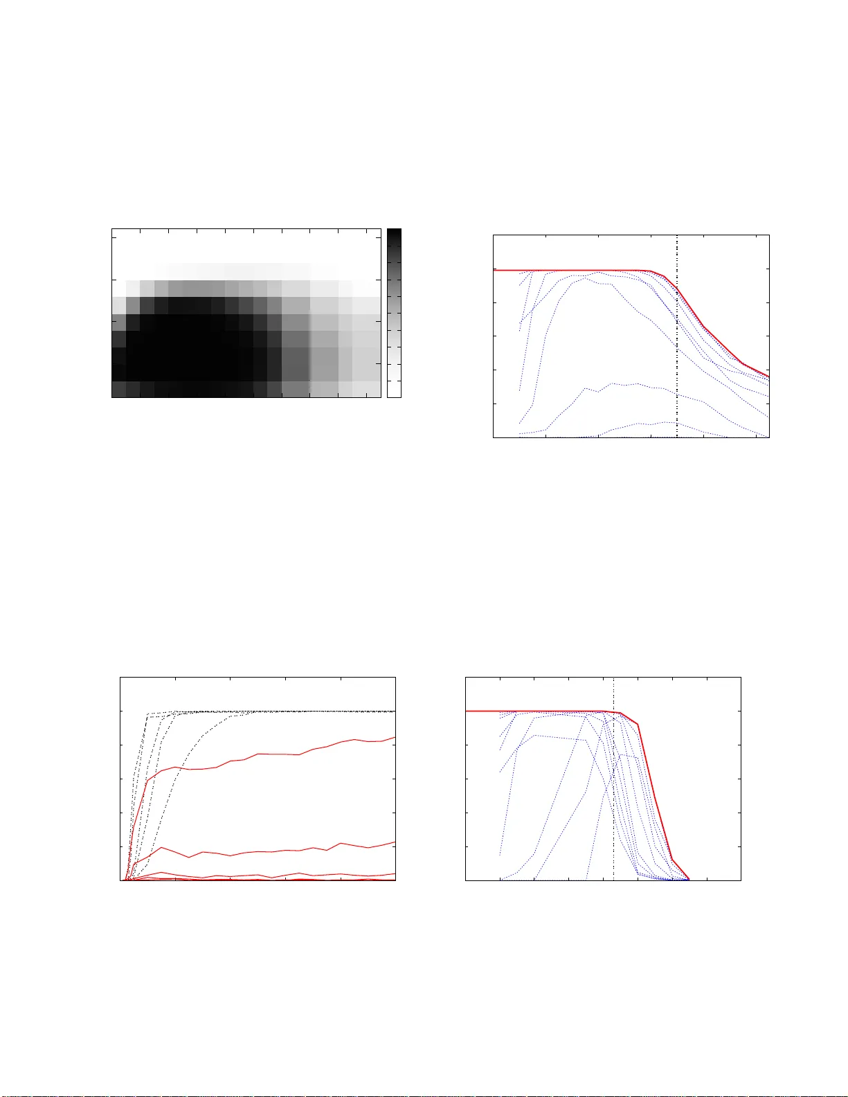
On the trade-oﬀ b et w een complexit y and correlation deca y in structural learning algor i thms Jos ´ e Ben to ∗ and Andrea Mon tanari † No v ember 15, 2021 Abstract W e consider the pro blem of learning the s tructure of Ising mo dels (pairwise binary Markov random ﬁelds) from i.i.d. samples . While several metho ds hav e been pro p o sed to acco mplish this task, their relative merits and limitations remain somewhat obs cure. By a nalyzing a num b er of concrete examples, we show that lo w-co mplexity algor ithms often fa il when the Mark ov r andom ﬁeld dev elo ps long-range correlations. Mo re precisely , this phenomenon appears to be re lated to the Ising mo del phase tr ansition (although it does not coincide with it). 1 In tro du ction and main results Giv en a graph G = ( V = [ p ] , E ), and a p ositiv e parameter θ > 0 the ferr omagnetic Ising mo del on G is the pairwise Mark ov random ﬁ eld µ G,θ ( x ) = 1 Z G,θ Y ( i,j ) ∈ E e θ x i x j (1) o v er binary v ariables x = ( x 1 , x 2 , . . . , x p ), x i ∈ { +1 , − 1 } . Apart from b eing one of the b est studied mo dels in statistical mec hanics [1, 2], the Ising mod el is a protot ypical undirected graphical mo d el. Since the seminal work of Hopﬁeld [3] and Hin ton and Sejnowski [4], it has found app lication in n u m erous areas of m ac hine learning, computer vision, clustering and sp atial statistics. The ob vious generali zation of the distribution (1) t o edge-dep end en t parameters θ ij , ( i, j ) ∈ E is of cen tral in terest in such applications, and will b e in tro duced in Section 2.2.2. Let us stress that we follo w the statistical mechanics con ven tion of calling (1) an Ising mo del ev en if the graph G is not a grid. In this p ap er we stud y the follo wing structural learning problem: Given n i.i.d. samples x (1) , x (2) ,. . . , x ( n ) ∈ { +1 , − 1 } p with distribution µ G,θ ( · ) , r e c on- struct the gr aph G . F or the sake of simplicit y , we assu me in most of the p ap er that the parameter θ is kno wn, and that G has no double edges (it is a ‘simple’ graph). W e fo cu s therefore on the k ey challe n ge of learning the graph stru cture asso ciated to the measure µ G,θ ( · ). This structur e is particularly imp ortant ∗ Department of Electrical Engineering, St an ford Universit y † Departments of Electrical Engineering and S tatistics, Stanford Un ivers ity 1 for extracting the qualitativ e features of the mo del, since it enco des its conditional indep end en ce prop erties. It follo ws from the general theory of exp onenti al families that, for any θ ∈ (0 , ∞ ), the mo del (1 ) is iden tiﬁable [5]. In particular, the str uctural learning problem is solv able with unboun ded sample complexit y and computational resources. The question we address is: for whic h classes of graphs and v alues of the parameter θ is the problem solv able under realistic complexit y constraints? More precisely , giv en an algorithm Al g , a graph G , a v alue θ of the mo del parameter, and a small δ > 0, the sample complexity is d eﬁned as n Alg ( G, θ ) ≡ inf n n ∈ N : P n,G,θ { Alg ( x (1) , . . . , x ( n ) ) = G } ≥ 1 − δ o , (2) where P n,G,θ denotes pr obabilit y with resp ect to n i.i.d. samp les with distribution µ G,θ . F urther , w e let χ Alg ( G, θ ) denote the n u m b er of op erations of the algorithm Alg , when ru n on n Alg ( G, θ ) samples. The general problem is ther efore to c haracterize the fun ctions n Alg ( G, θ ) and χ Alg ( G, θ ), and to design algorithms that m inimize the complexit y . Let us emph asize that these are n ot the only p ossible d eﬁnitions of sample and compu ta- tional complexit y . Alternativ e deﬁnitions are obtained by r equiring that the reconstructed str u cture Alg ( x (1) , . . . , x ( n ) ) is only partially corr ect. Ho w ever, for the algorithms consid ered in this p ap er, suc h deﬁnitions should not result in qualitativ ely d iﬀeren t b eha vior 1 General up p er and low er b ounds on the sample complexit y n Alg ( G, θ ) w ere prov ed by S an thanam and W ain wright [6, 7], without ho wev er taking in to accoun t computational complexit y . On the other end of the sp ectrum, sev eral lo w complexit y algorithms hav e b een develo p ed in the last few yea rs (see Section 1.3 for a b rief ov erview). Ho wev er the resulting sample complexit y b ound s on ly hold under sp eciﬁc assump tions on the und erlying mo del (i.e. on the pair ( G, θ )). A general un derstanding of the trade-oﬀs b et we en sample complexit y and computational complexit y is largely lacki n g. This p ap er is dev oted to the study of the tradeoﬀ b etw een sample complexit y and computational complexit y for some sp eciﬁc str u ctural learnin g algorithms, when applied to the Ising mo del. An imp ortant chall enge consists in the fact that the m o del (1) induces subtle correlations b et ween the binary v ariables ( x 1 , . . . , x p ). Th e ob jectiv e of a s tructural learning algorithm is to disenta n gle pairs x i , x j that are conditionally ind ep endent giv en the other v ariables (and hence are not connected b y an edge) from those that are instead conditionally d ep endent (and hence connected by an edge in G ). This b ecomes particularly diﬃcult w hen θ b ecomes large and h ence pairs x i , x j that are not connected by an edge in G b ecome strongly d ep endent. The n ext section sets the stage f or our wo r k b y discussing a simp le and concrete illustration of this phenomenon. 1.1 A to y example As a to y illustration 2 of the c hallenges of stru ctural learning, we will study the tw o families of graphs in Figure 1. The t w o families will b e d enoted by { G p } p ≥ 3 and { G ′ p } p ≥ 3 and are indexed b y the n u mb er of vertic es p . Graph G p has p v ertices and 2( p − 2) edges. Two of the v ertices (verte x 1 and v ertex 2) ha v e degree ( p − 2), and ( p − 2) ha ve degree 2. Graph G ′ p has also p vertic es, but only one edge b et we en vertic es 1 and 2. In other w ord s, grap h G ′ p corresp onds to v ariables x 1 and x 2 in teracting ‘directly’ (and hence n ot conditionally ind ep endent), while graph G p describ es a situation in whic h the tw o v ariables 1 Indeed t he algorithms considered in this p ap er reconstruct G by separately estimating the neighborho o d of eac h nod e i . This implies that any signiﬁcant p robabilit y of error results in a substantially d iﬀerent graph. 2 A similar example w as considered in [8]. 2 Figure 1: Two families of graph s G p and G ′ p whose distributions µ G p ,θ and µ G ′ p ,θ ′ merge as p gets large. in teract ‘indir ectly’ through numerous w eak int erm ediaries (b ut still are cond itionally indep endent since they are not connected). Fix p , and assu m e that one of G p or G ′ p is c hosen rand omly and i.i.d. samples x (1) ,. . . , x ( n ) from the corresp onding Ising distribution are giv en to u s. Can we eﬃciently d istinguish the t wo graphs, i.e. infer w h ther the s amples were generated us in g G p or G ′ p ? As men tioned ab ov e, since the mo del is iden tiﬁable, this task can b e ac hieve d with unboun ded sample and compu tational complexit y . F urther, since mo del (1) is an exp onentia l family , the p × p matrix of empirical co v ariances (1 /n ) P n ℓ =1 x ( ℓ ) ( x ( ℓ ) ) T pro vides a suﬃ cien t statistic for inferring the graph structure. In this sp eciﬁc example, w e assu me that diﬀeren t edge strengths are used in the tw o graphs: θ for graph G p and θ ′ for grap h G ′ p (i.e. we h av e to d istinguish b etw een µ G p ,θ and µ G ′ p ,θ ′ ). W e claim that, b y p rop erly c h o osing the p arameters θ and θ ′ , w e can ensure that the co v ariances appro ximately matc h | E G p ,θ { x i x j } − E G ′ p ,θ ′ { x i x j }| = O (1 / √ p ). Indeed the same r emains true for all marginals in vol vin g a b ounded num b er of v ariables. Namely , for all subsets of ve r tices U ⊆ [ p ] of b ound ed size | µ G p ,θ ( x U ) − µ G ′ p ,θ ′ ( x U ) | = O (1 / √ p ). Lo w-complexit y algorithms typically estimate eac h edge usin g only a small sub set lo w–dimensional m arginal. Hence, they are b ound to fail un less the num b er of samples n d iv erges with the graph size p . On the other hand, a n aiv e information-theoretic lo wer b ound (in the spir it of [6 , 7]) on ly yields n Alg ( G, θ ) = Ω(1). This sample complexit y is ac hiev able b y using global statistic s to d istinguish the tw o graph s. In other words, ev en for this simple examp le, a dic hotom y emerges: either a n umb er of samp les has to gro w with the num b er of parameters, or algorithms h a v e to exploit a large num b er of m arginals of µ G,θ . T o conﬁrm our claim, we need to compute the co v ariance of the Ising measures d istributions µ G p ,θ , µ G ′ p ,θ ′ . W e easily obtain, for the latter graph E G ′ p ,θ ′ { x 1 x 2 } = tanh θ ′ , (3) E G ′ p ,θ ′ { x i x j } = 0 . ( i, j ) 6 = (1 , 2) . (4) The calcula tion is somewh at more in tricate for graph G p , so w e d efer complete formulae to App end ix A and rep ort here only the result for p ≫ 1, θ ≪ 1: E G p ,θ { x 1 x 2 } = tanh  pθ 2 + O ( pθ 4 , θ )  , (5) E G p ,θ { x i x j } = O ( θ , pθ 3 ) , i ∈ { 1 , 2 } , j ∈ { 3 , . . . , p } , (6) E G p ,θ { x i x j } = O ( θ 2 , pθ 4 ) , i, j ∈ { 3 , . . . , p } . (7) In other words, v ariables x 1 and x 2 are strongly correlated (although not connected), while all th e 3 other v ariables are wea kly correlated. By letting θ = p θ ′ /p this co v ariance structure matc hes Eqs. (3), (4 ) up to correctio n s of order 1 / √ p . Notice that the am biguit y b et ween the t wo mo d els G p and G ′ p arises b ecause seve r al weak, indir ect paths b et ween x 1 and x 2 in graph G p , add u p to the same eﬀect as a strong direct connection. Th is to y example is hence suggestiv e of the general phenomenon that strong long-range correlations can ‘fak e’ a direct connection. Ho wev er, the example is not completely convincing for sev eral reasons: 1. Most algorithms of in terest estimate eac h edge on the b asis of a large num b er of lo w -d imensional marginals (for instance al l pairwise correlations). 2. Reconstruction guarantee s ha ve b een p ro ve d for graphs with b ounded degree [9, 10, 6, 7, 11], while here we are letting th e m axim um degree b e as large as the system size. Notice ho wev er that a th e graph considered here are only sparse ‘on av erage’. 3. It ma y app ear that the diﬃculty in distingu ish ing grap h G p from G ′ p is r elated to the fact that in the former w e tak e θ = O (1 / √ p ). This is ho wev er the natural scaling when the degree of a vertex is large, in order to obtain a non-trivial distribution. If the grap h G p had θ b ound ed a wa y from 0, this wo u ld resu lt in a distr ibution µ G p ,θ ( x ) concent r ated on the t wo anti p o dal conﬁgurations: all-(+1) and all-( − 1). Stru ctur al learning would b e equ ally diﬃcult in this case. Despite these p oints, this mo d el pro vid es already a useful counte r -example. I n App endix D.3 we will sho w wh y , even for b oun ded p (and hence θ b oun ded aw a y from 0) the mo d el G p in Figure 1 ‘f o ols’ regularized logistic regression algorithm of Ra vikum ar, W ain wright and Laﬀerty [11]. Regularized logistic regression r econstructs G ′ p instead of G p . 1.2 Outline of the pap er The rest of this pap er is dev oted to b oun d ing the sample complexit y n Alg and computational com- plexit y χ Alg for a num b er of graph mo d els, as a function of θ . Results of this an alysis are pr esented in Section 2 for thr ee algorithms: a sim p le thresholding algorithm, th e conditional ind ep endence test metho d of [10 ] and th e p en alized pseud o-lik eliho o d metho d of [11]. In Section 3, w e v alidate our analysis through numerical sim ulations. Finally , S ection 4 con tains the p ro ofs with some tec h n ical details deferred to the app endices. This analysis unv eils a general pattern: when the mo del (1) develops str ong c orr elations, sever al low-c omplexity algor ithms fail, or r e qu ir e a lar ge numb er of samples. What do es ‘strong correlations’ mean? As the to y example in the previous s ection demonstr ates, correlations arise from a trade-oﬀ b et ween the degree (whic h we will c haracterize here via the maximum degree ∆), and the in teraction strength θ . It can b e ascrib ed to a few strong connections (large θ ) or to a large n umb er of weak connections (large ∆). Is there any meaningful w a y to compare and com bin e these quantit ies ( θ and ∆)? An answ er is suggested by the theory of Gibbs measures wh ic h p redicts a dr amatic change of b ehavi or wh en θ crosses the so-called ‘uniqu eness th r eshold’ θ uniq (∆) = atanh (1 / (∆ − 1)) [12]. F or θ < θ uniq (∆) Gibb s sampling mixes rapidly and f ar apart v ariables in G are r oughly indep endent [13]. Vice ve r s a, for any θ > θ uniq (∆) th ere exist graph families on wh ic h Gibbs sampling is slo w , and far apart v ariables are strongly d ep endent [14]. While p olynomial samp ling algorithms exists for all θ > 0 [15 ], for θ < 0, in the r egime | θ | > θ uniq (∆) sampling is arguably #-P h ard [16]. Related to the un iqueness thresh old is also the phase transition threshold, wh ic h is graph dep endent, with t ypically θ crit ≤ const ./ ∆. W e will see that th is is indeed a r elev ant w a y of comparing interac tion stren gth and degree, ev en f or s tr uctural learning. A l the algorithms we analyzed (men tioned ab o ve ) prov ably fail for 4 θ ≫ const ./ ∆, for a num b er of ‘natural’ graph families. Our work raises sev eral fascinating questions, the most imp ortan t b eing the constru ction of structur al learning algorithm with pro v able p erformance guaran tees in the strongly d ep endent regime θ crit ≫ const ./ ∆. The question as to whether such an algorithm exists is left op en by th e presen t pap er (but see next section for an o verview of earlier w ork). Let u s ﬁnally emp hasize that w e do not think that any of the sp eciﬁc families of graphs studied in the present pap er is intrinsical ly ‘hard’ to learn. F or ins tance, w e sho w b elo w that the regularized logistic regression metho d of [11] fails on r andom regular graphs, while it is easy to learn su c h graph s using the simple thresholding algorithm of Section 2.1. The sp eciﬁc families w h ere indeed c hosen mostly b ecause they are analytica lly tractable. 1.3 F urther related w ork T r aditional algorithms for learnin g Ising mo dels we r e d ev elop ed in the con text of Boltzmann mac hines [4, 17, 18]. These algorithms tr y to solv e the maxim u m lik eliho o d p roblem b y gradien t ascent. Estimating the gradient of the log-lik elihoo d fun ction requires to compute exp ectatio n s with resp ect to the Is ing distrib ution. In these w orks, th is w as d one usin g the Marko v Chain Monte Carlo (MCMC) metho d , and more sp eciﬁcally Gibbs sampling. W e shall not consider this approac h in ou r stud y for t w o type of r easons. First of all, it do es not output a ‘structure’ (i.e. a spars e sub set of the  p 2  p oten tial ed ges): because of approximat ion errors, it yields non -zero v alues for all the edges. Th is problem can in p rinciple b e o vercome by u sing suitably regularized ob jectiv e functions, but s u c h a mo diﬁed algorithm was nev er studied. Second, the need to compute exp ectation v alues with resp ect to the Ising d istribution, an d the use of MCMC to ac hieve this goal, p oses some fund amen tal limitations. As men tioned ab ov e, the Mark o v c hain commonly used b y th ese metho ds is simp le Gibb s sampling. T his is known to hav e mixing time that gro ws exp onen tially in th e n umb er of v ariables for θ > θ uniq (∆), and h en ce d o es n ot yield go o d estimates of the exp ectation v alues in practice. While p olynomial samp ling schemes exist for mo dels with θ > 0 [15], they do not apply to θ < 0 or to general mo dels with edge-dep en den t parameters θ ij . Already in the case θ < 0, estimating exp ectation v alues of the I sing distr ibution is lik ely to b e #-P hard [16 ]. Abb eel, Koller and Ng [9] ﬁrst dev elop ed a metho d with computational complexit y prov ably p oly- nomial in th e n u m b er of v ariables, for b ou n ded maxim um d egree, and logarithmic sample complexit y . Their approac h is based on ingenious u se of the Hammersley-Cliﬀord r epresen tation of Marko v Ran- dom Fields. Un f ortunately , the computational complexit y of this approac h is of ord er p ∆+2 whic h b ecomes unpractical for reasonable v alues of the degree and net wo rk size (and sup erp olynomial for ∆ divergi n g with p ). The algorithm b y Bresler, Mossel and Sly [10] studied in S ection 2.2.1 pr esen ts similar limitations, that the authors o v ercome (in the small θ regime) by exploiting the corr elation deca y phenomenon. An alternativ e p oint of view consists in using standard regression metho ds. In the con text of Ising mo dels, Ra vikumar, W ain wright and Laﬀert y [11] sh ow ed that the neigh b orh o o d of a vertex i can b e eﬃcien tly reconstru cted b y solving an appropriate regularized regression problem. More precisely , the v alues of v ariable x i are regressed against the v alue of all the other v ariables. The logistic regression log-lik eliho o d is regularized by adding an ℓ 1 -p enalt y that promotes the selection of sparse graph structures. W e will analyze this metho d in Section 2.2.2. The ap p roac h of [11] extends to non-Gaussian mo dels earlier w ork by Meinshausen and B ¨ uhlmann [19]. Let us notice in passing that th e case of Gaussian graphical m o dels is substantia lly easier since the log-lik eliho o d of a give n mo del can b e ev aluated easily in this case [20]. A short ve r sion of this pap er was presented at th e 2009 Neural Information Pr o cessing Systems 5 symp osium . S ince then, at least t wo group s exp lored the c hallenges p ut forward in our w ork. Anan d - kumar, T an an d Willsky [21] p ro ve that, for sequ ences of random graph s whic h are sparse on a verage (i.e. w ith b oun ded av erage degree), structural learning is p ossible th roughout th e correlation deca y regime θ < θ crit . Th is result generalizes our analysis of random regular grap h s (see n ext section), to the more c h allenging case of graph s with random degrees. Co cco and Monasson [22] p rop osed and ‘adaptiv e cluster’ heur istics and demonstr ated emp irically go o d p erformances f or sp eciﬁc graph families, also for θ > θ crit . A mathematical analysis of their app roac h is lac kin g. 2 Results 2.1 The simple thresholding algorit hm In order to illustrate the inte r p la y b et wee n graph structure, sample complexit y and in teraction strength θ , it is instructive to consider a simple example. The thr esholding algorithm r econstructs G by thresh olding the emp irical correlations b C ij ≡ 1 n n X ℓ =1 x ( ℓ ) i x ( ℓ ) j , (8) for i, j ∈ V . Threshold ing ( samples { x ( ℓ ) } , threshold τ ) 1: Compute the empirical correlations { b C ij } ( i,j ) ∈ V × V ; 2: F or eac h ( i, j ) ∈ V × V 3: If b C ij ≥ τ , set ( i, j ) ∈ E ; W e w ill denote this algorithm by Thr ( τ ). Notice that its complexit y is dominated by the com- putation of the empirical correlations, i.e. χ Thr ( τ ) = O ( p 2 n ). The sample complexit y n Thr ( τ ) can b e b ound ed for sp eciﬁc classes of graph s as follo ws (for pro ofs see Section 4.2 ). Theorem 2.1. If G is a tr e e, and τ ( θ ) = (tanh θ + tanh 2 θ ) / 2 , then n Thr ( τ ) ( G, θ ) ≤ 32 (tanh θ − tanh 2 θ ) 2 log 2 p δ . (9) Theorem 2.2. If G has maximum de gr e e ∆ > 1 and if θ < atanh(1 / (2∆)) then ther e exists τ = τ ( θ ) such that n Thr ( τ ) ( G, θ ) ≤ 32 (tanh θ − 1 2∆ ) 2 log 2 p δ . (10) F urther, the choic e τ ( θ ) = (tanh θ + (1 / 2∆)) / 2 achieves this b ound. Theorem 2.3. Ther e exists a numeric al c onstant K such that the fol lowing is true. If ∆ > 3 and θ > K/ ∆ , ther e ar e gr aphs of b ounde d de gr e e ∆ such that for any τ , n Thr ( τ ) = ∞ , i.e. the thr esholding algorithm always fails with high pr ob ability. These results conﬁ rm the idea that the f ailure of low-c omplexity algorithms is r elated to long- range correlations in th e und erlying graphical mo d el. If th e graph G is a tree, then correlations b et ween far apart v ariables x i , x j deca y exp onen tially with the distance b et ween vertice s i , j . Hence trees can b e learn t from O (log p ) samples irresp ectiv ely of their top ology and maxim u m degree (assuming θ 6 = ∞ ). The same happ ens on b ounded -d egree graphs if θ ≤ const ./ ∆. Ho w ev er, for θ > const ./ ∆, ther e exists families of b ounded degree graphs with long-range correlations. 6 2.2 More sophisticated algorithms In this section w e c haracterize χ Alg ( G, θ ) and n Alg ( G, θ ) for more adv anced algorithms. W e again obtain v ery distinct b ehavi ors of these algorithms dep ending on the strength of correlations. W e fo cus on t wo t yp e of algorithms and only include the pro of of our most c hallenging result, Theorem 2.8 (for th e pro of see Section 4.3). In the follo win g we d enote b y ∂ i the n eigh b orho o d of a no d e i ∈ G ( i / ∈ ∂ i ), and assume the degree to b e b ounded: | ∂ i | ≤ ∆. 2.2.1 Lo cal Indep endence T est A recur r ing approac h to stru ctural learning consists in exploiting the conditional in dep end ence struc- ture enco ded b y the graph [9, 10, 23, 24]. Let us consider, to b e d eﬁnite, the appr oac h of [10], sp ecializing it to th e mo del (1). Fix a vertex r , wh ose neigh b orho o d we w ant to reconstruct, and consider the conditional d istribution of x r giv en its neighbors 3 : µ G,θ ( x r | x ∂ r ). An y change of x i , i ∈ ∂ r , pro d uces a c hange in this d istribution wh ic h is b ounded a w a y from 0. Let U b e a candidate neigh b orho o d , and assume U ⊆ ∂ r . Then c h anging the v alue of x j , j ∈ U will p ro duce a n oticeable change in the marginal of X r , ev en if w e condition on the remaining v alues in U and in an y W , | W | ≤ ∆ . On the other hand, if U * ∂ r , then it is p ossible to ﬁ n d W (with | W | ≤ ∆) and a no de i ∈ U su c h that, c hanging its v alue after ﬁxing all other v alues in U ∪ W will pr o duce no n oticeable c hange in the conditional marginal. (Just choose i ∈ U \ ∂ r and W = ∂ r \ U ). This pro cedure allo w s us to distinguish subsets of ∂ r f rom other sets of v ertices, th us m otiv ating th e follo wing algorithm. Local Ind ependen ce Test ( samples { x ( ℓ ) } , th r esholds ( ǫ, γ ) ) 1: Select a no de r ∈ V ; 2: Set as its neigh b orh o o d the largest candid ate neighbor U of size at most ∆ for which the s core function S core ( U ) > ǫ/ 2; 3: Rep eat for all no des r ∈ V ; The score f unction Score ( · ) dep ends on ( { x ( ℓ ) } , ∆ , γ ) and is d eﬁ ned as follo ws, min W,j max x i ,x W ,x U ,x j | b P n,G,θ { X i = x i | X W = x W , X U = x U }− b P n,G,θ { X i = x i | X W = x W , X U \ j = x U \ j , X j = x j }| . (11) In the min im um, | W | ≤ ∆ and j ∈ U . In the maxim um, the v alues m ust b e su c h that b P n,G,θ { X W = x W , X U = x U } > γ / 2 b P n,G,θ { X W = x W , X U \ j = x U \ j , X j = x j } > γ / 2 (12) b P n,G,θ is the emp irical distribu tion calculated fr om the samp les { x ( ℓ ) } n ℓ =1 . W e denote this algorithm b y Ind ( ǫ, γ ). The searc h ov er candidate n eighb ors U , the searc h for minima and maxima in the computation of the S core ( U ) and the compu tation of b P n,G,θ all con tribu te for χ Ind ( G, θ ). Both theorems that follo w are consequences of the analysis of [10], hence omitted. 3 If a is a vector and R is a set of indices then we denote b y a R the vector formed by the components of a with ind ex in R . 7 Theorem 2.4. L et G b e a gr aph of b ounde d de gr e e ∆ ≥ 1 . F or every θ ther e exists ( ǫ, γ ) , and a numeric al c onsta nt K , such that n Ind ( ǫ,γ ) ( G, θ ) ≤ 100∆ ǫ 2 γ 4 log 2 p δ , (13) χ Ind ( ǫ,γ ) ( G, θ ) ≤ K (2 p ) 2∆+1 log p . (14) Mor e sp e ciﬁc al ly, one c an take ǫ = 1 4 sinh(2 θ ) , γ = e − 4∆ θ 2 − 2∆ . This ﬁrs t r esult implies in particular that G can b e reconstructed with p olynomial complexit y for an y b ounded ∆. Ho wev er, the degree of such p olynomial is p rett y high and non-uniform in ∆. This makes the ab ov e app roac h impractical. A wa y out was p rop osed in [10]. The id ea is to iden tify a set of ‘p otentia l neigh b ors’ of v ertex r via thresholdin g: B ( r ) = { i ∈ V : b C r i > κ/ 2 } . (15) F or eac h no d e r ∈ V , we ev aluate Score ( U ) by restricting the minimum in Eq. (11) o ver W ⊆ B ( r ), and searc h only ov er U ⊆ B ( r ). W e call this algorithm IndD ( ǫ, γ , κ ). Th e basic int u ition here is th at C r i decreases rapidly with the graph d istance b etw een ve r tices r and i . As menti oned ab o v e, this is true at low temp erature. Theorem 2.5. L et G b e a gr aph of b ounde d de gr e e ∆ ≥ 1 . Assume that θ < K / ∆ for some smal l enough c onsta nt K . Then ther e exists ǫ, γ , κ such that n IndD ( ǫ,γ ,κ ) ( G, θ ) ≤ 8( κ 2 + 8 ∆ ) log 4 p δ , (16) χ IndD ( ǫ,γ ,κ ) ( G, θ ) ≤ K ′ p ∆ ∆ log(4 /κ ) α + K ′ ∆ p 2 log p . (17) Mor e sp e ciﬁc al ly, we c an take κ = tanh θ , ǫ = 1 4 sinh(2 θ ) and γ = e − 4∆ θ 2 − 2∆ . 2.2.2 Regularized Pseudo-Lik eliho o ds A diﬀerent app roac h to the learning p roblem consists in maximizing an app ropriate empirical like li- ho o d f unction [11, 25, 26, 27, 19, 28]. In order to con trol statistical ﬂuctuations, and select sparse graphs, a regularizat ion term is often added to th e cost fu nction. As a sp eciﬁc lo w complexit y implemen tation of this idea, we consider the ℓ 1 -regularized pseud o- lik eliho o d metho d of [11 ]. F or eac h n o de r , th e follo wing likeli h o o d function is considered L ( θ ; { x ( ℓ ) } ) = − 1 n n X ℓ =1 log P n,G,θ ( x ( ℓ ) r | x ( ℓ ) \ r ) (18) where x \ r = x V \ r = { x i : i ∈ V \ r } is the v ector of all v ariables except x r and P G,θ is deﬁ ned from the follo win g extension of (1), µ G,θ ( x ) = 1 Z G,θ Y i,j ∈ V e θ ij x i x j (19) where θ = { θ ij } i,j ∈ V is a ve ctor of r eal parameters. Mo d el (1) corresp ond s to θ ij = 0 , ∀ ( i, j ) / ∈ E and θ ij = θ , ∀ ( i, j ) ∈ E . The fun ction L ( θ ; { x ( ℓ ) } ) dep en ds only on θ r, · = { θ r j , j ∈ ∂ r } and is used to estimate the neigh b orho o d of eac h no de by the follo wing algorithm, Rlr ( λ ), 8 Regularized Logistic Regre ssion ( samples { x ( ℓ ) } , regularization ( λ )) 1: Select a no de r ∈ V ; 2: Calculate ˆ θ r, · = arg min θ r, · ∈ R p − 1 { L ( θ r, · ; { x ( ℓ ) } ) + λ k θ r, · k 1 } ; 3: If ˆ θ r j > 0, set ( r, j ) ∈ E ; Our ﬁrst result sho ws that Rlr ( λ ) indeed reconstructs G if θ is suﬃ cien tly sm all. Theorem 2.6. Ther e exists numeric al c onstants K 1 , K 2 , K 3 , such that the fol lowing i s true. L et G b e a gr aph with de gr e e b ounde d by ∆ ≥ 3 . If θ ≤ K 1 / ∆ , then ther e exist λ such that n Rlr ( λ ) ( G, θ ) ≤ K 2 θ − 2 ∆ log 8 p 2 δ . (20) F urther, the ab ove holds with λ = K 3 θ ∆ − 1 / 2 . This th eorem is pr o v ed b y noting that for θ ≤ K 1 / ∆ correlations deca y exp onenti ally , whic h mak es all conditions in Theorem 1 of [11] (denoted there by A1 and A2) hold, and then computing the probab ility of success as a function of n with sligh tly more care. The details of the pro of are written in App endix B. In order to pro ve a con v erse to the ab o ve result, we n eed to make some assump tions on λ . Deﬁnition 2.7. Given θ > 0 , we say th at λ i s reasonable for that value of θ if the fol lowing c ondition s hold: ( i ) Rlr ( λ ) is suc c essful with pr ob ability lar ger than 1 / 2 on any star gr aphs (a g r aph c omp ose d by a vertex r c onne cte d to ∆ neighb ors, plus isolate d vertic es) if n is chosen suﬃciently high; ( ii ) λ ≤ δ ( n ) for some se quenc e δ ( n ) ↓ 0 . In other words, assumption ( i ) requires the algorithm to b e successful on a particularly simple class of graphs, and hence do es not en tail an y loss of generalit y . Assumption ( ii ) enco des ins tead the standard wa y of scaling regularization terms, by letting them v anish as the n umb er of samples increases. Th is is necessary in order to get asymptotic consistency of the parameter v alues θ ij . With these assu mptions w e can s tate th e follo w in g con verse theorem, whose pro of is deferred to Section 4.3. Theorem 2.8. Ther e e xi sts a numeric al c onstant K such that the fol lowing happ ens. If θ > K/ ∆ , ∆ > 3 , then ther e exists g r aphs G of de gr e e b ounde d by ∆ such tha t for al l r e asonable λ , n Rlr ( λ ) ( G ) = ∞ , i.e. r e gularize d lo gistic r e gr ession fails with high pr ob ability. The grap h s f or wh ic h regularized logistic regression fails are not con triv ed examples. In deed, as part of the pro of of Theorem 2.8, and as prov ed in App en d ix D, w e hav e the follo wing facts ab out Rlr ( λ ): • If G is a tree, th en Rl r ( λ ) reco ver G w ith high pr obabilit y for any θ (for a suitable λ ); • F or eve r y graph G p in the family describ ed in Section 1.1, R lr ( λ ) fails with high pr obabilit y for θ large enough and for all λ ; • If G is s amp led u niformly from the ensemble of regular graphs Rlr ( λ ) fails with high probabilit y for θ large enou gh and λ ‘r easonable’; • if G is a large t wo dim en sional grid It fails with h igh probabilit y for θ large enough and λ ‘reasonable’. 9 W e note here that T h eorem 2.8 relies on pro ving th at a so-calle d ‘Incoherence condition’ is necessary for Rlr to successfully reconstru ct G . Although a similar result w as prov en in [29] for mo del selection usin g the Lasso, this p ap er is the ﬁrst to prov e that a similar Incoherence condition is also n ecessary when the u nderlying mo del is the Ising mo del. The intuition b ehin d this is quite simple. Begin b y noticing that w hen n → ∞ , and under th e restriction that λ → 0, solutions giv en by Rl r con ve rge to θ ∗ as n → ∞ [11]. Hence, for large n , w e can expand L in a quadratic function cen tered aroun d θ ∗ plus a small sto chasti c error term. Consequent ly , when adding the regularizatio n term to L , we obtain cost function analogous to the Lasso plus an error term that needs to b e control led. Th e study of the dominating con tribu tion leads to the incoherence condition. In general there are no p ractical w ays to ev aluate the incoherence condition for a giv en graph ical mo del. This requires in fact to compute exp ectations with r esp ect to the Ising distr ib ution. As discussed ab ov e, this is hard for | θ | > θ uniq (∆). Hence this condition was not chec k ed for families of graphs. A large part of our tec h nical con tribution consists indeed in ﬁlling this gap. T o this end, we use to ols from mathematical statistica l mec hanics, namely lo w temp erature series for Ising mo dels on grids [30, 31], and lo cal w eak conv ergence r esults for Ising mo dels on r an d om graphs [32, 33]. 3 Numerical exp erimen ts In order to explore the practical relev ance of the ab o ve results, w e carried out extensiv e numerical sim ulations usin g the regularized logistic regression algorithm Rlr ( λ ). Among other learning algo- rithms, Rlr ( λ ) s tr ik es a go o d balance of complexit y and p erformance. S amples f rom th e Ising mo d el (1) where generated usin g Gibbs sampling (a.k.a. Glaub er dynamics). Mixing time can b e ve r y large for θ ≥ θ uniq , and wa s estimated using the time requir ed for th e o verall b ias to c hange sign (this is a quite conserv ativ e estimate at lo w temp erature). Generating the samples { x ( ℓ ) } w as indeed the b ulk of our computational eﬀort and to ok ab out 50 da ys CPU time on Pe ntium Dual Core pr o cessors. Notice that Rlr ( λ ) had b een tested in [11] only on tree graph s G , or in the w eakly coup led regime θ < θ uniq . In th ese cases sampling from the Is ing mo del is easy , but structural learning is also in trins ically easier. Figure rep orts the su ccess probabilit y of Rlr ( λ ) when applied to r andom subgraphs of a 7 × 7 t wo -dimen sional grid. Each su c h graphs w as obtained b y remo ving eac h edge indep endent ly with probabilit y ρ = 0 . 3. Success probability wa s estimated b y applying Rlr ( λ ) to eac h vertex of 8 graph s (th us av eraging o ve r 392 runs of Rlr ( λ )), u sing n = 4500 samples. W e scaled the regularization parameter as λ = 2 λ 0 θ (log p/n ) 1 / 2 (this choice is m otiv ated by the algorithm analysis [11] and is empirically the most satisfactory), and searc hed ov er λ 0 . The d ata clearly illustrate the phenomenon discussed in the previous pages. Despite th e large n u mb er of samples n ≫ log p , wh en θ crosses a threshold, the algorithm starts p erformin g p o orly irresp ectiv e of λ . In tr iguin gly , this th reshold is not f ar from the critical p oin t of the Ising mo d el on a rand omly diluted grid θ crit ( ρ = 0 . 3) ≈ 0 . 7 [34, 35]. Figure 3 p resen ts similar d ata wh en G is a uniformly random graph of d egree ∆ = 4, o ver p = 50 v ertices. The ev olution of the su ccess probabilit y with n clearly sho w s a dic hotomy . When θ is b elo w a threshold, a small num b er of samples is suﬃcient to reconstruct G with h igh probabilit y . Ab o ve the threshold ev en n = 10 4 samples are to few. In this case we can p redict the thresh old analytically , cf. Lemma 4.3 b elo w, and get θ thr (∆ = 4) ≈ 0 . 4203 , w hic h compares fa vo r ably with the data. 10 0 0.1 0.2 0.3 0.4 0.5 0.6 0.7 0.8 0.9 1 0.1 0.2 0.3 0.4 0.5 0.6 0.7 0.8 0.9 1 5 10 15 20 0 0.2 0.4 0.6 0.8 1 1.2 0 0.2 0.4 0.6 0.8 1 λ 0 θ θ P succ Figure 2: Learning random subgraph s of a 7 × 7 ( p = 49) t wo-dimensional grid from n = 4500 Ising mo d els samples, using regularized logistic regression. Left: su ccess pr obabilit y as a fun ction of the mo del p arameter θ and of the regularization parameter λ 0 (dark er corresp ond s to highest probabilit y). Righ t: the same data plotted for several choice s of λ v ersus θ . T h e vertica l line corresp onds to the mo d el critical temp erature. Th e thick line is an env elop e of the curv es obtained for diﬀerent λ , and should corresp ond to optimal regularizati on. 0 0.2 0.4 0.6 0.8 1 1.2 0 2000 4000 6000 8000 10000 0 0.2 0.4 0.6 0.8 1 1.2 0 0.1 0.2 0.3 0.4 0.5 0.6 0.7 0.8 P succ θ = 0 . 10 θ = 0 . 15 θ = 0 . 45 θ = 0 . 45 n θ P succ Figure 3: Learning uniformly random graphs of degree ∆ = 4 from Ising mo dels samples, usin g regularized logistic regression. Left: success pr obabilit y as a fu nction of th e num b er of samples n for sev eral v alues of θ . Dott ed: θ = 0 . 10, 0 . 15, 0 . 20, 0 . 35, 0 . 40 (in all these cases θ < θ thr (∆ = 4)). Dashed: θ = 0 . 45, 0 . 50, 0 . 55, 0 . 60, 0 . 65 ( θ > θ thr (4), some of these are ind istinguishable from the axis). Righ t: the s ame data p lotted for seve r al c hoices of λ versus θ as in Fig. 2 , righ t p anel. 11 4 Pro ofs 4.1 Notation and impor tan t remarks Before pro ceeding it is con venien t to in tro d uce some notation and m ak e s ome imp ortant remarks. If V is a matrix and R is an in dex set then V R denotes the v ector formed by all ent r ies wh ose index lies in R and similarly , if M is a matrix and R, P are ind ex sets then M R P denotes the su bmatrix with ro w indices in R and column indices in P . As b efore, we let r b e the ve r tex whose neigh b orho o d w e are trying to reconstru ct and deﬁne S = ∂ r and S c = V \ ∂ r ∪ r . S ince the cost fun ction L ( θ ; { x ( ℓ ) } ) + λ k θ k 1 only dep ends on θ throu gh its comp on ents θ r, · = { θ r j } , we will hereafter neglect all the other parameters and w rite θ as a shorth and of θ r, · . Let ˆ z ∗ b e a sub gradien t of k θ k 1 ev aluated at the tru e p arameters v alues, θ ∗ = { θ r j : θ ij = 0 , ∀ j / ∈ ∂ r , θ r j = θ , ∀ j ∈ ∂ r } . Let ˆ θ n b e th e parameter estimate return ed by Rlr ( λ ) when the n u mb er of samples is n . Note that, s in ce we assum ed θ ∗ ≥ 0, we h av e θ ∗ S > 0 and hen ce ˆ z ∗ S = 1 . Deﬁne Q n ( θ ; { x ( ℓ ) } ) to b e the Hessian of L ( θ ; { x ( ℓ ) } ) and Q ( θ ) = lim n →∞ Q n ( θ ; { x ( ℓ ) } ). By the law of large n u mb ers Q ( θ ) exists a.s. and is the Hessian of E G,θ log P G,θ ( X r | X \ r ) where E G,θ is the exp ectation with r esp ect to (19) and X is a random v ariable d istributed according to (19). I t is con venien t to recall her e the expressions for the Hessian and gradient of L for ﬁn ite n and in the limit when n → ∞ . F or all i, j ∈ V \{ r } w e ha v e, Q n ij ( θ ) = 1 n n X ℓ =1 x ( ℓ ) i x ( ℓ ) j cosh 2  P t ∈ V \{ r } θ r t x ( ℓ ) t  , (21 ) Q ij ( θ ) = E G,θ ∗ X i X j cosh 2 ( P t ∈ V \{ r } θ r t X t ) ! , (22) [ ∇ L n ( θ )] i = 1 n n X ℓ =1 x ( ℓ ) i  tanh  X t ∈ V \{ r } θ r t x ( ℓ ) t  − x ( ℓ ) r  , (23) [ ∇ L ( θ )] i = E G,θ ∗ n X i tanh  X t ∈ V \{ r } θ r t X t o − E G,θ ∗ { X i X r } . (24) Note that from the last expression it follo ws that ∇ L ( θ ∗ ) = 0. W e will denote the maximum and minim um eigen v alue of a symmetric matrix M b y σ max ( M ) and σ min ( M ) resp ectiv ely . Recall that k M k ∞ = max i P j | M ij | . W e will omit argumen ts whenever clear from the con text. An y quantit y ev aluated at the true parameter v alues will b e repr esen ted with a ∗ , e.g. Q ∗ = Q ( θ ∗ ). Quantit ies under a ∧ dep end on n . When clear from the conte xt and since all the examples that we work on h a v e θ ij ∈ { 0 , θ } , we will write E G,θ as E G,θ or even simp ly E . S imilarly , P G,θ will b e sometimes written as simp ly P G,θ or just P . A s ubscript n und er P G,θ , i.e. P n,G,θ , will b e in tro duced to denote th e pro du ct m easure formed b y n copies of mo d el (19). Th rough out this section P succ will denote the p robabilit y of su ccess of a giv en algorithm, that is, the probabilit y th at the algorithm is able to reco v er the u n derlying G exactly . Throughout this section G is a graph of maximum degree ∆. 4.2 Simple Thresholding In the follo wing w e let C ij ≡ E G,θ { X i X j } wh ere exp ectation is tak en with resp ect to the Ising mo d el (1). 12 Pr o of. (Theorem 2.1 ) If G is a tree then C ij = tanh θ for all ( ij ) ∈ E and C ij ≤ tanh 2 θ for all ( ij ) / ∈ E . T o see th is notice that only paths th at connect i to j con tribute to C ij and giv en that G is a tree there is only one such path and its length is exactly 1 if ( i, j ) ∈ E and at least 2 wh en ( i, j ) / ∈ E . The p robabilit y that Thr ( τ ) fails is 1 − P succ = P n,G,θ { b C ij < τ for some ( i, j ) ∈ E or b C ij ≥ τ f or some ( i, j ) / ∈ E } . (25) Let τ = (tanh θ + tanh 2 θ ) / 2. Applying Azuma-Hoeﬀding inequalit y to b C ij = 1 n P n ℓ =1 x ( ℓ ) i x ( ℓ ) j w e ha ve that if ( i, j ) ∈ E then, P n,G,θ ( b C ij < τ ) = P n,G,θ n X ℓ =1 ( x ( ℓ ) i x ( ℓ ) j − C ij ) < n ( τ − tanh θ ) ! ≤ e − 1 32 n (tanh θ − tanh 2 θ ) 2 (26) and if ( i, j ) / ∈ E th en similarly , P n,G,θ ( b C ij ≥ τ ) = P n,G,θ n X ℓ =1 ( x ( ℓ ) i x ( ℓ ) j − C ij ) ≥ n ( τ − tanh 2 θ ) ! ≤ e − 1 32 n (tanh θ − tanh 2 θ ) 2 . (27) Applying union b ound o v er the t wo p ossibilities, ( i, j ) ∈ E or ( i, j ) / ∈ E , and o v er the edges ( | E | < p 2 / 2), we can b ound P succ b y P succ ≥ 1 − p 2 e − 1 32 n (tanh θ − tanh 2 θ ) 2 . (28) Imp osing the righ t h and side to b e larger than δ pro ves our result. Pr o of. (Theorem 2.2) W e w ill p ro ve th at, for θ < arctanh(1 / (2∆)), C ij ≥ tanh θ for all ( i, j ) ∈ E and C ij ≤ 1 / (2∆) for all ( ij ) / ∈ E . I n particular C ij < C k l for all ( i, j ) / ∈ E and all ( k, l ) ∈ E . Th e theorem follo ws fr om this fact via union b ound and Azuma-Ho eﬀding inequ ality as in the pro of of Theorem 2.1. The b ound C ij ≥ tanh θ f or ( ij ) ∈ E is a direct consequence of Griﬃths inequalit y [36] : compare the exp ectatio n of x i x j in G w ith the same exp ectation in the graph that only includes edge ( i, j ). The second b ou n d is deriv ed using the tec hn ique of [35], i.e., b ound C ij b y the generating function for self-a vo id ing w alks on the graphs from i to j . More precisely , assume l = d ist( i, j ) and denote by N ij ( k ) the num b er of self a v oiding w alks of length k b et we en i and j on G . Then [35] p ro ve s that C ij ≤ ∞ X k = l (tanh θ ) k N ij ( k ) ≤ ∞ X n = l ∆ k − 1 (tanh θ ) k ≤ ∆ l − 1 (tanh θ ) l 1 − ∆ tanh θ ≤ ∆(tanh θ ) 2 1 − ∆ tanh θ . (29) If θ < arctanh (1 / (2∆)) the ab ov e implies C ij ≤ 1 / (2∆) which is our claim. Pr o of. (Theorem 2.3) The theorem is pr o v ed b y constructing G as follo ws: sample a uniform ly random regular graph of d egree ∆ o v er the p − 2 v ertices { 1 , 2 , . . . , p − 2 } ≡ [ p − 2]. Add an extra edge b et w een n o des p − 1 and p . The resulting graph is not connected. W e claim that for θ > K/ ∆ and with probabilit y con v erging to 1 as p → ∞ , there exist i, j ∈ [ p − 2] suc h that ( i, j ) / ∈ E and C ij > C p − 1 ,p . As a consequence, th resholding fails. Ob vious ly C p − 1 ,p = tanh θ . Ch o ose i ∈ [ p − 2] uniformly at r andom, and j a no de at a ﬁxed distance t from i . W e can compute C ij as p → ∞ usin g the same lo cal weak conv ergence result as in the pr o of of L emm a 4.3. Namely , C ij con v erges to the correlation b et w een the ro ot and a leaf no de in the tree Ising mo del (45) . In particular one can sho w, [33], that lim p →∞ C ij ≥ m ( θ ) 2 , (30) where m ( θ ) = tanh(∆ h ∗ / (∆ − 1)) and h ∗ is the u nique p ositiv e solution of Eq. (46). The pro of is completed by showing that tanh θ < m ( θ ) 2 for all θ > K/ ∆. 13 4.3 Pro of of Theorem 2.8: failure of regularized logist ic regression In order to p ro ve Theorem 2.8, w e need a few auxiliary results. O ur ﬁ rst auxiliary results establishes that, if λ is small, then k Q ∗ S c S Q ∗ S S − 1 ˆ z ∗ S k ∞ > 1 is a suﬃcien t cond ition f or the failur e of Rlr ( λ ). W e recall here that the subgradient of k θ k 1 ev aluated at θ ∗ ,that is ˆ z ∗ , satisﬁes ˆ z ∗ S = 1 . Lemma 4.1. Assume [ Q ∗ S c S Q ∗ S S − 1 ˆ z ∗ S ] i ≥ 1 + ǫ for some ǫ > 0 and some r ow i ∈ V , σ min ( Q ∗ S S ) ≥ C min > 0 , and λ < C 3 min ǫ/ (2 7 (1 + ǫ 2 )∆ 3 ) . Then the suc c ess pr ob ability of Rlr ( λ ) is upp er b ounde d as P succ ≤ 4∆ 2 e − nδ 2 A + 4∆ e − nλ 2 δ 2 B (31) wher e δ A = ( C 2 min / 32∆) ǫ and δ B = ( C min / 64 √ ∆) ǫ . The next L emm a implies that, f or λ to b e ‘reasonable’ (in the sense introd uced in Section 2.2.2), nλ 2 m ust b e unb ounded with resp ect to p . I n fact, by this lemma, if we choose n to b e v ery large and choose a sequence of star graphs of increasing n umb er of no des but with only one edge b et ween the cen tral no d e an d the remaining n o des, then, unless K is increasing with p , R lr ( λ ) will fail to reconstruct the graph with a probabilit y greater than 1 / 2, whic h is a contradicti on if λ is ‘reasonable’. Lemma 4.2. Ther e e xi st M = M ( K, θ ) > 0 de cr e asing with K for θ > 0 such that the fol lowing is true: If G is the (star) gr aph with ve rtex set V = [ p ] and e dge set E = { ( r , i ) } (e.g. r = 1 , i = 2 ) and nλ 2 ≤ K , then P succ ≤ e − M ( K, θ ) p + e − n (1 − tanh θ ) 2 / 32 . (32) Finally , our ke y result sho w s that the condition k Q ∗ S c S Q ∗ S S − 1 ˆ z ∗ S k ∞ ≤ 1 is violated with high probabilit y for large ran d om graphs. The pro of of this result relies on a lo cal wea k conv ergence result for ferr omagnetic Ising mo dels on random graph s prov ed in [32]. Lemma 4.3. L et G b e a uni f ormly r andom r e gular gr aph of de g r e e ∆ > 3 . Then, ther e exists θ thr (∆) such that, for θ > θ thr (∆) , k Q ∗ S c S Q ∗ S S − 1 ˆ z ∗ S k ∞ ≥ 1 + ǫ ( θ , ∆) with pr ob ability c onver ging to 1 as p → ∞ ( ǫ ( θ , ∆) > 0 and ǫ ( θ , ∆) → 0 as θ → ∞ ). F urthermor e, for lar ge ∆ , θ thr (∆) = ˜ θ ∆ − 1 (1 + o (1)) . The c onstant ˜ θ is given by ˜ θ = h 2 ∞ and h ∞ is the unique p ositive solution of h ∞ tanh h ∞ = 1 . (33) Final ly, ther e exist C min > 0 dep e ndent only on ∆ and θ such that σ min ( Q ∗ S S ) ≥ C min with pr ob ability c onver ging to 1 as p → ∞ . The pro ofs of Lemmas 4.1, 4.2 and 4.3 are sk etc hed in the n ext subsection. Pr o of. (Theorem 2.8) Fix ∆ > 3, θ > K / ∆ (wh ere K is a large enough constant indep endent of ∆), and ǫ, C min > 0 and b oth small enough. By Lemma 4.3, for an y p large enough w e can c ho ose a ∆-regular graph G p = ( V = [ p ] , E p ) and vertex r ∈ V suc h th at | Q ∗ S c S Q ∗ S S − 1 ˆ z ∗ S | i > 1 + ǫ for some i ∈ V \ r (Indeed most v ertices r and graphs G p will w ork). By Theorem 1 in [10] we can assum e withou t loss of generalit y n > K ′ ∆ log p for some small constan t K ′ . F u rther by Lemma 4.2, nλ 2 ≥ F ( p ) for some F ( p ) ↑ ∞ as p → ∞ and th e condition of Lemma 4.1 on λ is satisﬁed sin ce by the assumption that λ is ‘r easonable’ we ha ve λ → 0 as n → ∞ . Using these resu lts in Eq. (31) of Lemma 4.1 w e get the f ollo wing u pp er b ound on the success pr obabilit y P succ ( G p ) ≤ 4∆ 2 p − δ 2 A K ′ ∆ + 2∆ e − F ( p ) δ 2 B . (34) In particular P succ ( G p ) → 0 as p → ∞ . 14 4.3.1 Pro ofs of auxiliary lemmas Pr o of. (Lemma 4.1) This pro of follo ws closely the p ro of of Prop osition 1 in [11]. F or a m atter of clarify of exp osition we will in clude all th e steps, ev en if these d o not d iﬀer fr om th e exp osition done in [11]. W e will sho w that (u nder the assumptions of the Lemma on the Incoherence Condition, σ min ( Q ∗ S S ) and λ ) if ˆ θ = ( ˆ θ S , ˆ θ S C ) = ( ˆ θ S , 0) with ˆ θ S > 0 then the probabilit y that Rlr ( λ ) returns ˆ θ is u pp er b ound ed as in Eq. (31). More sp eciﬁcally , we w ill show th at this ˆ θ will not satisfy the stationarit y condition ∇ L ( ˆ θ ) + λ ˆ z = 0 with high probabilit y for an y subgradient ˆ z of the function k θ k 1 at ˆ θ . T o simplify notation w e will omit { x ( ℓ ) } in all the exp ressions inv olving and deriv ed fr om L . Assume the ev ent ∇ L ( ˆ θ ) + λ ˆ z = 0 holds for some ˆ θ as s p eciﬁed ab ov e. An application of the mean v alue theorem yields ∇ 2 L ( θ ∗ )[ ˆ θ − θ ∗ ] = W n − λ ˆ z − R n , (35 ) where W n = −∇ L ( θ ∗ ) and [ R n ] j = [ ∇ 2 L ( ¯ θ ( j ) ) − ∇ 2 L ( θ ∗ )] T j ( ˆ θ − θ ∗ ) with ¯ θ ( j ) a p oin t in the line from ˆ θ to θ ∗ . Notice that by deﬁn ition ∇ 2 L ( θ ∗ ) = Q n ∗ = Q n ( θ ∗ ). T o simplify n otatio n w e will omit the ∗ in all Q n ∗ . All Q n in this pro of are thus ev aluated at θ ∗ . Breaking this expression in to its S and S C comp onent s and since ˆ θ S C = θ ∗ S C = 0 we can w rite Q n S C S ( ˆ θ S − θ ∗ S ) = W n S C − λ ˆ z S C + R n S C , (36) Q n S S ( ˆ θ S − θ ∗ S ) = W n S − λ ˆ z S + R n S . (37) Eliminating ˆ θ S − θ ∗ S from the tw o expr essions w e obtain [ W n S C − R n S C ] − Q n S C S ( Q n S S ) − 1 [ W n S − R n S ] + λQ n S C S ( Q n S S ) − 1 ˆ z S = λ ˆ z S C . (38) No w notice that Q n S C S ( Q n S S ) − 1 = T 1 + T 2 + T 3 + T 4 where T 1 = Q ∗ S C S [( Q n S S ) − 1 − ( Q ∗ S S ) − 1 ] , T 2 = [ Q n S C S − Q ∗ S C S ] Q ∗ S S − 1 , T 3 = [ Q n S C S − Q ∗ S C S ][( Q n S S ) − 1 − ( Q ∗ S S ) − 1 ] , T 4 = Q ∗ S C S Q ∗ S S − 1 . Recalling that ˆ z S = 1 and usin g the ab o ve decomp osition w e can low er b ound the absolute v alue of the ind exed- i comp onent of ˆ z S C b y | ˆ z i | ≥ k [ Q ∗ S C S Q ∗ S S − 1 ˆ z S ] i k ∞ − k T 1 ,i k 1 − k T 2 ,i k 1 − k T 3 ,i k 1 (39) −    W n i λ    −    R n i λ    − k [ Q n S C S ( Q n S S ) − 1 ] i k     W n S λ    ∞ +    R n S λ    ∞  . W e will no w assume that the samp les { x ( ℓ ) } are such th at the follo wing eve nt holds (notice that i ∈ S C ), E i ≡ n k Q n S ∪{ i } S − Q ∗ S ∪{ i } S k ∞ < ξ A ,    W n S ∪{ i } λ    ∞ < ξ B o , (40) where ξ A ≡ C 2 min ǫ/ (8∆) and ξ B ≡ C min ǫ/ (16 √ ∆). F rom r elations (21) to (24) in Section 4.1 w e kno w that E G,θ ( Q n ) = Q ∗ , E G,θ ( W n ) = 0 and that b oth Q n − Q ∗ and W n are su ms i.i.d. rand om v ariables b ound ed by 2. F rom this, a simp le application of Azum a-Ho eﬀding inequalit y yields 4 . P n,G,θ ( | Q n ij − Q ∗ ij | > δ ) ≤ 2 e − δ 2 n 8 , ( 41) P n,G,θ ( | W n ij | > δ ) ≤ 2 e − δ 2 n 8 , ( 42) 4 F or full d etails see the p roof of Lemma 2 and t h e discussion follo wing Lemma 6 in [11] 15 for all i and j . Applying u nion b ound we conclude that th e ev ent E i holds with p robabilit y at least 1 − 2∆(∆ + 1) e − nξ 2 A 8 − 2(∆ + 1) e − nλ 2 ξ 2 B 8 ≥ 1 − 4∆ 2 e − nδ 2 A − 4∆ e − nλ 2 δ B , (43) where δ A = C 2 min ǫ/ (32∆) and δ B = C min ǫ/ (64 √ ∆). If the ev ent E i holds th en σ min ( Q n S S ) > σ min ( Q ∗ S S ) − C min / 2 > C min / 2. S ince k [ Q n S C S ( Q n S S ) − 1 ] i k ∞ ≤ k Q n S S − 1 k 2 k Q n S i k 2 and | Q n j i | ≤ 1 ∀ i, j we can write k [ Q n S C S ( Q n S S ) − 1 ] i k ∞ ≤ 2 √ ∆ /C min and simplify our lo w er b ound to | ˆ z i | ≥ k [ Q ∗ S C S Q ∗ S S − 1 ˆ z S ] i k ∞ − k T 1 ,i k 1 − k T 2 ,i k 1 − k T 3 ,i k 1 (44) −    W n i λ    −    R n i λ    − 2 √ ∆ C min     W n S λ    ∞ +    R n S λ    ∞  . The pro of is completed by s h o wing that the even t E i and the assumptions of the theorem imp ly that eac h of last 7 terms in this expression is smaller than ǫ/ 8. Since | [ Q ∗ S C S Q ∗ S S − 1 ] T i ˆ z n S | ≥ 1 + ǫ b y assumption, this implies | ˆ z i | ≥ 1 + ǫ/ 8 > 1 whic h cannot b e tru e since an y sub gradien t of th e 1-norm has comp onents of magnitude at most 1. T aking into accoun t th at σ min ( Q ∗ S S ) ≤ m ax ij Q ∗ ij ≤ 1 and that ∆ > 1, the last condition on E i immediately b ound s all terms in volving W n b y ǫ/ 8. Some straigh tforward manipulations imply (see Lemma 7 fr om [11] for a similar computation) k T 1 ,i k 1 ≤ ∆ C 2 min k Q n S S − Q ∗ S S k ∞ , k T 2 ,i k 1 ≤ √ ∆ C min k [ Q n S C S − Q ∗ S C S ] i k ∞ , k T 3 ,i k 1 ≤ 2∆ C 2 min k Q n S S − Q ∗ S S k ∞ k [ Q n S C S − Q ∗ S C S ] i k ∞ , and th u s, again making use of th e fact that σ min ( Q ∗ S S ) ≤ 1, all will b e b ound ed by ǫ/ 8 wh en E i holds. The ﬁn al step of the pro of consists in sho win g that if E i holds and λ satisﬁes the condition giv en in the Lemma en un ciation then the term s inv olving R n will also b e b ounded ab ov e by ǫ/ 8. The details of this calculation are included in App end ix C.1. Pr o of. (Lemma 4.3.) Let us state explicitly the lo cal we ak con v ergence result m entioned in Sec. 4.3 righ t b efore our statemen t of Lemma 4.3. F or t ∈ N , let T ( t ) = ( V T , E T ) b e the regular rooted tree of degree ∆ of t generations and d eﬁne th e asso ciated Ising measure as µ + T ,θ ( x ) = 1 Z T ,θ Y ( i,j ) ∈ E T e θ x i x j Y i ∈ ∂ T ( t ) e h ∗ x i . (45) Here ∂ T ( t ) is the set of lea ves of T ( t ) and h ∗ is the u nique p ositiv e solution of h = (∆ − 1) atanh { tanh θ tanh h } . (46) It w as prov ed in [33] that non-trivial lo cal exp ectations with resp ect to µ G,θ ( x ) con v erge to lo cal exp ectations w ith resp ect to µ + T ,θ ( x ), as p → ∞ . More p recisely , let B r ( t ) denote a ball of radius t around no de r ∈ G (the no de w h ose neighbor- ho o d w e are trying to reconstruct). F or an y ﬁxed t , the probabilit y that B r ( t ) is not isomorph ic to T ( t ) go es to 0 as p → ∞ . 16 Let g ( x B r ( t ) ) b e any f u nction of the v ariables in B r ( t ) su c h that g ( x B r ( t ) ) = g ( − x B r ( t ) ). T hen almost su r ely o ver graph sequences G p of un iformly random r egular graphs with p no des (exp ectatio n s here are take n with resp ect to the measures (1) and (45)) lim p →∞ E G,θ { g ( X B r ( t ) ) } = E T ( t ) ,θ, + { g ( X T ( t ) ) } . (47) Notice that this c haracterizes exp ectatio n s completely since if g ( x B r ( t ) ) = − g ( − x B r ( t ) ) then, E G,θ { g ( X B r ( t ) ) } = 0 . (48) The p ro of consists in consid ering [ Q ∗ S c S Q ∗ S S − 1 ˆ z ∗ S ] i for t = d ist( r , i ) b ou n ded. W e then wr ite ( Q ∗ S S ) lk = E G,θ { g l,k ( X B r ( t ) ) } and ( Q ∗ S c S ) il = E G,θ { g i,l ( X B r ( t ) ) } for some fun ctions g · , · ( X B r ( t ) ) and apply the wea k con v ergence r esu lt (47) to th ese exp ectations. W e thus reduced the calculatio n of [ Q ∗ S c S Q ∗ S S − 1 ˆ z ∗ S ] i to the calculation of exp ectations with resp ect to the tree m easur e (45). The latter can b e implemented explicitly through a recursive pro cedure, with simp liﬁcations arising thanks to the tree symmetry and b y taking t ≫ 1. Th e actual calculat ions consist in a (ve r y) long exercise in calculus and is deferred to App endix C.3. The lo wer b ound on σ min ( Q ∗ S S ) is p ro ve d b y a sim ilar calculatio n . Ac knowledgm ents This work was partially supp orted by a T erman fello ws h ip, the NSF CAREER a wa rd CCF-07439 78 and the NSF gran t DMS-08 06211 and by a Po r tuguese Do ctoral F CT fello wship. 17 A Co v ariance calculation for the to y example In this section we compute the co v ariance matrix for the Ising mo del on the graph G p in tro d uced within the to y example of Section 1.1, see Fig. 1. In fact we only need to compute E G p ,θ { x 1 x 2 } , E G p ,θ { x 1 x 3 } and E G p ,θ { x 3 x 4 } , sin ce all other co v ariances redu ce to one of these tree by symmetry . First recall that b y [35] we can wr ite the correlation b et wee n x i and x j as follo ws E G,θ { x i x j } = P F ∈I ( G ) (tanh θ ) | F | P G ∈P ( G ) (tanh θ ) | F | , (49) where:( i ) I ( G ) is the set of all subsets of edges of graph s of G with o dd n u m b er of edges adjacen t to no de i an d j and ev en num b er of edges adjacen t to ev ery other no de; ( ii ) P ( G ) is the set of all subsets of edges of G with even num b er of edges in all no d es; ( iii ) | F | is the n umb er of edges in F . Expression (49 ) imp lies three basic f acts that we will u se to compute the correlations of G p . Some of these observ ations can b e pro ved in diﬀerent and maybe simp ler w a ys b ut for a matter of unit y , w e will explain them from th e p oint of view of (49) . First, if i, j are t wo no des in a graph G and k , l tw o no des in a graph G ′ and w e ‘glue’ j and k together (i.e. we ﬁ x x j = x k ) to form a new graph G ′′ (see Figure 4 (a)) then E G ′′ ,θ { x i x l } = E G,θ { x i x j } E G ′ ,θ { x k x l } . (50) Second, if instead w e ‘glue’ i with k and j with l (i.e. we ﬁx x i = x k and x j = x l ) (see Figure 4 (b)) then E G ′′ ,θ { x i x j } = E G,θ { x i x j } + E G ′ ,θ { x k x l } 1 + E G,θ { x i x j } E G ′ ,θ { x k x l } (51) = tanh(arctanh( E G,θ { x i x j } ) + arctanh( E G ′ ,θ { x k x l } )) . (52) Note that in this second case w e are computing E G ′′ ,θ { x i x j } and not E G ′′ ,θ { x i x l } . Finally , if G is the square graph formed by no des { 1 , 2 , 3 , 4 } and edge set { (1 , 3) , (1 , 4) , (2 , 3) , (2 , 4) } and G ′ is some other graph to which no des i and j b elong and we ‘glue’ no de 1 with i and no d e 2 with j (i.e. x 1 = x i and x 2 = x j ) to f orm G ′′ (see Figure 4 (c)) then E G 12 ,θ { x 3 x 4 } = 2 tanh 2 θ + 2 E G 2 ,θ { x i x j } tanh 2 θ 1 + tanh 4 θ + 2 E G 2 ,θ { x i x j } tanh 2 θ . (53) With these th ree relationships we can q u ic kly compu te E G p ,θ { x 1 x 2 } , E G p ,θ { x 1 x 3 } and E G p ,θ { x 3 x 4 } . Let p = 3 and n ote that from (50) we hav e th at E G 3 ,θ { x 1 x 2 } = tanh 2 θ . Since G p is form ed by p − 2 copies of G 3 glued in ‘parallel’ in b etw een n o des 1 and 2, by (52) we ha v e that E G p ,θ { x 1 x 2 } = tanh(( p − 2) arctanh(tanh 2 θ )). No w notice that G p can also b e seen as a single edge connecting 1 and 3 in ’p arallel’ with the graph formed by conn ecting in ’series’ the edge (2 , 3) to a copy of G p − 1 . This tells u s that E G p ,θ { x 1 x 3 } = tanh( θ + arctanh( E G p − 1 ,θ { x 1 x 2 } tanh θ )). Finally , we can also see G p as a s quare graph formed by no d es { 1 , 2 , 3 , 4 } and edges { (1 , 3) , (1 , 4 ) , (2 , 3) , (2 , 4) } to which we add G p − 2 as a ‘bridge’ in b et ween no des 1 and 2. Making use of (53) we get that E G p ,θ { x 3 x 4 } = 2 tanh 2 θ + 2 E G p − 2 ,θ { x 1 x 2 } tanh 2 θ 1 + tanh 4 θ + 2 E G p − 2 ,θ { x 1 x 2 } tanh 2 θ . (54) F rom these closed form exp r essions it is no w easy to obtain the b eha vior of the correlations for the regime θ ≫ 1 and p ≪ 1. 18 (a) ‘Series‘ comp osition (b) ‘P arallel’ composi- tion (c) ’Bridge’ comp osi- tion G 1 G 2 i j, k l i, k j, l G 1 G 2 3 1 , i 4 2 , j G 1 G 2 Figure 4: Correlation for diﬀeren t comp osite graphs B Success of regularized logistic regression for small θ Pr o of. (Theorem 2.6 ) The pro of of this th eorem consists in verifying the conditions of Theorem 1 in [11] (denoted there b y A1 and A2) and computing the probab ility of su ccess as a f u nction of n with sligh tly more care. In wh at follo w s , C min is a lo wer b ound for σ min ( Q ∗ S S ) and D max 5 is an up p er b ou n d for σ max ( E G,θ ∗ ( X S X T S )) . (55) W e d eﬁne 1 − α ≡ k Q ∗ S C S Q ∗ S S − 1 k ∞ and θ min is the minimum absolute v alue of th e comp onents of θ ∗ . T hroughout this pro of w e will h a v e ˆ C min and ˆ D max denote σ min ( Q n ∗ S S ) and σ max  1 n P n l =1 x ( l ) S x ( l ) T S  resp ectiv ely and 1 − ˆ α = k Q n S C S Q n S S − 1 k ∞ . Consider the ev ent, E , that the follo wing conditions hold (these conditions are part of th e condi- tions required for Theorem 1 in [11] to b e applicable and are lab eled b y the n ames of the theorems that use th em that help pr o ving T heorem 1), In Lemma 5: k Q n S S − Q ∗ S S k 2 < C min / 2 , (56) In Lemma 6: for T1 σ min ( Q n ∗ S S ) ≤ C min / 2 , (57) for T1 k Q n S S − Q ∗ S S k ∞ ≤ 1 12 α 1 − α C min / √ ∆ , (58) for T2 k Q n S C S − Q ∗ S C S k ∞ ≤ α 6 C min / √ ∆ , (59) for T3 k Q n S C S − Q ∗ S C S k ∞ ≤ p α/ 6 , (60) In Lemma 7: σ min ( Q n ∗ S S ) ≤ C min / 2 and k Q n S S − Q ∗ S S k 2 ≤ r α 6 C 2 min 2 √ ∆ , (61) 5 It is easy to pro ve that C min ≤ D max 19 In Prop osition 1: k W n k ∞ λ < ˆ α 4(2 − ˆ α ) , (62) λ ∆ ≤ ˆ C 2 min 10 ˆ D max , (63) 5 ˆ C min λ √ ∆ ≤ θ min 2 . (64) Note that these conditions imp ly that ˆ C min ≥ C min / 2, ˆ D max ≤ 2 D max and also, f rom the p ro of of Prop osition 1 in [11], they imply th at with ou t loss of generalit y w e can assume ˆ α = α/ 2. Since the assumption σ min ( Q n ∗ S S ) ≤ C min / 2 follo ws from the assum p tion of Lemma 5 in [11], all assu mptions are in fact assumptions on th e p ro ximity , u nder diﬀerent norms , of empirical v ectors and matrices to their corresp ondent mean v alues. Ha ving the deﬁnition of E in mind w e b eging by noting that Theorem 1 can b e rewr itten in the follo wing form. Theorem B.1. If λ ≤ ( C min / 2) 2 / (20∆ D max ) , λ ≤ ( C min / 2) θ min / (20 √ ∆) , 1 − α < 1 and E holds then Rlr wil l not fail. A straigh tforwa rd application of Azuma’s inequalit y yields th e follo wing upp er b ound on the probabilit y of these assu m ptions not o ccurring together, (the ﬁrst thr ee terms are for th e conditions in vol vin g m atrix Q and the fourth with the ev en t dealing w ith matrix W ), P n,G,θ ( E c ) ≤ 2 e − n 1 32∆ 2 ( d (2) S S ) 2 +2 log ∆ + 2 e − n 1 32∆ 2 ( d ( ∞ ) S S ) 2 +2 log ∆ (65) + 2 e − n 1 32∆ 2 ( d ( ∞ ) S C S ) 2 +log ∆+log p − ∆ + 2 e − n λ 2 2 7 ( ˆ α 2 − ˆ α ) 2 +log p , where d (2) S S = min n C min 2 , r α 6 C 2 min 2 √ ∆ o , (66) d ( ∞ ) S S = 1 12 α 1 − α C min √ ∆ , (67) d ( ∞ ) S C S = min n α 6 C min √ ∆ , r α 6 o . (68) Under the assu mption that θ ≤ K 1 / ∆ for K 1 small enough we n ow calculate lo w er b ound s for C min and α and upp er b oun d for D max whic h w ill allo w us to verify the condition of Theorem B.1 and simplify expression for the up p er b ound on P n,G,θ ( E c ). First notice that b y (22) w e hav e C min = σ min { E G,θ ∗ ((1 − tanh 2 θ M ) X S X T S ) } where M = P t ∈ ∂ r X t . Since θ M ≤ θ ∆ ≤ K 1 and b ecause σ min ( AB ) ≥ σ min ( A ) σ min ( B ) w e ha v e, C min ≥ (1 − K 2 1 ) σ min ( E G,θ ∗ { X S X T S } ). No w write E G,θ ∗ { X S X T S } ≡ 1 + Q and notice that by (29) Q is a sym m etric matrix wh ose v alues are non-negativ e and smaller than tanh θ / (1 − ∆ tanh θ ). Since σ min ( E G,θ ∗ { X S X T S } ) = 1 − v T ( − Q ) v for some u nit norm v ector v and since, by Cauch y–Sc hw arz inequalit y , we hav e v T ( − Q ) v ≤ k v k 2 1 max ij | Q ij | ≤ ∆ tanh θ / (1 − ∆ tanh θ ) ≤ K 1 / (1 − K 1 ), it follo ws that σ min ( E G,θ ∗ { X S X T S } ) ≥ (1 − 2 K 1 ) / (1 − K 1 ). Cons equ en tly , C min ≥ (1 + K 1 )(1 − 2 K 1 ). With th e b ound (29), and again f or K 1 small, we can write D max ≤ 1 + ∆ tanh θ / (1 − ∆ tanh θ ) ≤ (1 − K 1 ) − 1 . A similar calculation yields 1 − α ≤ K 1 / ((1 − K 2 1 )(1 − 2 K 1 )). F or K 1 small enough, and lo oking at the b ound s just obtained for C min and D min , the restriction on λ in Theorem B.1, namely λ ≤ C min / 40 √ ∆ min { θ , C min / 40 D max √ ∆ } , (69) 20 can b e simpliﬁed to C min θ / 40 √ ∆. Cho osing λ = K 3 θ ∆ − 1 / 2 it is easy to see we can simp lify th e expression for th e probabilit y upp er b ound and write 1 − P n,G,θ ( E ) ≤ 8 e − nK − 1 2 θ 2 ∆ − 1 +2 log p (70) for some constant K 2 whic h in turn implies the b ound on n Rlr ( λ ). C F ailure of regularized logi stic regression at large θ C.1 Bound on terms inv olving R n Pr o of. (Lemma 4.1) W e outline h ere the u p p er b ound on the term R n . Note that we are omitting the samp les { x ( i ) } in the argument of function L and w e are repr esenting θ r,. b y θ . T h is pr o of is ju st a replica and fusion of Lemmas 3 and 4 in [11]. Th rough out this pro of we ha ve ˆ θ S C = θ ∗ S C = 0. First we w rite, R n j = [ ∇ 2 L ( ¯ θ ( j ) ) − ∇ 2 L ( θ ∗ )] T j [ ˆ θ − θ ∗ ] (71) = 1 n n X i =1 [ η ( ¯ θ ( j ) ) − η ( θ ∗ )][ x ( i ) x ( i ) T ] T j [ ˆ θ − θ ∗ ] (72) for some p oint ¯ θ ( j ) lying in the lin e b etw een ˆ θ and θ ∗ ,i.e. ¯ θ ( j ) = t j ˆ θ + (1 − t j ) θ ∗ . Since η ( θ ) = g ( x ( i ) r P t ∈ V \ r θ r t x ( i ) t ) = g ( x ( i ) r θ T x ( i ) ) = g ( θ T x ( i ) ) wh ere g ( s ) = 4 e 2 s / (1 + e 2 s ) 2 another app lication of the chai n rule yields, R n j = 1 n n X i =1 g ′ ( ¯ ¯ θ ( j ) T x ( i ) ) x ( i ) T [ ¯ θ ( j ) − θ ∗ ] { x ( i ) j x ( i ) T [ ˆ θ − θ ∗ ] } (73) = 1 n n X i =1 { g ′ ( ¯ ¯ θ ( j ) T x ( i ) ) x ( i ) j }{ [ ¯ θ ( j ) − θ ∗ ] T x ( i ) x ( i ) T [ ˆ θ − θ ∗ ] } (74) where ¯ ¯ θ ( j ) is a p oin t in the line b et we en ¯ θ ( j ) and θ ∗ . Let b i := [ ¯ θ ( j ) − θ ∗ ] T x ( i ) x ( i ) T [ ˆ θ − θ ∗ ] = t j [ ˆ θ − θ ∗ ] T x ( i ) x ( i ) T [ ˆ θ − θ ∗ ] ≥ 0 (75) then, noticing that ˆ θ S C = θ ∗ S C = 0 and | g ′ | ≤ 1 we can apply Holder’s in equalit y to obtain, | R n j | ≤ 1 n k b k 1 ≤ t j [ ˆ θ S − θ ∗ S ] T ( 1 n n X i =1 x ( i ) S x ( i ) S T ) [ ˆ θ S − θ ∗ S ] ≤ ∆ k ˆ θ S − θ ∗ S k 2 2 . (76) Sligh tly readapting the p ro of of Lemma 3 from [11] we no w sho w that k ˆ θ S − θ ∗ S k 2 ≤ C min 4∆ 3 / 2 1 − s 1 − λ 16∆ 2 C 2 min  1 +    W n S λ    ∞  ! . (77) Deﬁne G ( u ) = L ( θ ∗ + u ) − L ( θ ∗ ) + λ ( k θ ∗ + u k 1 − k θ ∗ k 1 ). Since G (0) = 0 and G is strictly con v ex w e hav e that if G ( u ) > 0 for k u k 2 = B then k ˆ u k 2 < B , wh er e ˆ u = ˆ θ − θ ∗ is the unique minim u m p oint of G ( u ). T o pr o v e (77) w e w ill compute a lo we r b oun d on the set of p oint s for which G ( u ) > 0. By the mean v alue theorem w e can write, 21 G ( u ) = − W n T u + u T ∇ 2 L ( θ ∗ + αu ) u + λ ( k θ ∗ + u k 1 − k θ ∗ k 1 ) . (78) Note that W n = − ∇ L ( θ ∗ ). W e no w get b oun ds on eac h of the terms of the previous expression, | W n T u | ≤ k W n S k ∞ √ ∆ k u k 2 , (79) λ ( k θ ∗ + u k 1 − k θ ∗ k 1 ) ≥ − λ √ ∆ k u k 2 (80) u T ∇ 2 L ( θ ∗ + αu ) u ≥ k u k 2 2 σ min ( Q n S S ∗ ) − ∆ 1 / 2 k u k 2 σ max 1 n n X i =1 x ( i ) S x ( i ) S T !! , ≥ k u k 2 2  C min / 2 − ∆ 3 / 2 k u k 2  . (81) Th u s can write, G ( u ) ≥ k u k 2 ∆ 1 / 2  − ∆ k u k 2 2 + ∆ − 1 / 2 C min 2 k u k 2 − λ − k W n S k ∞  , (82) from which we deriv e expression (77). If E i holds we can assu me without loss of generalit y k W n S λ k ∞ < ǫ . No w notice that 1 − √ 1 − x ≤ x, x ∈ [0 , 1] and th us w e can write, | R n j | ≤ ∆  C min 4∆ 3 / 2 16(1 + ǫ )∆ 2 λ C 2 min  2 ≤ 16∆ 2 λ 2 (1 + ǫ ) 2 C 2 min . (83) If we n ow wan t that ∆ | R n j | λC min ≤ ǫ 8 , (84) then we can simply im p ose th at λ < C 3 min ǫ/ (2 7 (1 + ǫ 2 )∆ 3 ), which ﬁ n ishes the pr o of. C.2 nλ 2 m ust b e un b ounded wit h p Pr o of. (Lemma 4.2) In th is pro of S = { i } and S C = ∂ r \{ i } . W e p r o v e the lemma b y computing a lo w er b ound on the probabilit y that k∇ S C L ( ˆ θ ; { x ( ℓ ) } ) k ∞ > λ under the assumption that nλ 2 ≤ K and ˆ θ S C = 0 and ˆ θ S > 0 6 . This w ill p ro ve the corresp onding upp er b ound on the p robabilit y of success of Rlr ( λ ). First we show that there exists an C ( θ ) such that if k ˆ θ S k ∞ > C then with high pr obabilit y Rlr ( λ ) fails. Begin b y noticing that E G,θ ( L ( ˆ θ )) ≥ ˆ θ ir (1 − tanh θ ) and that | L ( ˆ θ ) − E G,θ ( L ( ˆ θ )) | ≤ 2 log 2 + 2 k ˆ θ k 1 . Then use Azuma’s inequalit y to get the f ollo wing b ound, P n,G,θ ( L ( ˆ θ ) + λ k ˆ θ k 1 > L (0)) (85) = P n,G,θ ( L ( ˆ θ ) − E G,θ ( L ( ˆ θ )) > log 2 − λ k ˆ θ k 1 − E G,θ ( L ( ˆ θ ))) (86) ≥ 1 − e − 2 n (log 2 − λ ˆ θ ir − E G,θ ( L ( ˆ θ ))) 2 (2 log 2+2 ˆ θ ir ) 2 . (87) 6 The requirement ˆ θ r i > 0, necessary for correct reconstruction, allo ws us to ignore t he k . k ∞ and k . k 1 in what follo ws. 22 If k ˆ θ S k ∞ > C ( θ ) for large enou gh C ( θ ) then we can lo we r b ound the p revious expression by 1 − e − 2 n ( ˆ θ ir 2 ) 2 (1 − tanh θ ) 2 (2 log 2+2 ˆ θ ir ) 2 ≥ 1 − e − nC 2 (1 − tanh θ ) 2 8(log 2+ C ) 2 ≥ 1 − e − n (1 − tanh θ ) 2 32 . (88) Since L ( ˆ θ ) + λ k ˆ θ k 1 > L (0) con tradicts the fact that ˆ θ is the optimal solution fou n d by Rlr this sh o ws that with h igh probability ˆ θ ir m ust b e smaller than C ( θ ). Under the assumption that ˆ θ r i ≤ C and nλ 2 ≤ K w e will n ow compute a lo wer b ound for the ev ent k∇ S C L ( ˆ θ ) k ∞ > λ . P n,G,θ  k 1 λ ∇ S C L ( ˆ θ ) k ∞ > 1     ˆ θ r i ≤ C  (89) = P n,G,θ k 1 λ 1 n n X ℓ =1 X ( ℓ ) r X ( ℓ ) S C (1 − tanh( X ( ℓ ) r X ( ℓ ) i ˆ θ r i )) k ∞ > 1 ! (90) ≥ 1 − P n,G,θ 1 √ n n X ℓ =1 X ( ℓ ) r X ( ℓ ) r ′ (1 − tanh( X ( ℓ ) r X ( ℓ ) i ˆ θ r i )) ≤ √ K , ∀ r ′ ∈ S C ! (91) ≥ 1 − E G,θ P n,G,θ 1 √ n n X ℓ =1 X ( ℓ ) r ′ C ℓ ≤ √ K , ∀ r ′ ∈ S C     { C ℓ } n ℓ =1 !! , (92) where C ℓ = X ( ℓ ) r (1 − tanh( X ( ℓ ) r X ( ℓ ) i ˆ θ r i )). Conditioned on { C ℓ } n l =1 all the P ℓ X ( ℓ ) r ′ C ℓ are indep endent and iden tically d istributed. Hence, c ho osing one particular r ′ 0 ∈ S C , and deﬁ n ing V ℓ = X ℓ r ′ 0 w e can rewrite the previous expression as, 1 − E G,θ   P n,G,θ 1 √ n n X ℓ =1 V ℓ C ℓ ≤ √ K     { C ℓ } n ℓ =1 ! p − 1   . (93) W e no w u se the cen tral limit th eorem for indep endent n onident ical random v ariables to upp er b ound the conditional probabilit y insid e the exp ectation. It is easy to see that Lya p u no v conditions hold. In fact, let s 2 n = P n ℓ =1 V ar( V ℓ C ℓ |{ C ℓ } n ℓ =1 ) = P n ℓ =1 C 2 ℓ then for some δ > 0, E G,θ ( | V ℓ C ℓ | 2+ δ |{ C ℓ } n ℓ =1 ) = | C ℓ | 2+ δ < ∞ , ∀ ℓ (94) (95) and lim n →∞ 1 s 2+ δ n n X ℓ =1 E G,θ ( | V ℓ C ℓ − E G,θ ( V ℓ C ℓ |{ C ℓ } n ℓ =1 ) | 2+ δ |{ C ℓ } n ℓ =1 ) (96) = lim n →∞ 1 ( P n ℓ =1 C 2 ℓ ) 1+ δ/ 2 n X ℓ =1 | C ℓ | 2+ δ ≤ lim n →∞ n − δ/ 2  1 + tanh C ( θ ) 1 − tanh C ( θ )  2+ δ = 0 . (97) Th u s we can w r ite, P n,G,θ  1 √ n P n ℓ =1 V ℓ C ℓ ≤ √ K     { C ℓ } n ℓ =1  = P n,G,θ  P n ℓ =1 V ℓ C ℓ √ P n ℓ =1 C 2 ℓ ≤ √ K √ n √ P n ℓ =1 C 2 ℓ     { C ℓ } n ℓ =1  (98) ≤ P n,G,θ  P n ℓ =1 V ℓ C ℓ √ P n ℓ =1 C 2 ℓ ≤ √ K 1 − tanh C ( θ )     { C ℓ } n ℓ =1  = Φ  √ K 1 − tanh C ( θ )  + ǫ n (99) 23 where Φ is the cum u lativ e distrib u tion of the normal(0,1) distribution and ǫ n → 0 with n . W e can ﬁnally write, P n,G,θ  k 1 λ ∇ S C L ( ˆ θ ) k ∞ > 1     ˆ θ r i ≤ C  ≥ 1 − e ( p − 1)(log(Φ  √ K 1 − tanh C ( θ )  + ǫ n )) ≥ 1 − e − pM ( K ,θ ) (100) for n big enough. In the ab o ve expression M ( K, θ ) → 0 as K → ∞ . F rom this b ound an d (88 ) w e get the d esired upp er b ound on the p robabilit y of success of Rlr . C.3 Random regular graphs and the violation of the incoherence c ondition Pr o of. (Lemma 4.3) W e explain here the calculations w ith resp ect to the tree mo del (45). Throughout all calculations we assume that 0 < θ < ∞ . An imp ortan t prop erty that follo w s fr om the ﬁxed p oint equation (46) is that, if g ( x T ( t ) ) is a function of the v ariables in T ( t ) then E T ( t ) ,θ, + { g ( X T ( t ) ) } = E T ( t +1) ,θ, + { g ( X T ( t ) ) } , (101) with the ob vious identiﬁca tion of T ( t ) as a subtree of T ( t + 1). Let r b e a u niformly rand om vertex in G and i 6 = j t w o neighbors of r . Using the lo cal w eak con v ergence pr op ert y (47) with t = 1 we get lim p →∞ ( Q ∗ S S ) ii ≡ a = E T (1) ,θ, +  1 cosh 2 θ M  , ( 102) lim p →∞ ( Q ∗ S S ) ij ≡ b = E T (1) ,θ, +  X i X j cosh 2 θ M  , (103) where M ≡ P i ∈ ∂ T (1) X i is the s um of the v ariables on the lea v es of a depth 1 tree, and i, j ∈ ∂ T (1). F or r ′ at distance t > 1 from r , consid er the ∆-dimensional v ector in lim p →∞ ( Q ∗ S c S ) r ′ = F S ( t ) . (104) Elemen ts of F S ( t ) are of the f orm E T ( t ) ,θ, +  X r ′ X i cosh 2 θ M  where i ∈ ∂ T (1). These elemen ts can tak e only t wo diﬀerent v alues: on e if r ′ is a child of j and other if n ot. W e d enote the ﬁrs t v alue by F d (t) and the second by F i (t). Since ˆ z ∗ S = 1 is an eigen v ector of Q ∗ S S with eigen v alue a + (∆ − 1) b we can write, lim p →∞ k Q ∗ S C S Q ∗ − 1 S S ˆ z ∗ S k ∞ = sup t ≥ 1 | A ( t ) | (105) where A ( t ) = F d ( t ) + (∆ − 1) F i ( t ) a + (∆ − 1) b = E + ( X r ′ M / cosh 2 ( θ M )) E + ( X i M / cosh 2 ( θ M )) . (106) In this expr ession, and th rough the rest of the pro of, E + will denote E T ( t ′ ) ,θ , + where t ′ is the smallest v alue suc h that all the v ariables insid e the exp ectation are in T ( t ′ ). No w , conditioning on the v alue of X i ( i ∈ ∂ T (1)) w e can write, E + ( X r ′ M / cosh 2 ( θ M )) = c 1 h t i + + c 2 h t i − , ( 107) E + ( X i M / cosh 2 ( θ M )) = c 1 − c 2 . (108) 24 where c 1 = E + ( 1 X i =1 M / cosh 2 ( θ M )) , (109) c 2 = E + ( 1 X i = − 1 M / cosh 2 ( θ M )) , (110) h t i + = E + ( X r ′ | X i = 1) , (111) h t i − = E + ( X r ′ | X i = − 1) . (11 2) (113) In the expression ab o ve the b inomial co eﬃcients are to b e assume zero whenever its parameters are not intege r v alues. In order to prov e that the in coherence condition is violated we w ill n ow show that B ≡ lim t →∞ A ( t ) > 1 if θ is large enough. W riting a ﬁrst order recurrence relation for h t i + and h t i − it is not hard to see th at, h t i + = β − α α + β − 2 + 2( α − 1) α + β − 2 ( α + β − 1) t , (114) h t i − = β − α α + β − 2 + 2(1 − β ) α + β − 2 ( α + β − 1) t , (115) where α = P + ( X r ′′ = 1 | X r ′ = 1) = e h ∗ + θ / ( e h ∗ + θ + e − h ∗ − θ ) , (116) β = P + ( X r ′′ = − 1 | X r ′ = − 1) = e − h ∗ + θ / ( e h ∗ − θ + e − h ∗ + θ ) , (117) and r ′′ denotes a child of r , i.e., a no de at distance t + 1 from r . Recall that h ∗ is the unique p ositiv e solution of (46). In the ab o ve expression P + denotes th e probabilit y asso ciated with the measure (45) wh er e again we can r estrict T to the smallest tr ee con taining all the v ariables that comp ose th e ev ent whose probability we are tryin g to compute. Since 0 < α + β − 1 < 1 w e ha ve that B = β − α α + β − 2 c 1 + c 2 c 1 − c 2 . (118) A little bit of algebra allo ws us to write, β − α α + β − 2 = (1 − β ) − (1 − α ) (1 − α ) + (1 − β ) (119) = P + ( X r ′′ = 1 | X r ′ = − 1) − P + ( X r ′′ = − 1 | X r ′ = 1) P + ( X r ′′ = 1 | X r ′ = − 1) + P + ( X r ′′ = − 1 | X r ′ = 1) (120) = P + ( X r ′′ =1 ,X r ′ = − 1) P + ( X r ′ = − 1) − P + ( X r ′′ = − 1 ,X r ′ =1) P + ( X r ′ =1) P + ( X r ′′ =1 ,X r ′ = − 1) P + ( X r ′ = − 1) + P + ( X r ′′ = − 1 ,X r ′ =1) P + ( X r ′ =1) (121) = 1 / P + ( X r ′ = − 1) − 1 / P + ( X r ′ = 1) 1 / P + ( X r ′ = − 1) + 1 / P + ( X r ′ = 1) (122) = P + ( X r ′ = 1) − P + ( X r ′ = − 1) P + ( X r ′ = 1) + P + ( X r ′ = − 1) = E T (1) ,θ, + ( X r ′ ) = tanh(∆ h ∗ / (∆ − 1)) . (123) In addition, taking in to acco u nt that c 1 and c 2 can b e expr essed as, c 1 = 2 Z ∆ X m = − ∆  ∆ − 1 ∆+ m − 2 2  me h ∗ m cosh θ m , (124) c 2 = 2 Z ∆ X m = − ∆  ∆ − 1 ∆+ m 2  me h ∗ m cosh θ m , (125) (126) 25 w e ha v e, c 1 + c 2 c 1 − c 2 = P ∆ m =1  ∆ ∆+ m 2  m sinh mh ∗ cosh θ m P ∆ m =1  ∆ ∆+ m 2  m 2 ∆ cosh h ∗ m cosh θ m . (127) Expanding ev erythin g in p o wers of e − h ∗ w e get, lim p →∞ k Q ∗ S c S Q ∗ S S − 1 k ≥ B =  1 − 2 e − 2 h ∗ ∆ / (∆ − 1) + ...   1 + (∆ − 2) e − 2 h ∗ +2 + ...  (128)  1 − (∆ − 2) 2 ∆ e − 2 h ∗ +2 + ...  = 1 + 2 ∆ − 2 ∆ e − 2 h ∗ +2 + .... (129) Since h ∗ gro ws with θ 7 this expansion pr o v es the ﬁrs t part of Lemma 4.3. In fact, this expression sho ws that for large θ , as θ increases, B deca ys to 1 from ab o ve. Hence, there exists a θ thr (∆) such that for all θ > θ thr (∆) we will ha v e lim p →∞ k Q ∗ S C S Q ∗ S S k ∞ > 0. Remark C.1. It is inter esting to se e that the c ondition for B ≥ 1 is e quivalent to c 1 ( α − 1) + c 2 (1 − β ) ≥ 0 . This implies that if B ≥ 1 then A ( t ) ≥ B and if B ≤ 1 then A ( t ) ≤ B . Henc e, when B > 1 we have A ( t ) > 1 ∀ t and when B < 1 we have A ( t ) < 1 ∀ t . Conse q uently, { θ : A ( t ) > 1 } = { θ : B > 1 } which do es not dep end on t . It is not har d to pr ove that A ( t ) > 0 ∀ t, θ and thus, { θ : lim p →∞ k Q ∗ S C S Q ∗ S S − 1 k ∞ > 1 } = { θ : B > 1 } . W e no w study ho w θ thr (∆) scales with ∆ for large ∆. Notice that B = 1 is equiv alen t to S ( θ ) ≡ c 1 ( α − 1) + c 2 (1 − β ) = 0. It is not hard to see that this equ ation has a single solution 8 . W e s ho w that if w e searc h for solutions, θ , that scale like ∆ − 1 then in the limit when ∆ → ∞ we get an expression th at exhibits a single nontrivial zero. T h is means that for large ∆ the solution of S ( θ ) = 0 m ust b e of the form ˜ θ ∆ − 1 (1 + o (1)), where ˜ θ is the solution of the scaled equation. First n otice that when ∆ → ∞ and θ = ˜ θ / (∆ − 1) then h ∗ con v erges to the solution of h ∗ = ˜ θ tanh h ∗ . W e denote this solution b y h ∗ ∞ . Hence, for large ﬁnite ∆ we can sa y that h ∗ = h ∗ ∞ + O (∆ − 1 ). W e no w write new expr essions for c 1 , c 2 , α and β n amely , c 1 = 1 2 E + ( M / cosh 2 ( θ M )) + 1 2∆ E + ( M 2 / cosh 2 ( θ M )) , (130) c 2 = 1 2 E + ( M / cosh 2 ( θ M )) − 1 2∆ E + ( M 2 / cosh 2 ( θ M )) , (131) 1 − α = 1 2 (1 − tanh( h ∗ + ˜ θ / (∆ − 1))) , (132) 1 − β = 1 2 (1 + tanh( h ∗ − ˜ θ / (∆ − 1))) . (133) (134) Expanding the function tanh( . ) in α and β in p o wers of ∆ − 1 w e can write S ( θ ) = 1 2 tanh h ∗ E + ( M / cosh 2 ( θ M )) − 1 2∆ E + ( M 2 / cosh 2 ( θ M )) (135) + ˜ θ 2∆(∆ − 1) sec h 2 h ∗ E + ( M 2 / cosh 2 ( θ M )) + O (∆ − 2 ) . (136) 7 h ∗ = (∆ − 1 + o (1)) θ 8 By Remark C.1, th is tells us that there is a single p oin t where lim p →∞ k Q ∗ S C S Q ∗ S S − 1 k ∞ crosses 1. 26 Note that we h a v e not expanded h ∗ in p ow ers of ∆ − 1 . Deﬁning E 0 + ( . ) to b e the exp ectation with resp ect to th e tree mo d el (45) wh er e all conn ections to no de r ha ve b een remov ed (the ﬁeld on eac h no de is s till h ∗ ) we can w rite, E + ( M / cosh 2 ( θ M )) = E 0 + ( M / cosh( ˜ θ M / (∆ − 1))) E 0 + (cosh( ˜ θ M / (∆ − 1))) , (137) E + ( M 2 / cosh 2 ( θ M )) = E 0 + ( M 2 / cosh( ˜ θ M / (∆ − 1))) E 0 + (cosh( ˜ θ M / (∆ − 1))) . (138) In addition, making use of the symmetry of the regular tree and expand in g cosh( ˜ θ M / (∆ − 1) ) around ˜ θ M ′ / (∆ − 1) and ˜ θ M ′′ / (∆ − 1) ( M ′ and M ′′ to b e deﬁned later) we can write E 0 +  M cosh( ˜ θ M / (∆ − 1))  = ∆ E 0 +  X i cosh( ˜ θ M / (∆ − 1))  , (139) E 0 +  X i cosh( ˜ θ M / (∆ − 1))  = tanh h ∗ E 0 +  1 cosh( ˜ θ M ′ / (∆ − 1))  (140) − ˜ θ ∆ − 1 E 0 + tanh( ˜ θ M ′ / (∆ − 1)) cosh( ˜ θ M ′ / (∆ − 1)) ! + O (∆ − 2 ) , (141) E 0 +  M 2 cosh( ˜ θ M / (∆ − 1))  = ∆ E 0 +  1 cosh( ˜ θ M / (∆ − 1))  (142) + ∆(∆ − 1) E 0 +  X i X j cosh( ˜ θ M / (∆ − 1))  , ( 143) E 0 +  X i X j cosh( ˜ θ M / (∆ − 1))  = tanh 2 h ∗ E 0 +  1 cosh( ˜ θ M ′′ / (∆ − 1))  (144) − 2 ˜ θ ∆ − 1 tanh h ∗ E 0 + tanh( ˜ θ M ′′ / (∆ − 1)) cosh( ˜ θ M ′′ / (∆ − 1)) ! + O (∆ − 2 ) , (145) where M ′ = M − X i and M ′′ = M − X i − X j . Using these relations, the la w of large num b ers and the relation h ∗ = h ∗ ∞ + O (∆ − 1 ) where h ∗ ∞ = ˜ θ tanh h ∗ ∞ it is no w p ossible to calculate the limit lim ∆ →∞ S ( ˜ θ / (∆ − 1)) = − 1 + h ∗ ∞ tanh h ∗ ∞ 2 cosh 4 h ∗ ∞ . (146) This ﬁnish es the pro of of the second part of the lemma since h ∞ can no w b e determined b y h ∞ tanh h ∞ = 1 and ˜ θ = h 2 ∞ . W e no w sho w how to dedu ce th e ab ov e expr ession. Let us introdu ce th e follo wing notation, E 0 = E 0 +  1 cosh( ˜ θ M / (∆ − 1))  , E 1 = E 0 +  1 cosh( ˜ θ M ′ / (∆ − 1))  , (147) E 2 = E 0 +  1 cosh( ˜ θ M ′′ / (∆ − 1))  , F 1 = E 0 + tanh( ˜ θ M ′ / (∆ − 1)) cosh( ˜ θ M ′ / (∆ − 1)) ! , (148) F 2 = E 0 + tanh( ˜ θ M ′′ / (∆ − 1)) cosh( ˜ θ M ′′ / (∆ − 1)) ! , D = E 0 +  cosh( ˜ θ M / (∆ − 1))  . (149) 27 With this in mind and recalling that θ = ˜ θ / (∆ − 1) w e can w rite, S ( θ ) = (150) tanh h ∗ 2 D ∆ E 1 tanh h ∗ − ˜ θ ∆ ∆ − 1 F 1 ! (151) − 1 2∆ D 1 − ˜ θ ∆ − 1 sec h 2 h ∗ ! ∆ E 0 + ∆(∆ − 1) E 2 tanh 2 h ∗ − 2 ˜ θ ∆ − 1 F 2 tanh h ∗ !! (152) + O (∆ − 1 ) (153) = tanh 2 h ∗ 2 D (∆ E 1 − (∆ − 1) E 2 ) − E 0 2 D − ∆ ∆ − 1 F 1 2 D ˜ θ tanh h ∗ + F 2 D ˜ θ tanh h ∗ (154) + E 2 2 D ˜ θ sec h 2 h ∗ tanh 2 h ∗ + 1 ∆ − 1 E 0 2 D ˜ θ sec h 2 h ∗ − 1 ∆ − 1 F 2 2 D ˜ θ 2 tanh h ∗ sec h 2 h ∗ + O (∆ − 1 ) . (155) No w n otice that expanding the cosh( . ) ins ide E 1 in expression ∆ E 1 − (∆ − 1) E 2 around M ′′ ˜ θ / (∆ − 1) w e can rewrite the same expr ession as, E 2 − ∆ ∆ − 1 ˜ θ tanh h ∗ F 2 + O (∆ − 1 ) . (156) Inserting this in the ab ov e expr ession ﬁnally giv es us, S ( θ ) = E 2 2 D tanh 2 h ∗ − ∆ ∆ − 1 F 2 2 D ˜ θ tanh 3 h ∗ − E 0 2 D − ∆ ∆ − 1 F 1 2 D ˜ θ tanh h ∗ + F 2 D ˜ θ tanh h ∗ (157) + E 2 2 D ˜ θ sec h 2 h ∗ tanh 2 h ∗ + O (∆ − 1 ) . (158) By the law of large n umb ers we h a v e, lim ∆ →∞ M / (∆ − 1) = lim ∆ →∞ M ′ / (∆ − 1) = lim ∆ →∞ M ′′ / (∆ − 1) (159) = lim ∆ →∞ E + ( X i )     θ = ˜ θ / (∆ − 1) = tanh h ∗ ∞ , (160) and since all the v ariables insid e the exp ectations are un iformly b ounded, we can tak e the limit inside all the exp ectations of ou r expression for S ( θ ). Doing so w e get, lim θ → ∞ S ( ˜ θ / (∆ − 1)) = tanh 2 h ∗ ∞ 2 cosh 2 h ∗ ∞ − ˜ θ tanh 4 h ∗ ∞ 2 cosh 2 h ∗ ∞ − 1 2 cosh 2 h ∗ ∞ − ˜ θ tanh 2 h ∗ ∞ 2 cosh 2 h ∗ ∞ (161) + ˜ θ tanh 2 h ∗ ∞ cosh 2 h ∗ ∞ + ˜ θ tanh 2 h ∗ ∞ 2 cosh 4 h ∗ ∞ . (162) If we n ow u se the relation h ∞ = ˜ θ tanh h ∞ this expression can b e simpliﬁed to, 1 2 cosh 4 h ∗ ∞ ( − 1 + h ∗ ∞ tanh h ∗ ∞ ) . (163) Finally , w e sho w that there exists a constan t C min suc h that lim p →∞ σ min ( Q ∗ S S ) = σ min  lim p →∞ Q ∗ S S  > C min . 9 (164) 9 The equality is guaranteed since the sequence of matrices { Q ∗ S S } ∞ p =1 hav e ﬁx ﬁnite dimensions. 28 Figure 5: Example of small graph for whic h the incoherence fails. First n otice that the eigen v alues of lim p →∞ Q ∗ S S are a − b and a + ( ∆ − 1) b = c 1 − c 2 . It is immediate to see that a − b > 0. In addition, s in ce ∆( c 1 − c 2 ) = E + ( M 2 / cosh 2 ( θ M )) > 0 it follo ws that c 1 − c 2 > 0. Hence w e can c ho ose C min = min { a − b, c 1 − c 2 } > 0. D Analysis of Rlr ( λ ) for other families of graphs As already discussed, the success of Rlr is closely related to the in coherence condition. F or small graphs, brute force computations allo w to explicitly ev aluate this condition. F or example, consid er the reconstruction of the neighborh o o d of the leftmost no d e in the graph of Figure 5. The corresp ond in g incoherence parameter tak es th e for, k Q ∗ S C S Q ∗ S S − 1 k ∞ = 3 x (1 + x 2 ) 1 + 3 x 2 , (165) where x = tanh θ . F or x > x ∗ ≡ 1 3  1 − 3 √ 2 + 2 2 / 3  ≈ 0 . 4424 9 (i.e. for θ > atanh( x ∗ ) ≈ 0 . 47532 7) the righ t hand side is larger than 1, wh ence the incoherence condition is violated k Q ∗ S C S Q ∗ S S − 1 k ∞ > 1. This simple calculation strongly suggests that Rlr ( λ ) fails on the graph of Figure 5 for θ > atanh( x ∗ ), although it do es not pro vide a complete pro of of th is failure. In th is app endix we stud y three cla sses of graph s of in creasing size. W e sho w that with high probab ility Rlr su cceeds in reconstructing trees. On the other h and, w e s h o w th at it fails –for θ large enough– at r econstructing large tw o-dimensional grids, and that in f ails in reconstru cting graphs G p from the to y example in Section 1.1. D.1 T rees Lemma D.1. If G is a tr e e r o ote d at r with depth > 1 and no de r has de gr e e ∆ > 1 then, f or this no de k Q ∗ S C S Q ∗ S S − 1 k ∞ = tanh θ < 1 , (166) σ min ( Q ∗ S S ) ≥ (1 − tanh 2 θ ) / cosh 2 ( θ ∆) and σ max ( E G,θ ( X T S X S )) = 1 + (∆ − 1) tanh 2 θ . Pr o of. In what follo ws E will denote E G,θ . Consider a no d e r ′ ∈ S C and let k ∈ S b e the un ique no de in S that b elongs to the sh ortest p ath connecting r ′ to r . Let t b e the distance b etw een r ′ and k . F or ev ery i ∈ S one can wr ite, Q ∗ r ′ i = E ( X r ′ X i / cosh 2 ( θ M )) = E ( X r ′ X k ) E ( X k X i / cosh 2 ( θ M )) = (tanh θ ) t E ( X k X i / cosh 2 ( θ M )) . This equation is still v alid if k = i . W e can thus wr ite that Q ∗ r ′ S = (tanh θ ) t Q ∗ k S and hence Q ∗ r ′ S ( Q ∗ S S ) − 1 = (tanh θ ) t e k where e k is a ro w v ector with all entries equal to zero except k th en try 29 Figure 6: Lab eling of the n o des in the grid . that equals 1. T herefore we can write k Q ∗ r ′ S ( Q ∗ S S ) − 1 k 1 = (tanh θ ) t . Sin ce there m ust exist at least one no de r ′ ∈ S for whic h the corresp ondin g no de k is at distance 1 f r om S , that is for w h ic h t = 1, w e conclude that k Q ∗ S C S Q ∗ S S − 1 k ∞ = tanh θ < 1. T o pro ve the sp ectral b ounds ﬁrst notice that the p ositiv e-semideﬁnite matrix Q ∗ S S has en tries Q ∗ ij = ( a − b ) δ ij + b wh ere a = E (1 / cosh 2 ( θ M )) and b = E ( X 1 X 2 / cosh 2 ( θ M )) and w here 1 and 2 are any t wo distinct n o des in S . A matrix of this form h as eigen v alues a − b and a + (∆ − 1) b . It is not hard to see that b ≥ 0 and hence σ min ( Q ∗ S S ) = a − b = E ((1 − X 1 X 2 ) / cosh 2 ( θ M )) ≥ E (1 − X 1 X 2 ) / cosh 2 ( θ ∆) . (167) Since E (1 − X 1 X 2 ) = 1 − tanh 2 θ the lo wer b ound follo ws. The compu tation of the v alue of the maximum eigen v alue v alue of E G,θ ( X T S X S ) is trivial since this matrix is also of the form ( a − b ) δ ij + b with a = 1 and b = tanh 2 θ . D.2 Tw o-dimensional grids Lemma D.2. If G is a two dimensional grid with p erio dic b oundary c ondition s (e ach no de c onne cts to its four closest neighb ors) then for p lar ge enough θ > θ c we have k Q ∗ S C S Q ∗ S S − 1 k ∞ > 1 + ǫ and σ min ( Q ∗ S S ) > C min wher e θ c , ǫ > 0 and C min ar e i ndep endent of p . Pr o of. W e shall compute a lo wer b ound on k Q ∗ S C S Q ∗ S S − 1 k ∞ b y means of a lo w temp erature expan- sion, i.e. a T a ylor expansion in p ow ers of e − θ . W e will show that for this lo wer b ound the lemma holds. Lab el the cen tral no de as no d e 0, the neigh b oring no des as 1, 2, 3 and 4. Denote as no de 5 b e the common neigh b or of no de 1 and no de 4. Th r oughout this pr o of we will denote E G,θ b y E and P G,θ b y P . First notice that du e to the p erio dic b oundary cond ition there is symmetry along th e v ertical and horizont al axis in the lattice. Kn o wing this, matrix Q ∗ S S can b e wr itten as     a b c b b a b c c b a b b c b a     , (168) where a = E (1 / cosh 2 ( θ M )), b = E ( X 1 X 2 / cosh 2 ( θ M )) an d c = E ( X 1 X 3 / cosh 2 ( θ M )), where M = P i ∈ ∂ i X i , that is, M is the sum of the v ariables in the neigh b orho o d of i ( i not includ ed ). Sin ce we 30 Figure 7: Basic type of conﬁgurations for the calculati on of P ( | M | = 0). The n u m b er in front of eac h picture represen ts the n umb er of equiv alen t sym m etric conﬁgurations that n eed to b e tak en in to acc ount. only wan t to pro ve a lo wer b ound on k Q ∗ S C S Q ∗ S S − 1 k ∞ w e only consider the ro w of Q ∗ S C S asso ciated with no d e 5. This r o w has the form ,  d e e d  , (169) where d = E ( X 1 X 5 / cosh 2 ( θ M )) and e = E ( X 2 X 5 / cosh 2 ( θ M )). T o compute the lo w temp eratur e expansions of eac h of these quant ities w e ﬁ rst write, a = P ( | M | = 0) + 1 cosh 2 2 θ P ( | M | = 2) + 1 cosh 2 4 θ P ( | M | = 4) , (170) E  X i X j cosh 2 θ M  = [ P ( | M | = 0 , X i X j = 1) − P ( | M | = 0 , X i X j = − 1)] (171) + 1 cosh 2 2 θ [ P ( | M | = 2 , X i X j = 1) − P ( | M | = 2 , X i X j = − 1)] (172) + 1 cosh 2 4 θ [ P ( | M | = 4 , X i X j = 1) − P ( | M | = 4 , X i X j = − 1)] . (173) The problem th us resu m es to the compu tation of th e ab o ve probabilities. W e will exemplify the calculatio n of the low temp erature expansion of P ( | M | = 0), the calculatio n of the expansion for the other terms follo ws in a similar fashion. Let H ( x ) = P ( ij ) ∈ E x i x j , H max = max x H ( x ) = | E | and δ H ( x ) = H ( x ) − H max = − 2 P ( x ) where P ( x ) is the length of the b ound ary separating p ositiv e spins from n egativ e spins in conﬁguration x . Then, P ( | M | = 0) = 2 Z X { x : x 0 =1 ,M =0 } e θ H ( x ) (174) = 2 Z e θ H max X s ≥ 4 X { x : x 0 =1 ,M =0 , P = s } e − 2 θs . (175) The term 2 e θ H max / Z app ears in all a, b, c, d and e and thus is irr elev ant for the compu tation of [ Q ∗ S C S Q ∗ S S − 1 ] 5 . Since only conﬁgurations with zero magnetization con trib ute to the su m there are t wo basic typ es of conﬁgurations we n eed to consider, b oth of wh ic h must hav e exactly t wo n eighb ors of no de 0 with negativ e spin . These are repr esented in ﬁ gure 7. Starting from th ese t wo basic states w e need to consid er the ﬁrst few low est energy conﬁgurations. T o help the counting there are t wo parameters that w e kee p trac k of: the num b er of negativ e spins, t , an d the p erimeter of the b oundary , s . Th e ﬁrst t yp e of state pro duces the coun ting expr essed in table 1. Th e asso ciated conﬁgurations are repr esen ted in ﬁgure 8. 31 Figure 8: C onﬁgurations derived from ﬁrst b asic t yp e of conﬁguration for the calculation of P ( | M | = 0). 32 T ab le 1: Lo w energy states f r om ﬁrst b asic conﬁgur ation for lo w temp erature expansion of P ( | M | = 0) Negativ e spins, t Boundary p erimeter, s Number of states 2 8 4 × 1 3 8 4 × 1 3 10 4 × 4 4 10 4 × 6 5 10 4 × 2 F or the second t yp e of basic conﬁ guration the coun ting is in table 2 and the asso ciated conﬁgu- rations in ﬁgure 9. T ab le 2: Lo w energy states from s econd b asic conﬁguration for lo w temp erature expansion of P ( | M | = 0) Negativ e spins, t Boundary p erimeter, s Number of states 2 8 4 × 1 3 10 4 × 6 W e can th u s write, P ( | M | = 0) = 2 Z e θ H max (10 e − 16 θ + 60 e − 20 θ + O ( e − 24 θ )) . (176) F or the expansion of P ( | M | = 2) w e also ha ve t wo basic s tates t yp es from which all the other ones are built. T he ﬁrst typ e has only one negativ e spin in the n eigh b orh o o d of n o de 0 and the second t yp e has 3 n egativ e spins in the neigh b orh o o d of no d e 0. See ﬁgure 10. The coun ting of states derived f rom the ﬁrst basic state t yp e and second basic state type are recorded in tables 3 and 4 resp ectiv ely . T ab le 3: Lo w energy state s fr om ﬁr st basic conﬁgur ation for calculation of P ( | M | = 2) Negativ e spins, t Boundary p erimeter, s Number of states 1 4 4 × 1 2 6 4 × 3 2 8 4 × ( | E | - 8) 3 8 4 × 10 4 8 4 × 2 W e can th u s write, P ( | M | = 2) = 2 Z e θ H max (4 e − 8 θ + 12 e − 12 θ + O ( e − 16 θ )) . (177) 33 Figure 9: C onﬁgurations derived from second basic type of conﬁgur ation for the cal cu lation of P ( | M | = 0). Figure 10: Basic type of conﬁgur ations for the calculation of P ( | M | = 2). Th e num b er in front of eac h picture represen ts the n umb er of equiv alen t sym m etric conﬁgurations that n eed to b e tak en in to acc ount. 34 T ab le 4: Lo w energy state s fr om second b asic conﬁguration for calculatio n of P ( | M | = 2) Negativ e spins, t Boundary p erimeter, s Number of states 3 12 4 × 1 F or the expansion of P ( | M | = 4) w e again hav e t wo basic states t yp es from wh ic h all the other ones are b uilt. Th e ﬁrs t typ e h as all sp in s p ositiv e in th e n eigh b orho o d of no de 0 and the second t yp e has all spins negativ e in the neighborh o o d of no de 0. The counting of states in p rin ted in table 5. T ab le 5: Lo w energy states for calculation of P ( | M | = 4) Negativ e spins, t Boundary p erimeter, s Number of states 0 0 1 1 4 | E | - 5 4 16 1 W e th u s ha v e, P ( | M | = 4) = 2 Z e θ H max (4 e − 8 θ + 12 e − 12 θ + O ( e − 16 θ )) . (178) Using the expan s ion 1 / cosh 2 ( x ) = 4 e − 2 x (1 − 2 e − 2 x + 3 e − 4 x + O ( e − 8 x )) we can ﬁnally write, a = 2 Z e θ H max (4 e − 8 θ + 16 e − 12 θ + O ( e − 16 θ )) . (179) F or the pr ob ab ilities in v olve d in the calculation of b w e get th e follo wing expansions, P ( | M | = 0 , X 1 X 2 = 1) = 2 Z e θ H max (4 e − 16 θ + 24 e − 20 θ + O ( e − 24 θ )) , (180) P ( | M | = 0 , X 1 X 2 = − 1) = 2 Z e θ H max (6 e − 16 θ + 38 e − 20 θ + O ( e − 24 θ )) , (181) P ( | M | = 2 , X 1 X 2 = 1) = 2 Z e θ H max (2 e − 8 θ + 6 e − 12 θ + O ( e − 16 θ )) , (182) P ( | M | = 2 , X 1 X 2 = − 1) = 2 Z e θ H max (2 e − 8 θ + 6 e − 12 θ + O ( e − 16 θ )) , (183) P ( | M | = 4 , X 1 X 2 = 1) = 2 Z e θ H max (1 + ( | E | − 5) e − 8 θ + O ( e − 12 θ )) , (184) P ( | M | = 4 , X 1 X 2 = − 1) = 0 , (185) and pu tting everything together we obtain, b = 2 Z e θ H max (4 e − 8 θ + (4 | E | − 30) e − 16 θ + O ( e − 20 θ )) . (18 6) 35 F or the pr ob ab ilities in v olve d in the calculation of c we get th e follo wing expan s ions, P ( | M | = 0 , X 1 X 3 = 1) = 2 Z e θ H max (2 e − 16 θ + 12 e − 20 θ + O ( e − 24 θ )) , (187) P ( | M | = 0 , X 1 X 3 = − 1) = 2 Z e θ H max (8 e − 16 θ + 48 e − 20 θ + O ( e − 24 θ )) , (188) P ( | M | = 2 , X 1 X 3 = 1) = 2 Z e θ H max (2 e − 8 θ + 6 e − 12 θ + O ( e − 16 θ )) , (189) P ( | M | = 2 , X 1 X 3 = − 1) = 2 Z e θ H max (2 e − 8 θ + 6 e − 12 θ + O ( e − 16 θ )) , (190) P ( | M | = 4 , X 1 X 3 = 1) = 2 Z e θ H max (1 + ( | E | − 5) e − 8 θ + O ( e − 12 θ )) , (191) P ( | M | = 4 , X 1 X 3 = − 1) = 0 , (192) and pu tting everything together we obtain, c = 2 Z e θ H max (4 e − 8 θ + (4 | E | − 34) e − 16 θ + O ( e − 20 θ )) . (19 3) F or the pr ob ab ilities in v olve d in the calculation of d we get th e follo wing expan s ions, P ( | M | = 0 , X 1 X 5 = 1) = 2 Z e θ H max (6 e − 16 θ + 38 e − 20 θ + O ( e − 24 θ )) , (194) P ( | M | = 0 , X 1 X 5 = − 1) = 2 Z e θ H max (4 e − 16 θ + 19 e − 20 θ + O ( e − 24 θ )) , (195) P ( | M | = 2 , X 1 X 5 = 1) = 2 Z e θ H max (3 e − 8 θ + 9 e − 12 θ + O ( e − 16 θ )) , (196) P ( | M | = 2 , X 1 X 5 = − 1) = 2 Z e θ H max ( e − 8 θ + 3 e − 12 θ + O ( e − 16 θ )) , (197) P ( | M | = 4 , X 1 X 5 = 1) = 2 Z e θ H max (1 + ( | E | − 6) e − 8 θ + O ( e − 12 θ )) , (198) P ( | M | = 4 , X 1 X 5 = − 1) = 2 Z e θ H max ( e − 8 θ + O ( e − 12 θ )) , (199) and pu tting everything together we obtain, d = 2 Z e θ H max (4 e − 8 θ + 8 e − 12 θ + (4 | E | − 30) e − 16 θ + O ( e − 20 θ )) . (200) F or the pr ob ab ilities in v olve d in the calculation of e we get th e follo wing expan s ions, P ( | M | = 0 , X 2 X 5 = 1) = 2 Z e θ H max (4 e − 16 θ + 22 e − 20 θ + O ( e − 24 θ )) , (201) P ( | M | = 0 , X 2 X 5 = − 1) = 2 Z e θ H max (6 e − 16 θ + 38 e − 20 θ + O ( e − 24 θ )) , (202) P ( | M | = 2 , X 2 X 5 = 1) = 2 Z e θ H max (3 e − 8 θ + 7 e − 12 θ + O ( e − 16 θ )) , (203) P ( | M | = 2 , X 2 X 5 = − 1) = 2 Z e θ H max ( e − 8 θ + 5 e − 12 θ + O ( e − 16 θ )) , (204) P ( | M | = 4 , X 2 X 5 = 1) = 2 Z e θ H max (1 + ( | E | − 6) e − 8 θ + O ( e − 12 θ )) , (205) P ( | M | = 4 , X 2 X 5 = − 1) = 2 Z e θ H max ( e − 8 θ + O ( e − 12 θ )) , (206) 36 and pu tting everything together we obtain, e = 2 Z e θ H max (4 e − 8 θ + 8 e − 12 θ + (4 | E | − 46) e − 16 θ + O ( e − 20 θ )) . (207) Using the expansions for a, b, c, d and e and computing the series expans ion of [ Q ∗ S C S Q ∗ S S − 1 ] 5 in p o wers of e − θ w e ﬁnally obtain, k [ Q ∗ S C S Q ∗ S S − 1 ] k ∞ ≥ k [ Q ∗ S C S Q ∗ S S − 1 ] 5 k 1 = 1 + e − 4 θ + O ( e − 8 θ ) . (208) F ollo wing the ideas of [31] on e can then show that the ab o ve form al expansion con verges (a priori it could b e case that on e of the higher order term s would d ep end on | E | ). T his ﬁnishes the ﬁrst part of the p ro of. W e now pro ve that there exists C min > 0 suc h that lim p →∞ σ ( Q ∗ S S ) > C min . This will prov e the second part of the theorem. First notice that the eigen v alues of Q ∗ S S are { a − c, a + 2 b + c, a − 2 b + c } . No w notice that, a − c = E  1 − X 1 X 2 cosh 2 ( θ M )  , (209) a + 2 b + c = 1 4 E  M 2 cosh 2 ( θ M )  , (210) a − 2 b + c = 1 4 E  ( X 1 + X 3 − X 2 − X 4 ) 2 cosh 2 ( θ M )  . (211) where for a + 2 b + c and a − 2 b + c we made use of the symmetry of the lattice. Since 1 − X 1 X 2 , M and X 1 + X 3 − X 2 − X 4 only dep end on a ﬁxed ﬁn ite num b er of spins, and since θ < ∞ , there is a p ositiv e probabilit y , indep endent of p , of their b eing non-zero. Hence, all eigenv alues of Q ∗ S S are strictly p ositiv e ev en as p → ∞ . D.3 Graphs G p from t he to y example In this section we sho w that Rlr ( λ ) fails to reconstruct the graphs G p deﬁned in Section 1.1 (see Figure 1) for all λ w h en θ is large enough . Note that th is d iﬀers from previous analysis in th e sense that we d o n ot requ ire that λ → 0. W e also show that this ‘critical’ θ b eha ves lik e ∆ − 1 for large ∆. Our analysis is based on numerical ev aluation of fun ctions for whic h explicit analytic exp ressions can b e give n along the lines of Section A. Hence, our argument should b e und ersto o d as a ske tch of a pro of. The s uccess of Rlr ( λ ) is dictated by the b ehavi or of L ( θ r,. ; { x ( ℓ ) } n ℓ =1 ) when n is large. I n f act, it is easy to u se concen tration inequ alities to sho w that the solution of Rlr for ﬁnite n con v erges with high probab ility to the minima of L ∞ ( θ ) + λ k θ k 1 where L ∞ ( θ ) ≡ lim n →∞ L ( θ r,. ; { x ( ℓ ) } n ℓ =1 ). If λ → 0 as n → ∞ , we ha ve seen that the success of Rl r is dictated b y the incoherence condition, whic h in turn is d etermin ed b y the Hessian of L ∞ ( θ ). It is not h ard to see that for this family of graphs, k Q ∗ S C S Q ∗ S S − 1 k ∞ is increasing with p . F or p = 5, Eq. (165) tells u s that the incoherence condition will b e violated for θ high enough. Hence, by Lemm a 4.1, Rlr will fail f or all G p ( p ≥ 5) when λ → 0 as n → ∞ . Th e question no w is: ho w do es Rlr ( λ ) b eha ve if λ → 0 do es not h old? If λ > constan t > 0, th e su ccess of Rlr is d ictated by the minima of L ∞ ( θ ) + λ k θ k 1 . F or this sp eciﬁc family of graphs, it is also n ot h ard to see that for 0 < θ < ∞ , L ∞ is strictly con vex and that d u e to symmetry th e u n ique minimum of L ∞ ( θ ) + λ k θ k 1 m ust satisfy ˆ θ 13 = ˆ θ 14 = · · · = ˆ θ 1 p for an y λ . This allo ws us to consider L ∞ ( θ ) as a function of only tw o parameters. W e call it 37 Figure 11: F or this family of graphs of increasing maximum d egree ∆ R lr ( λ ) will fail for any λ > 0 if θ > K / ∆, wh ere K is a large enou gh constan t. L ′ ( θ 13 , θ 12 ) ≡ L ( θ 12 , θ 13 , θ 13 , ..., θ 13 ). No w, the problem of un derstanding Rlr for λ > 0, large n and an y p b ecomes tractable an d asso ciated to understanding the follo wing problem, min θ 13 ,θ 12 L ′ ( θ 13 , θ 12 ) + λ ( p − 2) | θ 13 | + λ | θ 12 | . (212) W e can analyze this optimization pr oblem by solving it numerica lly . Figure 12 sh o ws the solution path of this p roblem as a function of λ f or p = 5 and for diﬀeren t v alues of θ . F rom the p lots we see that for high v alues of θ , Rlr will never yield a correct r econstruction (unless w e assum e λ = 0) since for these θ s all curves are strictly ab o ve the horizonta l axis, th at is, ˆ θ 12 > 0. Ho w ever, if θ is b ello w a certain v alue, call it θ T ( θ T ≈ 0 . 61 for graph G 5 ), th en there are solution that yield a correct reconstru ction if we c ho ose v alues of λ > 0. In fact, for θ < θ T all curves exhibit a p ortion (ab o ve a certain λ ) that h a ve ˆ θ 12 = 0 and ˆ θ 13 > 0. That is, for θ < θ T , Rlr mak es a correct structural r econstru ction. If we make θ ev en smaller then the curv es iden tify themselves with the horizon tal axis. W e call b y θ L the v alue of θ b elo w whic h this occur s. W e again note that all previous considerations w ere made in the limit w hen n → ∞ . F or high ﬁnite n , with h igh probability th e solution curve s will not b e the ones plotted but rather b e random ﬂuctuations around th ese. F or λ = 0, ﬁn ite n and θ > θ L , the solution curve s w ill n o longer start from ˆ θ = θ ∗ = ( θ , 0) but will ha ve a p ositive non v anishing probability of ha ving ˆ θ 12 > 0. This reﬂects the fact that for ﬁ nite n the success of Rlr ( λ ) r equ ires λ to b e p ositiv e. Ho wev er, for θ < θ L and λ > 0 suc h th at we are in th e region wh ere the curves for n = ∞ are ident ically zero, the curv es for ﬁ n ite n will ha ve an increasing probability of b eing identic ally zero to o. Th us, for these v alues of λ and θ , the probabilit y of su ccessfu l reconstruction will tend to 1 as n → ∞ . F rom the plots we also conclude that, un less the wh ole curve (for n = ∞ ) is identiﬁed with zero, R lr ( λ ) r estricted to the assumption λ → 0 will fail w ith p ositive non v anishing pr ob ab ility for ﬁn ite n . F or θ < θ L , when the curves (for n = ∞ ) b ecome identi cally zero, there w ill b e a scaling of λ with n to zero that will allo w for a pr obabilit y of success con vergi n g to 1 as n → ∞ . Requiring λ → 0 mak es θ L b e the critical v alue ab o ve wh ic h reconstruction with Rlr fails. Th is is the scenario in which w e stud ied R lr in section 2.2.2. In fact, θ L coincides with the v alue ab ov e whic h k Q ∗ S C S Q ∗ S S − 1 k ∞ > 1. F or this family of graphs we th us conclude th at the tru e cond ition required for successful reconstruction is not k Q ∗ S C S Q ∗ S S − 1 k ∞ < 1 but rather that θ < θ T . Su rprisingly , for graph s in G p this condition coincides with E G,θ ( X 1 X 3 ) > E G,θ ( X 1 X 2 ), i.e. the correlation b et ween neighborin g n o des must b e b igger than that b et wee n non-neigh b oring no des. Notice th at this condition is in fact the condition r equired for Thr to work. Consequent ly , for this family of graphs, the thresholding algorithm will alwa ys hav e a w orking range in terms of θ larger than that of R lr , when restricted to λ → ∞ . In fact, a simp le calculation using the lo cal weak con vergence used in p ro ving Lemma 4.3 sh o ws that with high p robabilit y , for large random regular graphs, th e correlation b etw een neigh b oring no des is alwa ys strictly greater than b et ween n on-neigh b oring no des. 38 θ = 0 . 51 θ = 0 . 55 θ = 0 . 65 θ = 0 . 61 λ = 0 λ = ∞ ˆ θ 13 ˆ θ 12 Figure 12: Solution curves of Rl r ( λ ) as a fu nction of λ for diﬀerent v alues of θ and p = 5. Along eac h cur v e, λ increases from right to left. Plot p oin ts separated b y δ λ = 0 . 05 are included to sho w the sp eed of th e parameterizatio n with λ . F or λ → ∞ all cu rv es tend to the p oint (0 , 0). Remark: Curves lik e the one for θ = 0 . 55 are id en tically zero ab o ve a certain v alue of λ . This shows th at the thresh olding algorithm has as op eration range θ ∈ (0 , ∞ ) for random regular graphs, compared to θ ∈ (0 , θ L ) for R lr . W e will no w pr ov e that for large enough ∆ = p − 2 there is a unique θ T (∆) (solution of E G,θ , ∆ ( X 1 X 3 ) = E G,θ , ∆ ( X 1 X 2 )) th at scales lik e 1 / ∆ and ab o ve which E G,θ , ∆ ( X 1 X 3 ) < E G,θ , ∆ ( X 1 X 2 ). Let 1 and 2 b e the t w o no des with degree greater than 2 and let 3 b e an y other no d e (of degree 2), see Figure 11. Deﬁne x ∆ = E G,θ , ∆ ( X 1 X 2 ) and y ∆ = E G,θ , ∆ ( X 1 X 3 ). It is not hard to see that, x ∆+1 = x ∆ + tanh 2 θ 1 + tanh 2 θ x ∆ y ∆+1 = tanh θ x ∆ + tanh θ 1 + tanh 2 θ x ∆ . (213 ) F rom these expression w e see th at the condition x ∆ ( θ ) > y ∆ ( θ ) is equiv alen t to x ∆ − 1 ( θ ) > tanh θ . Remem b ering that exp ectations on the Ising mo del (1) can b e computed from sub graphs of G , [35], an easy calculation sho ws that, x ∆ ( θ ) = (1 + z ( θ )) ∆ − (1 − z ( θ )) ∆ (1 + z ( θ )) ∆ + (1 − z ( θ )) ∆ , (214) where z ( θ ) = tanh 2 ( θ ). S ince x ∆ → 1 with ∆ th en an y θ T also go es to 0 with ∆ and attending to the slop e and conca vity of x ∆ ( θ ) and tanh( θ ) for small θ it is easy to see that for large ∆ there will exist a u nique solution θ T (∆). F u rthermore, the condition x ∆+1 ( θ ) = y ∆+1 ( θ ) can n o w b e wr itten lik e, p z ( θ ) = (1 + z ( θ )) ∆ − (1 − z ( θ )) ∆ (1 + z ( θ )) ∆ + (1 − z ( θ )) ∆ . ( 215) 39 Assuming z = K ∆ − γ , multiplying b oth sid es of the p revious equation b y ∆ γ / 2 and taking th e limit when ∆ → ∞ we obtain, √ K = lim ∆ →∞ ∆ γ / 2 tanh( K ∆ 1 − γ ) , (216) whic h will result in a non trivial relation for K only if γ = 2. In this case w e get K 1 / 2 = K and thus for an y ǫ > 0, if ∆ is suﬃcient ly h igh, there will b e a (u n ique) solution of (215) in side the int erv al [(1 − ǫ ) / ∆ 2 , (1 + ǫ ) / ∆ 2 ]. Since z ( θ ) = tanh 2 ( θ ) then θ T (∆) scales lik es 1 / ∆ as w e wan ted to prov e. References [1] K. Huang, Statistic al Me chanics , Wiley , New Y ork, 1987. [2] G. Grimmett, The R ando m-Cluster Mo del , Springer-V erlag, New Y ork, 200 9. [3] J. Hopﬁeld, N eur al networks and physic al systems with e mer gent c ol le ctive c omputational abilities , Pro ceedings of the National Academ y of Sciences of the USA, 1982, V ol. 79, 2554– 2558. [4] G. Hin ton and T. Sejnowski, Ana lyzing Co op er ative Computation , Pro c. of the 5th Annual Congress of the Cognitive Science So ciet y , Ro c hester, NY, 1983. [5] E. Lehmann and G. Casella, The ory of Point Estimation , Sprin ger, New Y ork, 1998. [6] M. W ain wright, Information - The or etic Limits on Sp arsity R e c overy in the H igh-Dimensional and Noisy Setting , Information Theory , IEEE T ransactions on Information Th eory , V ol. 55, 2009, 5728–574 1. [7] N. S an thanam and M. W ain wr igh t, Information-the or etic limits of sele cting binary gr aphic al mo dels in high dimensions , arXiv:0905.263 9 v1 [cs.IT], 2009. [8] P . Netrapalli, S. Banerjee, S. S angha vi and S. Shakk ottai, Gr e e dy L e arning of Markov N et- work Structur e , Pro c. of Allerton Conf. on Comm un ication, Con trol and Computing, 2010. [9] P . Abb eel, D. Koller and A. Ng, L e arning factor gr aphs in p olynomial time and samp le c ompl exi ty , J ournal of Mac hin e Learning Researc h , 2006 , V ol. 7, 174 3–1788. [10] G. Bresler, E. Mossel and A. Sly , R e c onstruction of M arkov R andom Fields fr om Samples: Some Observations and Algorithm s , Pro ceedings of th e 11th inte r n ational wo r kshop, AP- PR OX 2008, and 12th in ternational w orkshop , 200 8, 343–35 6. [11] P . Ravikumar, M. W ain wr igh t and J. Laﬀert y , High-Dimensional Ising Mo del Sele ction Using l1-R e gularize d L o gistic R e gr ession , The Ann als of Statistics, V ol. 38, 2010 , 1287–1319 . [12] H. Georgii, Gibbs Me asur es and Phase T r ansitions , W alter d e Gruyter, 1988. [13] E . Mossel and A. Sly , Exact Thr eshold s for Ising-Gibbs Samplers on Gener al Gr aphs , 2009. [14] A. Gersc henfeld and A. Mont anari, R e c onstruction for M o dels on R ando m Gr aphs , Pro ceed- ings of th e 48th Annual IEEE Symp osium on F oundations of Computer Science, 200 7. [15] M. Jerrum and A. Sinclair, P olynomial-time appr oximation algorith ms for the Ising mo del , SIAM Journ al on Computing, V ol. 22, 1993 . 40 [16] A. Sly , Computation al T r ansition at the Uniqueness Thr eshold , 2010 IEEE 51st Ann ual Symp osium on F oun dations of C omputer Science, 2010,287–2 96. [17] D. Ac kley , G. Hinton, and T . S ejno wski, A L e arning A lgorithm for Boltzmann Machines , Cognitiv e Science 9, 198 5. [18] G. Hin ton, S. Osind ero and Y. T eh, A fast le arning algorith m for de ep b elie f nets , Neural Computation 18, 2006. [19] N. Meinsh au s en and P . B ¨ uhlmann, Hi g h dimensional gr aph s and variable sele ction with the lasso , Annals of Statistics, V ol. 3, 2006 , [20] J . F riedman , T. Hastie and R. Tibsh ir ani, Sp arse inverse c ovarianc e estimation with the gr aph ic al lasso , Biostatistics 9, 2008. [21] A. Anandku mar, V. T an, and A. Willsky , H igh-Dimensional Structur e L e arning of Ising Mo dels on Sp arse R andom Gr aphs , a rX iv:1011.0 129 , 2010. [22] S . Co cco and R. Monasson, A daptive Cluster Exp ansion f or Inferring Boltzmann Machines with Noisy Data , Physical Review Letters, V ol. 106, 201 1. [23] I . Csiszar and Z . T alata, Consistent estimation of the b asic neighb orho o d structur e of Markov r andom ﬁelds , T he Annals of S tatistics, 2006, V ol. 1, 123–1 45. [24] N. F riedman, I. Nac hman, and D. P eer, L e arning Bayesian ne twork structur e fr om massive datasets: The sp arse c andidate algorithm , 1999, 206 –215. [25] H. H¨ oﬂing and R. Tibshiran i, Estimation of Sp arse Binary Pairwise Markov N etworks using Pseudo-likeliho o ds , Journal of Mac hine Learnin g Researc h, 2009, V ol. 10, 883– 906. [26] O . Banerjee, L . El Ghaoui and A. d’Aspremont, Mo del Sele c tion Thr ough Sp arse Maximum Likeliho o d Estimation for M ultivariate Gaussian or Binary Data , Journal of Mac hin e Learn- ing Researc h , 2008, V ol. 9, 485–5 16. [27] M. Y uan and Y. Lin , Mo del Sele ction and Estimation in R e gr ession with Gr oup e d V ariables , J. Roy al. Statist. So c B, 2006, V ol. 19, 49–67. [28] R . Tibshirani, R e gr ession shrinkage and sele ction via the lasso , Journ al of the Roy al Statis- tical So ciet y , 1994, V ol. 58, 267–288. [29] P . Zh ao, B. Y u , On mo del sele c tion c onsistency of L asso , Journal of Mac hine. Learnin g Researc h 7, 2006. [30] C . Dom b and A. J . Guttmann, L ow-temp er atur e series for the Ising mo del , J. Phys., 1970. [31] J . Leb owit z and A. Mazel, Impr ove d Peierls Ar gument for High-Dimensional Ising Mo dels , Journal of Statistica l Physics, 1998, V ol. 90, 1051–10 59. [32] A. Dem b o and A. Montanari, Ising Mo dels on L o c al ly T r e e Li k e Gr aphs , arXiv:0804.4726 v2 [math.PR], 2008. [33] A. Mon tanari, E. Mossel and A. Sly , The we ak limit of Ising mo dels on lo c al ly tr e e-lik e gr aphs , Probabilit y Theory and Related Fields, 2010. 41 [34] D. Zobin, Critic al b ehavior of the b ond-dilute two-dimensional Ising mo del , Phys. Rev., 1978 ,5, V ol. 18, 2387 – 2390. [35] M. Fisher, Critic al T emp er atur es of A nisotr opic Ising L attic es. II. Gener al Upp er Bounds , Ph ys. Rev. 162 ,Oct. 196 7, V ol. 2, 480–4 85. [36] R . Griﬃths, Corr elations in Ising ferr omagnets , Jour n al of Mathematical Physics, 1967 , V ol. 8, 478. 42

On the trade-off between complexity and correlation decay in structural learning algorithms

Original Paper

Comments & Academic Discussion

Leave a Comment

Original Paper

Related Papers

Comments & Academic Discussion

Leave a Comment