Mathematical aspects of decentralized control of formations in the plane

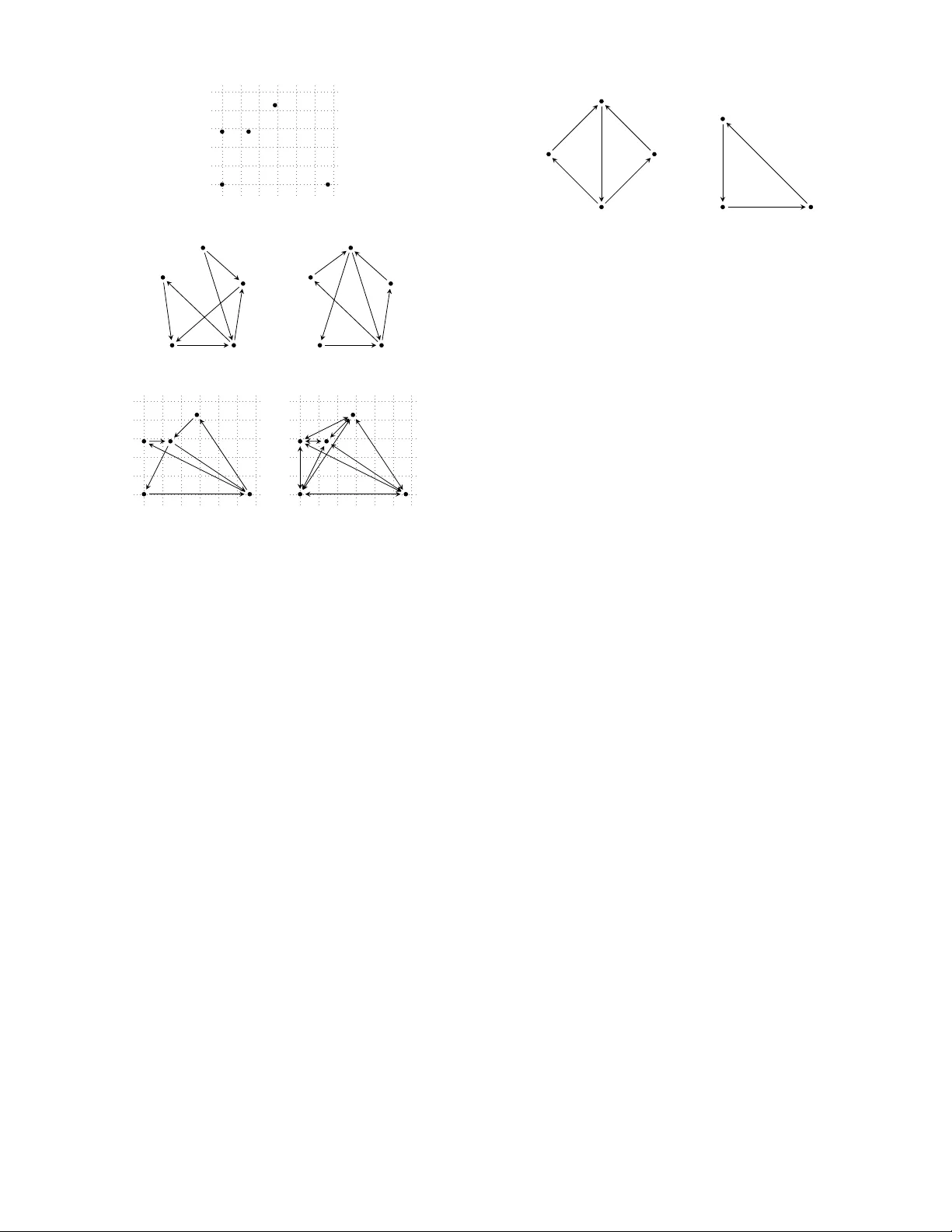
Mathematical aspects of decentralized contr ol of f ormations in the plane M.-A. Belabbas Abstract — In fo rmation control, an ensemble of autonomous agents is required to stabilize at a given configuration i n the plane, doing so whil e agents are a llowed to observ e only a subset o f the ensemble. As such , f ormation control pro vides a rich class of problems for decentralized control methods and techniques. Additionally , it can be used to model a wid e variety of scenarios where decentralization i s a main characteristic. W e introduce here some mathematical background necessary to address questions of stability in decentralized contr ol in general and f ormation co ntrol in particular . This backgr ound in cludes an extension of the notion of global stability to systems evolving on manifolds and a n otion of ro bustness of feedback control fo r n onlinear systems. W e then forma lly introduce the class of fo rmation control problems, and summarize known results. I . I N T R O D U C T I O N W e present h ere some con cepts and definitions re lated to the study of decen tralized and multi-a gent systems in gen eral and to formatio n con trol in particular . W e start with the in troductio n of typ e-A sta bility . It h as been known since at least Poincar ´ e that the topo logy of the manifold on which a system evolves strongly affects the typ e of dynam ics that are possible. I n par ticular, glob al stability as it is defined fo r systems on vector spac es is often trivially impo ssible when the manifold is not a vector spac e. W e propose here a definition that is meaning ful for systems ev olv ing o n manif old an d captures the pr actical benefits of global stabilization. The second definition is the one o f r obustness . When solving a control design pr oblem, one is faced with fin ding a c ontrol u ∗ , belonging to admissible set of control U , that achieves a given objecti ve, e.g. stabilization ar ound a g iv en configur ation. In real-world applications, one is of course often confron ted to errors in modelling, noise in the inputs or in the o bservations, or other source s o f u ncertainty that may make a control la w de signed f or an ideal situation f ail. W e intro duce belo w a notion of robustness, akin to the one of linear systems theo ry , that allows us to hand le such situatio n. The intr oduction of robustness comes with an unexpected benefit: a simp lification o f the design prob lem. Ind eed, if there exist a c ontrol law that achieves a given objecti ve non-r obustly , this control would be quite difficult to find. In practical terms, r obustness allows us to confine o ur search to the jet-space of lowest possible o rder [1] ( we give a brief introdu ction to jet spac es in the appendix) . In Section IV, we formally introduce the class of formation control problem s. Our ap proach , which puts at the center config urations of points , and allows u s to under stand the M.-A. Belabb as is with the School of Engineering and Applied Scien ces, Harva rd Univ ersity , Cambridge , MA 02138 belabbas@seas .harvard.edu role o f rigidity theor y as a way to decentr alize the global objective : in the langua ge of the companion paper [2], rigidity has to do with the δ function s, and using it to define the inform ation flow is thus in many ways unn atural. W e c onclude by summ arizing what is known about for ma- tion co ntrol and ab out th e so-called 2-cycles f ormation [3] , [4]. W e mentioned in [2] that a ma jor issue in de centraliza- tion is the existence of n ontrivial loop s of inform ation—that is loop of inform ations tha t the system cannot by-pass. The 2-cycles is the simplest fo rmation that exhibits two nontrivial loops in its information flow graph. These inf ormation loops are th e main sourc e o f d ifficulty in the analysis of th e system [4]. I I . T Y P E - A S TA B I L I T Y Many natu ral an d engineerin g systems are d escribed by a differential equation ev olv ing o n a m anifold M , by op- position to a flat space or vecto r space. For example, the orientation of a rigid bo dy in sp ace is described by a poin t in the Lie group S O (3) [5]; ano ther examp le arise in f ormation control: we have shown [ 6] that, due to the in variance o f the system un der rotatio ns and tr anslations, the state-space of n auton omou s agents in th e plane is given by the man ifold C P ( n − 2) × (0 , ∞ ) . When th e system e volves on a man ifold, glob al no tions such as global stabilization need to be adjusted to remain relev an t. T his is the issue addressed by type-A stability . Consider the control system ˙ x = f ( x, u ( x )) (1) where x ∈ M , a smoo th ma nifold, and all function s a re assumed smooth. According to elemen tary results in Mo rse theory [7], if the manifold M possesses non-tr ivial homolo gy grou ps [8], the system (1) cannot b e g lobally stable in th e usual sense: there is no continu ous u suc h that (1) has a unique equilibrium. From a practical standp oint, howev er , if one could make one equilibrium stable, and all other equilibria either saddles or unstable, the system wou ld behave as if it were glo bally stable. Ind eed, a v an ishingly small pertur bation w ould ensure that the system, if at a saddle or unstable equilibrium, ev o lves to the u nique stable equilibr ium. W e form alize an d elaborate on this observation. Let E d be a finite subset o f M con taining co nfiguratio ns that we would like to stabilize via f eedback . W e are thus interested in the design of a smooth feedback contro l u ( x ) that will stab ilize the system to any po int x 0 ∈ E d . W e call these points the design tar gets or design equilibria : E d = { x 0 ∈ M s.t. x 0 is a design equilibrium } Let E = { x 0 ∈ M s.t. f ( x 0 , u ( x 0 )) = 0 } , the set of equilibria of (1). W e assume that E is finite. As explained above, when the system evolves on a non- trivial manif old, the Morse in equalities m ake it unreason able to expect th at there exists a control u ( x ) th at makes the design equilibria the only equilibria of the system, i.e. a control such that E d = E . W e call the addition al equ ilibria, that are introduced by the non-trivial topolo gy o f the spac e, ancillary equilibria : E a = E − E d . Let us assume for the tim e being that the lin earization of the system at a n equilibr ium has no eigen values with zero real part. W e decomp ose the set E into stable equilibria, by which we mean equ ilibria such th at all the e igen va lues o f the linear ized system have a negativ e real part, and unstable equilibria , where at least o ne eigen valu e of the linearization has a po siti ve real p art. Ob serve that u nder th is definition , saddle points are considered unstable. In summary: E = E s ∪ E u where E s = { x 0 ∈ E | x 0 is stable } and E u = { x 0 ∈ E | x 0 is unstable } . W ith these notions in min d, we intro duce the following definition: Definition 1. Consider the smooth contr ol system ˙ x = f ( x, u ( x )) wher e x ∈ M and the set E of equilibria o f th e system is fi nite. Let E d ⊂ M be a fin ite set. W e say tha t E d is 1) feasible if we can choo se a smooth u ( x ) such that E d ∩ E 6 = ∅ . 2) type- A stable if we ca n choo se a smooth u ( x ) such th at E s ⊂ E d . 3) strong ly typ e-A stable if we can choose a smooth u ( x ) such that E s = E d . When the set E d is clea r fr o m the co ntext, we say that the system is feasible or type-A stable. This definition extends trivially to systems depen ding on a par ameter . The set E d is feasible if we can ch oose u ( x ) such that at least on e equilibrium of the system is a desig n target. It is said to b e type-A stab le if the system stabilizes to E d with prob ability one fo r any r andom ly chosen initial condition s on M . It is str ong ly type-A stable if it is type-A stable an d mo reover all eleme nts o f E d are stable equilibr ia. The usual n otion o f g lobal stability is a par ticular instanc e of type-A stability; indeed, it co rrespon ds to having u ( x ) such that E d = E = E s . Lookin g at the c ontrapo siti ve of this d efinition, a system is n ot type-A stab le if there exists a set of in itial con di- tions, o f strictly positi ve measure, tha t lead to an a ncillary equilibriu m. W e obser ve that type-A stability is a glob al stability notion; in particular , if one ca n choose u such that all design equ ilibria are locally stable, but if this choice forces the appearance of other , undesired equilibria which are also locally stable, the system is n ot type-A stable. The e xample below illustrate th ese notions. Example 1. Conside r a system ˙ x = x (1 − k x 2 ) wher e k ∈ R is a feedback parameter to be chosen by the user . W e show that any E d ⊂ (0 , ∞ ) is n ot typ e-A sta ble. W e first observe that the system has an equilibrium at 0 a nd two eq uilibria at x = ± p 1 /k if k > 0 . The system is thus feasible for any E d ⊂ R . The J a cobian of the system is 1 at x = 0 an d − 2 a t x = ± p 1 /k . F or k > 0 , the ab ove says that E = { 0 , ± p 1 /k } = { p 1 /k } | {z } E d ∪ { 0 , − p 1 /k } | {z } E a . F r om the linea rization of the system, we have that E s = {± p 1 /k } and E u = { 0 } . W e conclude that E s * E d and the system is not type-A stable. I I I . R O B U S T N E S S W e intro duce here a definition of robustness fo r nonlinear systems. W e start by discussing the well-established concept of generic elements, o n which our d efinition of r obustness is based. Inform ally speaking, a property of ele ments of a to polog- ical space is said to be generic if it is shared by almost all elements of the set. Definition 2. A p r operty P is generic for a topo logical space S if it is true on an everywher e d ense intersection o f open sets of S . Everywhere dense intersections of open sets are sometimes called r e sidual sets [9]. In g eneral, asking for a given proper ty to b e generic is a rather strong requ irement, an d oftentimes it is eno ugh to show that a given property is true on an o pen set of para meters, in itial condition s, etc. W e define Definition 3. An element u of a top ological space S satisfies the pr op erty P ro bustly if P is true fo r a ll u ′ in a neigh - borhoo d of u in S . A pr o perty P is r obust if there exists a r obust u whic h satisfies the pr ope rty . In practical terms, if a pr operty satisfied only at non- r obust u ’ s, then it will likely f ail to be satisfied under th e slightest error in modelling or measurement. Remark 1. W e emphasize that when we s eek a r obust contr ol law u ( x ) for stabilization, we seek a con tr ol law such th at the equilibrium that is to be stab ilized r emains stable und er small perturbation s in u ( x ) . The equilibrium, however , may move in the state space. F or example, assume th at the system ˙ x = u ( x ) has the o rigin as a stable equilib rium. If for all g ( x ) in an appr o priate set of perturbations, the system ˙ x = u ( x ) + εg ( x ) has a stable eq uilibrium at a point z ( ε ) near the origin, then th e con tr ol la w u ( x ) is r obust. If, on the contrary , the equilibrium disap pears or b ecomes unstab le, then u ( x ) is not r obust. If ⌉P , the negation of P , is g eneric, then th ere is n o robust u tha t satisfies P . I ndeed, if ⌉P is generic, then P is verified on at mo st a nowhere de nse closed set. In particular, P is no t verified on a n open set. The main too l to hand le genericity are jet spaces an d Thom transversality theorem. W e will use the r esults in some parts b elow an d r efer the read er to the append ix and to [1] fo r more information. I V . F O R M AT I O N C O N T RO L W e presen t here the class of f ormation contro l problems in the plane. This class provides a rich set o f examples and models for decentralized control. W e begin with some pr eliminaries. W e call a con figuration of n points in the plan e an equiv alen ce class, und er rota tion and translation, of n p oints in R 2 , see Figur e 1 fo r an example. W e h av e shown in [6] that the space of such normalized equ iv alence classes was a comp lex p rojective space. Let G = ( V , E ) b e a graph with n vertices — that is V = { x 1 , x 2 , . . . , x n } is an ord ered set of vertices and E ⊂ V × V is a set o f edges. T he graph is said to be dir ected if ( i, j ) ∈ E does not imply that ( j, i ) ∈ E . W e let | E | = m be the cardinality of E . W e call the outvalence of a vertex the number o f edg es originating f rom this vertex and the in valence the number of incoming edges. A. Rig idity W e b riefly cover the fun damentals of r igidity and estab lish the relev ant n otation. W e refer the read er to [6], [10] for a more detailed presentation. W e c all a fr amework an embed- ding of a graph in R 2 endowed with the u sual Euclidean distance, i.e. given G = ( V , E ) , a framework p attached to a graph G is a mapping p : V → R 2 . By ab use of notation, we write x i for p ( x i ) . W e define the distance function δ of a framework with n vertices as δ ( p ) : R 2 n → R n ( n − 1) / 2 + : ( x 1 , . . . , x n ) → 1 2  k x 1 − x 2 k 2 , . . . , k x 1 − x n k 2 , k x 2 − x 3 k 2 , . . . , k x n − 1 − x n k 2  , where R + = [0 , ∞ ) . W e denote by δ ( p ) | E the restriction of the range of δ to edges in E . For a graph G with m ed ges, we define L =  d = ( d 1 , . . . , d m ) ∈ R m + for which ∃ p with δ ( p ( V )) | E = d } , where the sq uare root of d is taken entry-wise. Properties of this set an d its r elations to th e number of ancillary equilibria are discussed in [10], [6]. The rigidity matrix of the fram ew o rk is th e Jacobian ∂ δ ∂ x restricted to the edges in E . W e denote it by ∂ δ ∂ x | E . Definition 4 (Rigidity) . 1) A framework is said to be in- finitesimally rigid if th er e are no van ishingly small motions of the vertices, except for r o tations an d trans- lations, that keep th e edge-length con straints on the framework satisfied. This translates into [11] rank( ∂ δ ∂ x | E ) = 2 n − 3 . 2) A fr amework attached to a graph G is said to be r igid if ther e a r e no motions of the vertices that keep the edge lengths constraints satisfied and m inimally rig id if all the edges of the graph are necessary for rigid ity . B. F ormation contr ol: definitio n and open p r oblems W e present here the definitio n of formation control prob- lems. W e b uild the problem ar ound configur ations of points in the p lane, by opp osition to distances between vertices; this allows us to understand the r ole of r igidity in formation control as a to ol to ad dress the distribution of the glob al objective or—with the notation of the companion paper [2]— as a to ol to determ ine which δ i are sufficient. Th is p oint of view also makes clear that there is no reason to assume that th e functions h i describing the info rmation flow should be giv en by a rigid graph. In fact, this overload of G in formation control is a limiting factor as is illustrate d in Section V. W e let x ∈ R 2 n contain the position s of all the ag ents in the for mation and consider gen eral dynamical models of the form. ˙ x = n X i =1 n i X j =1 u ij ( δ i ( µ ); h i ( x )) g ij ( x ) , (2) where u ij is a rea l f unction , g ij are smooth vecto r fields and δ, h are smo oth vector valued functions. W e analyzed th is model in detail in the companio n pap er [2] 1) Con figurations o f n-points: The objective in for mation control is a parametric one. Let P be th e space of co n- figuration s of n po ints in R 2 , up to rig id tran sformatio ns of th e p lane: i.e . a po int in P is an equiv a lence class of points in R 2 n . For o ur p urpo se here, it is enough to describe a configur ation of n p oints in the place by an element of R 2 n − 1 , wh ere we use the translational degree of freedom to set the first point at the o rigin in R 2 . W e represent a design formation by a vector µ ∈ R 2( n − 1) = [ ¯ x 2 , . . . , ¯ x n ] , ¯ x i ∈ R 2 as illustrated in in Figure 1. The vector µ is thus a represen- tati ve of the equi valence class of poin ts obta ined via rotation x 1 x 2 x 4 x 3 x 5 x 6 x 7 x 8 ¯ x 1 ¯ x 2 ¯ x 4 ¯ x 3 ¯ x 5 ¯ x 6 ¯ x 7 ¯ x 8 O Fig. 1: Configur ations of n po ints in the p lane, up to translations, can be represented by a c onfigur ation with x 1 at th e orig in. W e use the n otation ¯ x i for th e coo rdinates of the points after translation. of the ¯ x i . In order to represent the decentralized structure of a forma- tion contro l problem , we introduce two gra phs: the δ - graph and the h -g raph, rep resenting resp ectiv ely the informatio n a giv en agen t has ab out the global ob jectiv e of the form ation ( δ -g raph) and about the state o f the formation ( h -gra ph). In mor e detail, to each agent with position x i ∈ R 2 we associate a vertex i in V . W e let G be a graph with vertex set V and set of edges E . The ed ges de fine th e dece ntralized structure as f ollows: assume that vertex i has outvalence k and the edges ( i, l 1 ) , . . . , ( i, l k ) ∈ E h are leaving from vertex i . The h -graph G h = ( V , E h ) defines the functions h i ( x ) accordin g to: 1: Rang e only informa tion: in this case, a n agent is only able to measure its distance to its various neig hbors. h R i ( x ) : R 2 n → R k : x → ( k x l 1 − x i k , . . . , k x l k − x i k ) . 2: Relative position in formatio n: in this case, agen t i can measure the r elative positions o f its neighb ors . Using some simp le trigon ometric rules, it is easy to see that in orde r to reconstru ct the relative positions of its neig h- bors (i.e. their position relativ e to x i , up to rotation), it is sufficient for agent i to have the distances to the agents as well as the inner p roduc ts ( x l 1 − x i ) T ( x l j − x i ) , j = 2 . . . k . W e have h i ( x ) = ( h R i ( x ) , ( x l 1 − x i ) T ( x l 2 − x i ) T , . . . , ( x l k − x i ) T ( x l 1 − x i )) . A formation is an ensemb le of agen ts to gether with an h - graph. Remark 2. The h-graph , which is pr oper to formatio n contr ol, is r elated to the information flow graph defined [2]. The fun ction δ i are similarly described by a g raph G δ = ( V , E δ ) . Assume th at vertex i has outvalence k and the e dges ( i, l 1 ) , . . . , ( i, l k ) ∈ E δ are lea ving from vertex i . W e have 1: Rang e on ly in formation : an agent only kn ows abou t the distance at which it needs to stabilize from its neighbors. δ i ( µ ) = ( k ¯ x l 1 − ¯ x i k 2 , . . . , k ¯ x l k − ¯ x i k 2 ) . 2: Rang e an d an gle: in this case, th e age nts also k nows the relativ e position at wh ich its ne ighbor s ar e in th e target framework: δ i ( µ ) = ( δ R i ( µ ) , ( ¯ x l 1 − ¯ x i ) T ( ¯ x l 2 − ¯ x i ) T , . . . , ( ¯ x l k − ¯ x i ) T ( ¯ x l 1 − ¯ x i )) . Example 2. Consider a forma tion contr o l pr oble m wher e we r equ ir e th e agents to stabilize at the config uration of points described in F igure 2 a. The h -graph of F igu r e 2b corr espon ds to the observatio n functions, assuming the r elative po sition case: h 1 ( x ) = k x 2 − x 1 k h 2 ( x ) =  k x 3 − x 2 k , k x 4 − x 2 k , ( x 3 − x 2 ) T ( x 4 − x 2 )  h 3 ( x ) = k x 3 − x 1 k h 4 ( x ) = k x 4 − x 1 k h 5 ( x ) =  k x 2 − x 5 k , k x 3 − x 5 k , ( x 2 − x 5 ) T ( x 3 − x 5 )  . Similarly , the h -graph of Figur e 2c corr espo nds to h 1 ( x ) = k x 2 − x 1 k h 2 ( x ) =  k x 3 − x 2 k , k x 4 − x 2 k , ( x 3 − x 2 ) T ( x 4 − x 2 )  h 3 ( x ) = k x 3 − x 5 k h 4 ( x ) = k x 4 − x 5 k h 5 ( x ) =  k x 2 − x 5 k , k x 1 − x 5 k , ( x 1 − x 5 ) T ( x 2 − x 5 )  . The δ -g raph of F igu r e 2d corr espo nds to the fun ctions δ i given by δ 1 ( µ ) = k ¯ x 2 − ¯ x 1 k δ 2 ( µ ) = ( k ¯ x 3 − ¯ x 2 k , k ¯ x 4 − ¯ x 2 k ) δ 3 ( µ ) = k ¯ x 3 − ¯ x 5 k δ 4 ( µ ) = k ¯ x 4 − ¯ x 5 k δ 5 ( µ ) = ( k ¯ x 2 − ¯ x 5 k , k ¯ x 1 − ¯ x 5 k ) in the c ase o f distance on ly informatio n. In the c ase of r elative position information, δ 2 and δ 4 would a lso con tain the in ner p r oducts o f the a ppr op riate ¯ x i . The δ -graph of F ig- ur e 2e corr esp onds to letting every agent know its distance to a ll othe r agents in th e ca se of range on ly information , and letting δ i ( µ ) = µ for all i in the case o f r elative p osition. Formation control problems are co ncerned with stabiliza- tion, either local o r type-A. T wo different fla vors h av e b een studied in the literature: 1) Stabilize at a given fra mework : the glo bal o bjective is described as the stabilization at the framework descr ibed by µ . I n this case, the card inality of E d , the set of design equilibria, is one (up to mirro r symme try). Rigidity theory tells us that G δ needs to be globally rigid [6]. ¯ x 1 ¯ x 2 ¯ x 4 ¯ x 3 ¯ x 5 (a) x 1 x 2 x 4 x 3 x 5 (b) x 1 x 2 x 4 x 3 x 5 (c) x 1 x 2 x 4 x 3 x 5 (d) x 1 x 2 x 4 x 3 x 5 (e) Fig. 2: W e rep resent in ( a ) a configur ation of 5 po ints in the plane. Figures ( b ) and ( c ) repr esent two possible h - graph f or a formatio n control pro blem. Figur es ( d ) and ( e ) two po ssible δ - graph . Observe that the δ graph of Figure ( e ) is fully con nected, h ence ev ery agent knows the globa l objective. 2) Stabilize at one of many fra mework : Gi ven a con figu- ration of n -points ( n ≥ 4 ) µ , let G δ be a minimally rigid graph . Th e objective is to stabilize at any frameworks such that the edge lengths in G δ are satisfied. Because the graph is m inimally rigid —and not globally rigid— there are several fra mew orks which have the same edge lengths f or ed ges o f G δ (see Figure 5 for an example, or in Fig ure 2d, tak ing the mir ror symmetric of ¯ x 1 with respect to the ¯ x 2 − ¯ x 5 axis yields a f ramework with similar edge leng ths). In this ca se, E d is gi ven by all frameworks which satisfy the given ed ge lengths and the δ i ’ s are of the range only type. W e re visit these ideas in Section V. W e conclu de this section by m entioning b road open qu estions in f ormation control: 1) How many frameworks satisfy a gi ven set of edge lengths? W e ha ve given a lower bou nd in a p articular case in [6], but th e general case is not settled. 2) How sparse can the gra phs G δ and G h be in or der to guaran tee the existence of robust u i ( δ i ; h i ) that yield type-A stabilization? 3) How sparse can the gra phs G δ and G h be in or der to guaran tee the existence of robust u i ( δ i ; h i ) that yield have local stabilization aroun d any po int in E d ? x 1 x 2 x 3 x 4 (a) The tw o-cyles formation x 1 x 2 x 3 (b) The triangle forma- tion Fig. 3 While rigidity theory clearly has a r ole to p lay in a complete u nderstand ing of th e δ -graph , it is not clear that it will have m ore than a supporting role for investigations related to the h -graph . In the case of the δ -g raph, a first obvio us result is that minimal rigidity (and Laman theorem [6]) yields a ”minimal” undirected δ -gra ph: a le ss dense graph is not giving agents enoug h about the glob al objective to allo w them to satisfy it. The case of directed formation is already much mo re complex. W e p rovide pa rtial an swers to th ese que stion in Section V. V . T H E T W O - C Y C L E S F O R M AT I O N A N D OT H E R K N O W N R E S U LT S W e p resent som e known results in form ation control an d illustrate in this section the notions intr oduced in this paper on the 2-cycles formatio n, which was exhibited in [4] as an example of the difficulty to make prog ress in formatio n control when there are ”loops of in formatio n” in the system. It was co njectured [12] that for mation co ntrol problems whose objective is minimally rigid, and whose under lying δ -gr aph (the h -graph was assumed to be the same as the δ - graph) has no vertices with outvalence larger that two we re globally (or type-A) stabilizable. Sin ce then, we h ave shown it was not the case for the 2-cycles. The tw o-cycles is the formation rep resented in Figure 3a. Let x i ∈ R 2 , i = 1 . . . 4 represen t the position of the 4 agents in the plane. W e define the vectors            z 1 = x 2 − x 1 z 2 = x 3 − x 2 z 3 = x 1 − x 3 z 4 = x 3 − x 4 z 5 = x 4 − x 1 (3) Hence, the observation fu nction are gi ven b y h 1 ( x ) = ( k z 1 k , k z 5 k , z T 1 z 5 ) , h 2 ( x ) = k z 2 k , h 3 ( x ) = k z 3 k , h 4 ( x ) = k z 4 k . (4) W ith th e n otation of Figure 4 , we let µ = [ ¯ x 2 , ¯ x 3 , ¯ x 4 ] parametrize a configu ration of f our points in th e plan e. W e let k ¯ x 2 k = d 1 , k ¯ x 4 k = d 5 , k ¯ x 3 − ¯ x 2 k = d 2 , etc. W e take the δ -g raph to b e the same as the h -grap h and consider the range only case. Hence, the functions δ i are gi ven by δ 1 ( µ ) = ( d 1 , d 5 ) , δ 2 ( µ ) = d 2 , δ 3 ( µ ) = d 3 , δ 4 ( µ ) = d 5 , (5) ¯ x 1 ¯ x 2 ¯ x 3 ¯ x 4 d 1 d 5 d 2 d 4 d 3 Fig. 4: Any fr amew ork in the plane with ¯ x 1 6 = ¯ x 2 is congru ent to a framework with ¯ x 1 = (0 , 0) and ¯ x 2 on the x -axis It is con venient to intr oduce variables fo r the error in edge lengths: e i = z T i z i − d i . The set of vector fields that respect both th e in variance of the system u nder the S E (2) action as presented in [6] is giv en by Hence a general control law fo r such a system is            ˙ x 1 = u 11 ( δ 1 ( µ ); h 1 ( x )) g 11 ( x ) + u 12 ( δ 1 ( µ ); h 1 ( x )) g 12 ( x ) ˙ x 2 = u 2 ( δ 2 ( µ ); h 2 ( x )) g 2 ( x ) ˙ x 3 = u 3 ( δ 3 ( µ ); h 3 ( x )) g 3 ( x ) ˙ x 4 = u 4 ( δ 4 ( µ ); h 4 ( x )) g 4 ( x ) (6) with g 11 ( x ) = ( x 2 − x 1 ); g 12 ( x ) = ( x 4 − x 1 ); g 2 ( x ) = x 3 − x 2 ; g 3 ( x ) = x 1 − x 3 and g 4 ( x ) = x 3 − x 4 . W e d enote by F the space of control systems of the type of Equatio n (6), with the u i smooth real-valued functions of their argument. W e equip F with the C r topolog y . x 1 x 2 x 3 x 4 (a) x 1 x 2 x 3 x 4 (b) x 1 x 2 x 3 x 4 (c) x 1 x 2 x 3 x 4 (d) Fig. 5: Four framew orks in the plane that are not equiv alent under rotations and translation and that ha ve the same corresponding edge lengths. ( a ) is the mirror-symmetric of ( c ) and ( b ) is the mirror- symmetric of ( d ) . The set o f design equilibr ia E d for the 2-cycles is of cardinality 4, u p to rig id transfo rmations, since th ere are fo ur frameworks in the plane for which e i = 0 ; they are depicted in Figure 5. Hence, the global objective 1 can be written as an equality objective with F ( µ ; x ) =       k x 2 − x 1 k 2 − d 1 k x 3 − x 2 k 2 − d 2 k x 1 − x 3 k 2 − d 3 k x 3 − x 4 k 2 − d 4 k x 1 − x 4 k 2 − d 5       with the add itional require ment of eith er stabilizing locally any of these equilibria or seeking a con trol such that the system is type-A stable. The lo cal o bjectives 2 for each agents ar e to stabilize at the required distance f rom their n eighbo rs. For agent 1, we have f 1 ( δ 1 ( µ ); h 1 ( x )) =  k x 2 − x 1 k 2 − d 1 k x 4 − x 2 k 2 − d 5  , and for agents i = 2 , 3 , 4 : f 2 ( δ 2 ( µ ); h 2 ( x )) = k x 3 − x 2 k 2 − d 2 f 3 ( δ 3 ( µ ); h 3 ( x )) = k x 1 − x 3 k 2 − d 3 f 4 ( δ 4 ( µ ); h 4 ( x )) = k x 3 − x 4 k 2 − d 4 Satisfying the local objectives clearly imp lies that the global objective is satisfied. In general, the set E a of ancillary equilib ria depends on the choice of feedbacks u i . Due to the in variance and d istributed nature of th e system, we ca n exhibit some con figuration s that belong to E a for all u i ’ s. [10]: Proposition 1. The set E contain s, in add ition to the equi- libria in E d , the frame works characterized by 1) z i = 0 fo r all i , which co rr espo nds to having all the agents sup erposed. 2) all z i ar e alig ned, which corr e sponds to havin g all agents on the same one-d imensiona l subspace in R 2 . These fr ameworks form a thr ee dimen sional invariant subspace of the dynamics. 3) e 2 = e 3 = e 4 = 0 , z 1 and z 5 ar e align ed and so that u 1 ( δ 1 ; h 1 ) k z 1 k = ± u 5 ( δ 1 ; h 1 ) k z 5 k , wher e the sign d epends on whethe r z 1 and z 5 point in the same or opposite dir e ctions. As we have discussed in the comp anion p aper [2], the δ i giv en in Equatio n (5) do no t saturate the o bservation function s. Hence there may be some gain in letting δ be more informative. W e know that a max imally infor mative δ i would be given b y the id entity fun ction. This maximally informa ti ve δ i was used in [1 3] to prove that the 2 -cycles can be locally stabilized at a giv en f ramework in the plane using a r elativ ely simple control law an d adju sting some feedback gains. The dy namics used was of the typ e of Eq uation 6 with the contro l law u i = k i e i , i = 1 , . . . , 5 (7) 1 The global objec ti ve of a decent ralize d system, de fined in [2], is ac hie ved at configurations x such that F ( µ ; x ) = 0 . 2 Local objecti ves, also defined in [2], are achi e ved by an agent at configurat ions such that f i ( δ i ( µ ); h i ( x )) = 0 . where the k i are constant real-valued gain s used by th e agents to locally stabilize a gi ven framew ork ( i.e. k i = k i ( µ ) ). W e can restate th e theorem in the lan guage of this paper as follows: let E 4 be the space of a ll configura tions o f 4 points in the plane. Theorem 1 ( Reformulatio n o f [13]) . If we let δ i ( µ ) = µ for all i and h i as in Eq uation (4) , th er e e xists u i ( µ ; h i ( x )) such that for all µ , the framework parametrized b y µ is loca lly stable for the system of Equ ation (6) with c ontr ols u i . In fact, a con tr ol law o f th e type of Equa tion (7) works for config urations of n points in R n , with h -g raph given b y a minimally rigid graph with o utvalence at each node a t most two (and δ i being maximally informative). Sketch o f pr oof. The proo f relies on the linearizatio n of the system aroun d a gi ven f ramework. It is then showed that by mu ltiplying th e Jacobian o f the system b y a b lock diagona l matrix—cor respond ing to th e g ains—one can make all e igenv alues o f th e pr oduct h av e n egati ve real pa rt. T o this end, a result similar to the one in [ ? ] is proved for the case of real matrices.  W e h av e shown in [1] that th e same result does not ho ld if we let the δ -grap h be th e same as the h -graph: Theorem 2. Given δ i ( µ ) as in Equatio n ( 5) and h i as in Equation ( 4) , there ar e no robust contr o l system in F that locally stabilize all frameworks in E 4 . In fact, for any u i ∈ U i , there exist s a set of frameworks of positive measur e in E 4 that ar e not locally stabilizable. Sketch o f pr oof. The proof relies o n showing that, given the δ i and h i , satisfying the local objectives ro bustly prevents the global stabilization objective to be satisfied.  Local stabilization of formation s with e ither symme tric or cycle-free h - an d δ -gr aph, is muc h easier to ha ndle. W e mention here that linear decentralized co ntr ol pr oblem whose informa tion flo w was giv en by a gr aph without cycles have been stud ied in [ 14]. W e cite the following result from formation con trol, which relies on similar graphs in th e directed case: Theorem 3 (Loc al stabilization of bi-d irectional forma- tions [15]) . Given a con figuration of n points in th e pla ne with δ -graph G = ( V , E ) that is infinitesimally rigid , a nd h -graph equal to δ - graph, the c ontr ol law u i ( δ i ( µ ) , h i ( x )) = X j s.t. ( i,j ) ∈ E ( k x i − x j k − d k )( x i − x j ) locally stabilizes almost all infi nitesimally rigid frame works. The same h olds true for directed f ormation s , where the δ - and h - gr aphs are the same and contain no loops an d every vertex h as outvalen ce of two at the most. Sketch o f pr oof. The proof is based on a linearization of the system about an equilibriu m.  For a description of the co nfigura tions that are excluded by the qualifier ”almost all”, we refer the reader to [15]. Results abou t global stabilization of for mations, whether directed o r und irected, are much mor e sparse. W e mention the result of [16] about the triangular formation : Theorem 4 (T y pe-A stab ility of triangular formation. [1 6]) . Consider the triangular fo rmation of F igur e 3b. The con tr ol law ˙ x i = ( k x i +1 − x i k − d i )( x i +1 − x i ) makes the system r obustly type-A stable for almost a ll config urations of points in E 3 Sketch o f pr oof. The proof is based on exhibiting a L yapun ov-like [ 4] func tion for the system and showing that, except for what is called a ”thin set” of initial conditions (i.e. a set of codime nsion on e), th e system is globa lly stable. This can be rephr ased using th e type-A stability idea as we have don e h ere.  Even more, type-A stability was shown, using a similar L yapun ov argument, for a broad class of decentralized con- trol law in [4]. W e have shown t hat this result does not extend to the 2-cycles: Theorem 5. Ther e ar e no r o bust u ∈ U with δ i as in Equation ( 5) an d h i as in E quation (4) su ch that th e 2 -cycles formation is type-A stable. Sketch o f pr oof. The theory of bifu rcation and singula rities was used to show that the d ecentralized structure of the system forces the app earance of stable, anc illary eq uilibria for all feedback laws u ∈ U .  Whether lettin g δ i to be the identity would allow to find a robust, typ e-A stabilizing co ntrol for the two-cycles is an open question. V I . S U M M A RY W e have de fined formation control problems in the plane and introdu ced so me relev ant m athematical concep ts: typ e- A stability and ro bustness. The presen tation of formation control h ighlighted the difference between the d ecentraliza- tion o f th e system as it is com monly und erstood (agents have a par tial inform ation about the state of th e ensemble) and the decentralization of the objective ( agents ha ve a partial informatio n ab out what co nfiguratio n th e formation is asked to reach) . W e have seen that the latter type of decentralizatio n, though no t often acknowledged, affects the behavior o f formations gr eatly ( compar e Th eorems 1 and 2). Finally , we have presented som e open qu estions in fo rmation control. A P P E N D I X The main to ol for h andling gen ericity and robustness in function spaces is Thom ’ s transversality theore m. W e will arrive at the result by building on to the simpler concep t of transversality of lin ear subspaces. Thom’ s theo rem rou ghly answers th e following typ e of questions: g iv en a fu nction u from a manifold M to a manifold N , and some relations between the de riv atives of x y = u ( x ) u ( x ) ˜ u ( x ) ˜ ˜ u ( x ) Fig. 6: If we let P be the p roperty o f v an ishing with a zero deriv ati ve. W e will prove in this section that ⌉ P is generic and thus P is not r obust. Let u ( x ) be a function which satisfy P . For any small pertu rbations, it will eith er vanish with a non -zero deriv ativ e—as illustrated with ˜ u ( x ) , dashed curve— o r no t v anish at all—as illustrated with ˜ ˜ u ( x ) , d otted curve. Both ˜ u ( x ) and ˜ ˜ u ( x ) are transversal to the m anifold defined by y = 0 e verywhere, wh ereas u ( x ) is not. different o rders of this function (e.g. u ′′ + u ′ − u = 0 ) , under what c ircumstances are these relatio ns preserved under small p erturba tions of the function ? For example, if a r eal- valued function has a zero at some point, un der a small perturb ation of this function, the zero will persist generically for u . On th e oth er hand, if a real-valued f unction vanishes with its second deriv ati ve also being zero , unde r a small perturb ation this prop erty will be lost, see Figu re 6. Th e crux of T hom’ s theorem is to show tha t considering on ly a “small subset” of pertu rbations (th e in tegrable p erturbatio ns as we will see below) in the set of all p erturba tions in jet-sp aces is sufficient. Let A, B ⊂ R n be linear subspaces. They are transversal if R n = A ⊕ B , where ⊕ denotes the direct sum. For example, a plane and a line not containe d in the p lane are tran sversal in R 3 . The notion of transversality can be exten ded to m aps as follo ws: giv en F 1 : R n → R m and F 2 : R l → R m , we say that F 1 and F 2 are tran sversal at a point ( x 1 , x 2 ) ∈ R n × R l if one of the two follo wing conditions is met: 1) F 1 ( x 1 ) 6 = F 2 ( x 2 ) 2) If F 1 ( x 1 ) = F 2 ( x 2 ) , then the matrix  ∂ F 1 ∂ x ∂ F 2 ∂ x  is o f f ull rank. In particu lar , if l + n < m then F 1 and F 2 are tr ansversal only where they do not map to the same point. This definition extends immediately to smoo th func tions between smooth manifold s: given F 1 : M 1 → N and F 2 : M 2 → N , we say th at F 1 and F 2 are tr ansversal at ( x 1 , x 2 ) ∈ M 1 × M 2 if either F 1 ( x 1 ) 6 = F 2 ( x 2 ) or F ( x 1 ) = F ( x 2 ) and the tangent space of N at F ( x 1 ) is the direct sum of the ima ges of the tangent spaces of M 1 and M 2 under F 1 and F 2 respectively , i.e. T F 1 ( x 1 ) N = F 1 ∗ T x 1 M 1 ⊕ F 2 ∗ T x 2 M 2 where F ∗ is the push-fo rward [8] of F . Example 3. T ake M 1 = R and M 2 = N = R 2 and let F 1 ( x 1 ) = x 1 v + b 1 and F 2 ( x 2 ) = Ax 2 + b 2 , wher e A ∈ R 2 × 2 , b 2 , v , x 2 ∈ R 2 and x ∈ R . If b 1 6 = b 2 , then F 1 (0) 6 = F 2 (0) and F 1 is transversal to F 2 at (0 , 0 , 0) . I f b 1 = b 2 , then F 1 (0) = F 2 (0) and the function s ar e transversal if the span of v and the columns of A is R 2 . The notion of transversality that is of inter est to us is a straightfor ward extension of the transversality o f maps: Definition 5 (T r ansversality) . Let F : M → N be a smooth map and let C be a submanifold of N . Th en F is transversal to C at a given po int if, a t that point, F is transversal to the embedd ing i : C → N of C into N . Example 4. T ake N = R 3 with coordinates u, v , w and C be the u -v plane. Let F : R → R 3 : x → [ x, 2 x, 3 x ] T . Then the map F is transversal to C everywher e. Example 5. Let F ( x ) : R → R 3 be any smooth curve in R 3 and C b e the u -axis. At po ints wher e F ( x ) ∈ C , the tangent vector to C a nd the tan gent ve ctor to F will spa n at most a two-dimension al subspace in R 3 . Hence, F is transversal to C only at the points wher e F ( x ) / ∈ C . A. Jet Spaces Let F, G : M → N be smooth map s between smooth manifold s M an d N endowed with a metric. W e say th at F and G are k- equivalent at x 0 ∈ M if in a neigh borho od of x 0 we have k F ( x ) − G ( x ) k = o ( k x − x 0 k k ) . One can verify [17] that k- equiv alence is independent o f the choice o f metric s on M and N and that it is an equi valence relation on maps. In fact, the above definition can be recast as saying that F and G are 0-equivalent at x 0 if F ( x 0 ) = G ( x 0 ) , 1-equivalent if in addition ∂ F ∂ x | x 0 = ∂ G ∂ x | x 0 , and so for th. W e define the k-jet of a smo oth map to be its k-equivalence class: Definition 6. The k-jet of F : M → N at x 0 is J k x 0 ( F ) = { G : M → N s.t. G is k-equivalent to F } . Hence, th e 0-jet o f F at x 0 is F ( x 0 ) ; the 1 -jet is ( F ( x 0 ) , ∂ F ∂ x | x 0 ) , etc. For example, th e con stant function 0 and sin( x ) have th e same 0-jet at x = 0 a nd x and sin( x ) have the same 1-jet at 0 . W e define: J k ( M , N ) = Space of k- jets from M to N . A 0-jet is th us dete rmined by a po int in M and a po int in N , an d thus J 0 ( M , N ) noth ing mor e than the Cartesian produ ct o f M and N : J 0 ( M , N ) = M × N . Since a 1-jet is d etermined by a pair of points,fo r the 0 - jet part, and a matrix o f dimension dim M × dim N , for the Jacobian of the function at x 0 , we see that dim J 1 ( M , N ) = dim M + dim N + dim M dim N . W e cannot say in general that J 1 ( M , N ) is the cartesian prod uct of J 0 with R m × n since the produ ct may be twisted. Similar r elations are obtained for higher jet-spaces [17] Giv en a functio n F : M → N , we ca ll its k-jet extension the map given by j k F ( x ) : M → J K ( M , N ) : x → ( F ( x ) , ∂ F ∂ x ( x ) , . . . , ∂ k F ∂ x k ( x )) . Example 6. Let M = N = R . The k-jet s pace is J k ( R , R ) = R × R × . . . × R = R k +2 . T ake F ( x ) = sin( x ) ; the 2 − jet extension o f F is j 2 sin ( x ) = ( x, sin( x ) , cos( x ) , − sin( x )) . If we take M = N = R 2 and F ( x ) = Ax for A ∈ R 2 × 2 , then j k Ax ( x ) = ( x, Ax, A, 0 , . . . , 0) . Remark 3. The concepts pr esen ted in this section a lso trivially apply to vector fields on M , by letting N = T M . While to any function F : M → N , we can assign a k-jet extension j k F : M → J k ( M , N ) , the inv erse is not true: th ere are maps G : M → J k ( M , N ) wh ich do not correspo nd to functions from M to N as there are som e obvious integrab ility con ditions that ne ed to b e satisfied. For example, if we let G : R n → J 1 ( R n ) : G ( x ) = ( x, Ax, B ) , then G is a 1-jet e xtension of a function if and only if B = A . The p ower o f the transversality the orem of Tho m is that it allows one to dr aw co nclusions ab out transversality proper- ties in gener al, an d g enericity in p articular, by solely loo king at perturbations in jet spaces that ar e jet extensions —a much smaller set than all perturb ations in jet-spac es, since these include the much larger set o f non-integrab le perturba tions. W e recall that the C r topolog y is a m etric topology . It is induced by a metric that takes in to acco unt the fu nction and its first r deriv a ti ves. W e have: Theorem 6 (Th om’ s transversality) . Let C b e a r egular submanifold of the jet space J k ( M , N ) . Then the set of ma ps f : M → N who se k -jet extensions are transversal to C is an everywher e d ense intersection of o pen sets in the space of smooth maps for the C r topology , 1 ≤ r ≤ ∞ . A typ ical application of the theorem is to pr ove that vector fields with degener ate zeros are not generic. W e here prove a version of th is result that is of interest to us. Corollary 1. Functions in C ∞ ( M ) whose d erivative at a zer o vanish ar e not generic. In o ther words, th e cor ollary deals with the intuitive fact that if u ( x ) = 0 , then generica lly u ′ ( x ) 6 = 0 . This result also goes under the name of weak-transversality theorem [ 18]. Pr oof. Consider th e space of 0-jets J 0 ( M , R ) . I n this space, let C be th e set of 0- jets which vanish, i.e. C = ( x, 0) ⊂ J 0 . A fun ction u is transversal to this set if either it d oes not vanish, or wh ere it v anishes we have that the matrix  1 1 0 ∂ f ∂ x  is of full r ank. Hen ce, tran sversality to C at a z ero im plies that the d eriv ative o f the f unction is non-zer o. The result is thus a consequenc e o f Theorem 6.  T o picture the si tuation geometrically , recall that J 0 ( M , R ) is simp ly M × R . Hence C is M × 0 ⊂ J 0 ( M , R ) . The result says that any fu nction th at intersects C witho ut crossing (and h ence with a ze ro derivati ve) will, u nder a generic perturb ation, either cross C or not intersect C at all, since these two eventualities result in tran sversality . Figur e 6 provides an illustration when M = R . R E F E R E N C E S [1] M.-A. Belabbas, “Decen traliz ed formation control pa rt ii: Alge braic aspects of inf ormation flo w and singulari ties, ” In S ubmission, avail able at arXiv:1101.2421 , 2011. [2] ——, “Kno wn unknown s, unkno wn unkno wns and informat ion flo w: ne w results a nd challenges in decentral ized control, ” in P r oceedings of the 9t h International Confe re nce on Contr ol and Automatio n , 2011. [3] ——, “On global feedback stabilizat ion of decent ralize d formatio n control , ” in T o appear in Pr oceedin gs of 2011 Confere nce on Dec ision and Contr ol , 2011. [4] M. Cao, A. Morse, C. Y u, B. Anderson, and S. Dasgup ta, “Maintai ning a directed, triangular formation of mobile autonomous agents, ” Comm. in Information and Systems , v ol. 11, no. 1, pp. 1–16, 2011. [5] A. Bloch, Nonholonomi c mechanics and cont r ol . Springer , 2003. [6] M.-A. Belab bas, “Geometric properties of formati on cont rol, ” in Submitte d , available on my websi te , 2011. [7] J. Milnor , Morse Theory . Princ eton Uni versity Press, 1963. [8] F . W arner , F oundations of Dif fer entiable Manifolds and Lie G r oups . Springer , 1983. [9] V . I. Arnold, V . Afraimovi ch, Y . Ilyashenk o, an d L. Shilniko v , Bifurca- tion theo ry in Dynamical Systems V . Encyclopae dia of Mathematical Scienc es . Springer , 1994. [10] M.-A. Belabbas, “Dece ntraliz ed formation contro l part i: Geomet ric aspects, ” In Submission, availa ble at arXiv:1101.2416 , 2011. [11] J. E. Graver , B. Serva tius, an d H. Serva tius, Combinatorial Rigidity . Amer . Math. Soc., 1993. [12] M. Cao, A. S. Morse, C. Y u, B. D. O. Ande rson, and S. Dasgupt a, “Control ling a tri angular formation of mobile autonomous agents, ” in Pr oc. of the 46th IEEE Confe ren ce on Dec ision and Contr ol , vol. 46, 2007, pp. 3603–36 08. [13] C. Y u, B. Anderson, S. Dasgupta, and B. Fidan, “Control of minimally persisten t formations in the plane, ” SIAM J ournal on Contr ol and Optimizati on , vol. 48, no. 1, pp. 206– 233, 2009 . [14] P . Shah and P . A. Parrilo, “ A poset frame work to model decen traliz ed control problems, ” in Proc. of the 48th IEEE Confer ence on Decision and Contr ol , vo l. 48, 2009. [15] L. Krick, M. E . Brouck e, and B. Francis, “Stabi lizati on of infin itesi- mally rigid formations of multi-robot networks, ” Interna tional Journal of Contr ol , 2008. [16] B. Anderson, C. Y u, S. Dasgupta, and A. S. Morse, “Control of a three-c oleade r format ion in the plane, ” Systems and contr ol lette rs , vol. 56, pp. 573–578 , 2007. [17] V . Arnold, “Lectures on bifurcatio ns and versal familie s, ” in Russian Math. Survey s , vol. 27, 1972, pp. 54–123. [18] V . Guillemi n and M. Golubitsk y , Sta ble mappings and their singul ar- ities . Spring er , 1974.