Large-Sample Confidence Intervals for the Treatment Difference in a Two-Period Crossover Trial, Utilizing Prior Information

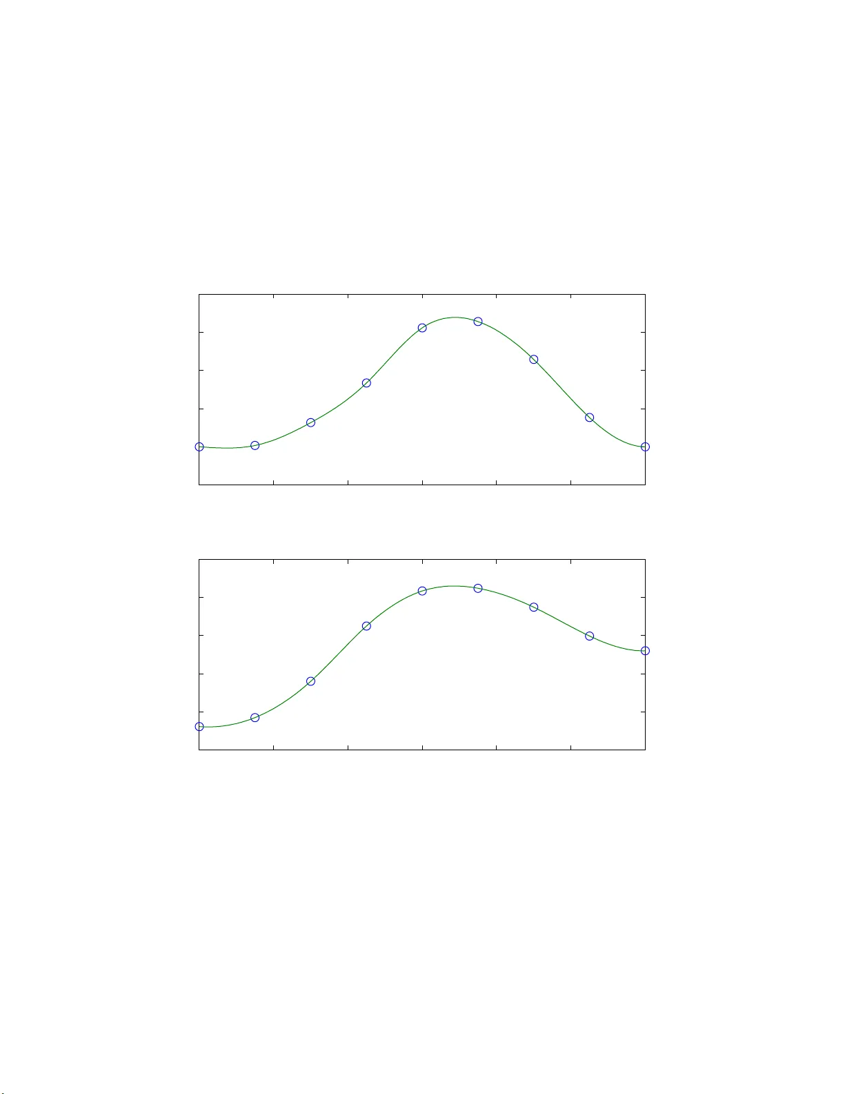
Large-Sample Confide nce In terv als for the T reatmen t D i ffe rence in a Tw o-P erio d Crosso v er T rial, Uti l i zing Prior Infor matio n P aul Kabaila ∗ and Khagesw or G iri Departmen t of Mathematics and Statistics, La T rob e Univ ersit y , Victoria 308 6, Australia Abstract Consider a t w o-treatmen t, t w o-p erio d crosso v er trial, with responses that are con tin uous random v ariables. W e find a la rge-sample frequen tist 1 − α confidence in terv al for the treatmen t difference that utilizes the uncertain prior informatio n that there is no differen tial carryo v er effect. Keywor ds: Differen tial carry o v er effect; Prior information; Tw o-p erio d crossov er trial. ∗ Corresp onding author. Address: Department of Mathematics and Statistics, La T rob e Univ ersit y , Victoria 3086, Australia; T el.: +61- 3-9479- 2594; fax: +61- 3-9479- 2466. E- mail addr ess: P .Kabaila@latro b e.edu.au. 1 1. In tro duction W e consider a t w o-t reatmen t t w o- p erio d crosso v er trial, with resp o nses that are con tin uous random v ariables. This design is very p opular in a wide range of medical and other applications, see e.g. Jones and Ken w ard (1989) and Senn (200 6). The purp ose of this trial is to carry out inference ab out the difference θ in the effects of t w o treatments , lab elled A and B. Sub j ects are randomly allo cated to either group 1 or g roup 2. Sub jects in gro up 1 receiv e treatmen t A in t he first p erio d and t hen receiv e treatmen t B in the second p erio d. Sub jects in group 2 receiv e treatmen t B in the first p erio d a nd then receiv e treatment A in the second p erio d. This design is efficien t under the a ssumption that there is no differen tial carryo v er effect. It is not an appro pria te design unless there is strong prior information that this assump- tion holds. How ev er, a commonly o ccurring scenario is that it is not certain that this assumption holds. W e consider this scenario. T o deal with this uncertain t y , it has b een suggested (starting with G rizzle, 1965, 19 74 and endorsed by Hills and Armitage, 1979) that a preliminary test of the n ull hy p o thesis that this assumption holds b e carr ied out b efore pro ceeding with further inference . If this test leads to acceptance o f this null h yp ot hesis then further inference pro ceeds on the basis that it w as kno wn a priori that t here is no differen tial carry ov er effect. If, on the o ther hand, this null h yp othesis is rejected then furt her inference is based solely on data from t he first p erio d, since this is unaffected b y an y carry ov er effect. In a landmark pap er, F reeman (1989) sho w ed that the use of suc h a preliminary hy p o thesis test prior to the construction of a confidence in terv al with nominal co v erage 1 − α leads to a confidence in terv al with minim um co v erage probability far below 1 − α . F or simplicit y , F reeman supposes that the sub ject v ariance and t he error v ariance are kno wn. In other words, F reeman presen ts a lar g e-sample analysis. F reeman’s con- clusion that t he use of a preliminary test in this w ay ‘is to o p o ten tially misleading to b e of pra ctical use’ is now widely accepted (Senn, 2006 ). F reeman’s finding is consisten t with the kno wn deleterious effect of preliminary h yp othesis tests on the co v erage prop erties of subsequen tly-constructed confidence in terv als in the contex t of a linear regr ession with independen t and iden t ically distributed zero-mean nor- mal errors (see e.g. Kaba ila , 2005; Kabaila and Leeb, 2006; Giri and Kabaila, 2008; 2 Kabaila a nd G iri, 200 8 ). A Ba y esian analysis that incorp orates prior information ab out the differen tial carry o ve r effect is provide d b y Griev e (1985, 198 6). Ho w ev er, t here is curren tly no v alid frequen tist confidence in terv a l for the difference θ of the tw o treatmen t effects that utilizes the uncertain prior informatio n that there is no differen tia l carryo ve r ef- fect. Similarly to Ho dges and Lehmann (195 2), Bic k el (19 83, 1984), K a baila (1998), Kabaila and Giri (2007ab), F archione and Kabaila (2008 ) and Kabaila a nd T uck (2008), our aim is to utilize the uncertain prior inf o rmation in the frequen tist infer- ence of in terest, whilst pr oviding a safeguard in case this prior information happ ens to b e incorrect. W e follow F reeman (1989) and assume that the b et w een-sub ject v ariance a nd the error v ariance are kno wn. As already noted, this corresp onds to a large-sample analysis. The usual 1 − α confidence in terv al for θ based solely on data from the first p erio d is unaffected b y any differen tial carry o ve r effect. W e use this in terv al as the standard against whic h other 1 − α confidence in terv als will b e assesse d. W e therefore call this confidence inte rv al the ‘standard 1 − α confidence in terv al’. W e assess a 1 − α confidence in terv al for θ using the ra tio exp ected length of this confidence interv al length o f the standard 1 − α confidence in terv al . W e call t his ratio the scaled exp ected length of this confidence in terv al. W e find a new 1 − α confidence in terv al that utilizes the uncertain prior information that the differen t ia l carryo v er effect is zero, in the follow ing sense. This new interv al ha s scaled exp ected length that (a ) is substantially less than 1 when the prior information that there is no differen tial carry ov er effect holds and (b) has a maxim um v alue that is not to o large. Also, this confidence in terv al coincides with the standard 1 − α confidence interv al when the data strongly con tradicts the prior informa t io n that there is no differen tial carry o v er effect. Additiona lly , this confidence interv al has the attractiv e feature tha t it has endpoints that are con tin uous functions of the data. The prop erties of the new large-sample confidence inte rv a l, describ ed in Section 2, are illustrated in Section 3 b y a detailed analysis of the case that the b et w een- sub j ect v ariance and the error v ariance ar e equal and 1 − α = 0 . 95. In Section 2, w e define the para meter γ to b e the differen tial carry ov er divided by the standard deviation of the least squares estimator of the differen tial carry ov er. As pro v ed in 3 Section 2 , the cov erage probabilit y of t he new confidence in terv al for θ is an ev en function of γ . The top panel of Fig ur e 2 is a plot o f the co v erage probability o f the new 0.9 5 confidence in terv al for θ as a function of γ . This plot show s that the new 0.95 confidence interv al for θ has cov erage proba bility 0.9 5 througho ut the parameter space. As prov ed in Section 2, the scaled exp ected length of the new confidence interv al f or θ is an ev en function of γ . The b ottom panel of Figure 2 is a plot of t he square of the scaled expected length of the new 0.95 confidence in terv al for θ as a function o f γ . When the prior information is correct ( i.e. γ = 0), we gain since the square of t he scaled expected length is substan tially smaller than 1. The maxim um v alue of the square of the scaled exp ected length is no t to o large. The new 0 .9 5 confidence in terv al for θ coincides with the standard 1 − α confidence in terv al when the data strongly con tradicts t he prior informat io n. This is reflected in Figure 2 by the fact that the square of the scaled exp ected length approac hes 1 as γ → ∞ . In Section 4, w e compare the t w o-p erio d crosso ver trial with a completely ran- domized design with the same num b er of measuremen ts of resp o nse, using a la r g e sample analysis. W e a ssume that the new 0.95 confidence in terv al is used to sum- marise the data from the tw o-p erio d crosso v er trial. W e sho w that the uncertain ty in t he prior informat io n t ha t there is no differen t ia l carry ov er effect has the follo w- ing consequence. Sub ject to a reasonable upp er b ound on how badly the new 0.95 confidence inte rv a l can p erform relativ e to the usual 0.95 confidence in terv al for θ based on dat a from the completely randomized design, the completely ra ndomized design is b etter tha n the t w o-p erio d crosso v er tria l for all (sub ject v ariance)/(error v ariance) ∈ (0 , 11 . 6263]. In Section 5 w e describe the implications f or finite samples of the results described in Sections 3 and 4. 2. New large-sample confidence in terv al utilizing prior information ab out the differen tial carry o v er effect W e assume t he model for the t w o-t r eatmen t t wo-perio d crossov er t rial put f o r- w ard b y Grizzle (196 5 ), as describ ed b y Griev e (1987). Let n 1 and n 2 denote t he n um b er of sub jects in g roups 1 and 2 resp ectiv ely . Also let Y ij k denote the resp onse of the j th sub ject in the i th group and the k th p erio d ( i = 1 , 2; j = 1 , . . . , n i ; 4 k = 1 , 2). The mo del is Y ij k = µ + ξ ij + π k + φ ℓ + λ ℓ + ε ij k where µ is the ov erall po pulation mean, ξ ij is t he effect of the j th patien t in the i th group, π k is the effect o f the k th p erio d, φ ℓ is the effect o f the ℓ th treatmen t, λ ℓ is the residual effect of the ℓ th treatmen t and ε ij k is the random error. W e assume that the ξ ij and ε ij k are indep enden t and that the ξ ij are identic ally N (0 , σ 2 s ) distributed and the ε ij k are iden tically N (0 , σ 2 ε ) distributed, where σ 2 s > 0 and σ 2 ε > 0. Let m = (1 /n 1 ) + (1 /n 2 ), σ 2 = σ 2 ε + σ 2 s and ρ = σ 2 s / ( σ 2 ε + σ 2 s ). The parameter of in terest is θ = φ 1 − φ 2 . The parameter describing the differen tial carry ov er effect is ψ = ( λ 1 − λ 2 ) / 2. W e suppose that w e ha v e uncertain prior info rmation that ψ = 0. W e use the notation ¯ Y i · k = (1 /n i ) P n 1 j =1 Y ij k ( i = 1 , 2). Our statistical ana lysis will b e describ ed entire ly in terms of the follo wing random v ariables: A =  ¯ Y 1 · 1 − ¯ Y 1 · 2 − ¯ Y 2 · 1 + ¯ Y 2 · 2  / 2, ˆ Ψ =  ¯ Y 1 · 1 + ¯ Y 1 · 2 − ¯ Y 2 · 1 − ¯ Y 2 · 2  / 2, V = 1 2 n 1 X j =1  ( Y 1 j 1 − ¯ Y 1 · 1 ) − ( Y 1 j 2 − ¯ Y 1 · 2 )  2 + n 2 X j =1  ( Y 2 j 1 − ¯ Y 2 · 1 ) − ( Y 2 j 2 − ¯ Y 2 · 2 )  2 ! , W = 1 2 n 1 X j =1  ( Y 1 j 1 − ¯ Y 1 · 1 ) + ( Y 1 j 2 − ¯ Y 1 · 2 )  2 + n 2 X j =1  ( Y 2 j 1 − ¯ Y 2 · 1 ) + ( Y 2 j 2 − ¯ Y 2 · 2 )  2 ! . These random v ariables are independen t and they hav e t he following distributions: A ∼ N  θ − ψ , mσ 2 ε / 2  , ˆ Ψ ∼ N  ψ , m ( σ 2 ε + 2 σ 2 s ) / 2  , V /σ 2 ε ∼ χ 2 n 1 + n 2 − 2 and W / ( σ 2 ε + 2 σ 2 s ) ∼ χ 2 n 1 + n 2 − 2 . Define ˆ Θ = A + ˆ Ψ = ¯ Y 1 · 1 − ¯ Y 2 · 1 . This estimator o f θ is based solely on the data f r o m p erio d 1. Consequen tly , it is not influenced b y an y carry o v er effects. Note that  ˆ Θ ˆ Ψ  ∼ N  θ ψ  , σ 2  m m ˜ ρ 2 m ˜ ρ 2 m ˜ ρ 2  . (1) where ˜ ρ denotes the correlation b et w een ˆ Θ and ˆ Ψ and is equal to p (1 + ρ ) / 2. W e follo w F reeman ( 1989) and assume that the sub ject v ariance σ 2 s and the error v ariance σ 2 ε are kno wn. This implies t ha t the parameters σ 2 and ˜ ρ are kno wn. Using the random v ariables V and W in the ob vious wa y , σ 2 s and σ 2 ε can b e estimated consisten tly as n 1 + n 2 → ∞ . In other words, w e are using a large-sample a nalysis. W e use the notation [ a ± b ] for the in terv al [ a − b, a + b ] ( b > 0 ). Define c α = Φ − 1 (1 − α 2 ), where Φ denotes the N (0 , 1) cum ulativ e distribution function. The 5 usual 1 − α confidence in terv a l for θ , ba sed solely on data fro m the first p erio d, is I =  ˆ Θ ± c α √ mσ  . Define the following confidence in terv al for θ : J ( b, s ) =  ˆ Θ − √ mσ b  ˆ Ψ σ √ m ˜ ρ  ± √ mσ s  | ˆ Ψ | σ √ m ˜ ρ  , where t he functions b and s are required to satisfy the follo wing restriction. Restriction 1 b : R → R is an o dd function and s : [0 , ∞ ) → [0 , ∞ ). In v ariance arguments , of the type used b y F ar chione and Kabaila (2008), may b e used to motiv ate this restriction. F or the sak e of brevit y , t hese arguments are omitted. W e also require t he functions b a nd s to satisfy the f o llo wing restriction. Restriction 2 b and s are contin uous functions. This implies that the endp o in ts of the confidence in terv al J ( b, s ) are con tinu ous functions of the data. Finally , we require the confidence in terv al J ( b, s ) to coincide with the standard 1 − α confidence in terv al I when the dat a strongly con tradict the prior information. The statistic | ˆ Ψ | / ( σ √ m ˜ ρ ) provid es some indication of ho w fa r a w ay ψ / ( σ √ m ˜ ρ ) is fro m 0. W e therefore require that the functions b and s satisfy the fo llo wing restriction. Restriction 3 b ( x ) = 0 for all | x | ≥ d and s ( x ) = c α for all x > d , where d is a (sufficien tly large) specified p ositiv e num b er. Define γ = ψ / ( σ √ m ˜ ρ ), G = ( ˆ Θ − θ ) / ( σ √ m ) and H = ˆ Ψ / ( σ √ m ˜ ρ ). It follows from (1) that  G H  ∼ N  0 γ  ,  1 ˜ ρ ˜ ρ 1  . (2) It is straigh tfor ward to show that the co ve rag e probabilit y P  θ ∈ J ( b, s )  is equal to P  ℓ ( H ) ≤ G ≤ u ( H )  where ℓ ( h ) = b ( h ) − s ( | h | ) and u ( h ) = b ( h ) + s ( | h | ). F or giv en b , s and ˜ ρ , this cov erage probabilit y is a function of γ . W e denote this co v erage probabilit y b y c ( γ ; b, s , ˜ ρ ). P art of our ev aluation of the confidence in terv a l J ( b, s ) consists of comparing it with the standard 1 − α confidence in t erv al I using the criterion exp ected length of J ( b, s ) length o f I . (3) W e call this the scaled exp ected length of J ( b, s ). This is equal to E ( s ( | H | )) /c α . This is a function of γ for g iven s . W e denote this function b y e ( γ ; s ). Clearly , for giv en s , e ( γ ; s ) is an ev en function of γ . 6 Our aim is to find functions b and s that satisfy Restrictions 1–3 and suc h that (a) the minim um of c ( γ ; b, s, ˜ ρ ) ov er γ is 1 − α and (b) Z ∞ −∞ ( e ( γ ; s ) − 1 ) dν ( γ ) (4) is minimized, where the w eight f unction ν has b een c hosen to b e ν ( x ) = ω x + H ( x ) for all x ∈ R , where ω is a sp ecified nonnegat iv e num b er a nd H is the unit step function defined by H ( x ) = 1 for x ≥ 0 and H ( x ) = 0 for x < 0. The la rger the v alue of ω , the smaller the relativ e w eigh t g iv en to minimizing e ( γ ; s ) for γ = 0, as opp osed to minimizing e ( γ ; s ) for other v alues of γ . The fo llowing theorem (cf. Kabaila and Giri, 2007a) provides computationally con v enien t expressions for the cov erage probability and scaled exp ected length of J ( b, s ). Theorem 2.1 (a) Define t he functions k † ( h, γ , ˜ ρ ) = Λ ( − c α , c α ; ˜ ρ ( h − γ ) , 1 − ˜ ρ 2 ) and k ( h, γ , ˜ ρ ) = Λ ( ℓ ( h ) , u ( h ) ; ˜ ρ ( h − γ ) , 1 − ˜ ρ 2 ) , where Λ( x, y ; µ, v ) = P ( x ≤ Z ≤ y ) f or Z ∼ N ( µ, v ) . The co verage pro ba bility P  θ ∈ J ( b, s )  is equal to (1 − α ) + Z d − d  k ( h, γ , ˜ ρ ) − k † ( h, γ , ˜ ρ )  φ ( h − γ ) dh, (5) where φ denotes the N (0 , 1) probability densit y function. F or giv en b , s and ˜ ρ , c ( γ ; b, s, ˜ ρ ) is an ev en function of γ . (b) The scaled expected length of J ( b, s ) is e ( γ ; s ) = 1 + 1 c α Z d − d ( s ( | h | ) − c α ) φ ( h − γ ) dh. (6) Substituting (6) in to (4) w e obtain that (4 ) is equal to 1 c α Z ∞ −∞ Z d − d ( s ( | h | ) − c α ) φ ( h − γ ) dh dν ( γ ) = 2 c α Z d 0 ( s ( h ) − c α ) ( ω + φ ( h )) dh. (7) F or computational feasibility , w e sp ecify the follo wing para metric fo r ms for the functions b and s . W e require b to b e a contin uous function and so it is necessary that b (0) = 0. Supp ose that x 1 , . . . , x q satisfy 0 = x 1 < x 2 < · · · < x q = d . Obv iously , 7 b ( x 1 ) = 0 , b ( x q ) = 0 and s ( x q ) = c α . The function b is fully sp ecified b y the v ector  b ( x 2 ) , . . . , b ( x q − 1 )  as follow s. Because b is assumed to b e a n o dd function, w e kno w that b ( − x i ) = − b ( x i ) for i = 2 , . . . , q . W e sp ecify the v alue of b ( x ) for an y x ∈ [ − d, d ] b y cubic spline inte rp olation for these giv en function v a lues, sub ject to the constrain t that b ′ ( − d ) = 0 a nd b ′ ( d ) = 0. W e fully specify the function s b y the v ector  s ( x 1 ) , . . . , s ( x q − 1 )  as follows. The v a lue of s ( x ) fo r any x ∈ [0 , d ] is specified b y cubic spline in terp o la tion for these giv en function v alues (without an y endp oin t conditions on the first deriv a t ive of s ). W e call x 1 , x 2 , . . . x q the knots. T o conclude this section, the new 1 − α confidence in terv al for θ that utilizes the prior information that ψ = 0 is obtained as follo ws. F or a judiciously-c hosen set of v alues of d , ω and knots x i , w e carry out the follow ing computational pro cedure. Computational Pro cedure Compute the functions b and s , satisfying R estrictions 1–3 and taking the parametric forms describ ed ab o v e, suc h that (a) the minim um o v er γ ≥ 0 of (5) is 1 − α and (b) the criterion (7) is minimized. Plot e 2 ( γ ; s ), the square of the scaled exp ected length, as a function of γ ≥ 0. Based on t hese plots a nd the strength of our prior informa t ion tha t ψ = 0, w e c ho o se appropriate v alues of d , ω and knots x i . The confidence interv al corresp onding to this c hoice is the new 1 − α confidence in terv al fo r θ . F or giv en ω , the functions b and s can b e c hosen to b e functions of ˜ ρ , since ˜ ρ is assumed to b e kno wn. All the computations for the presen t pap er w ere p erfor med with programs written in MA TLAB, using the Optimization and Statistics to olb o xes. 3. Illustration of t he prop ert ies of the new confidence interv al The parameter ˜ ρ lies in the in terv al  1 / √ 2 , 1  . T o illustrate the prop erties of the new 1 − α confidence in terv al fo r θ , consider t he case that σ 2 s /σ 2 ε = 1, so that ˜ ρ = √ 3 / 2. Supp ose that 1 − α = 0 . 95. W e ha ve follow ed the Computational Pro cedure, describ ed in the previous section, with d = 6, ω = 0 . 2 and ev enly-spaced knots at 0 , 6 / 8 , . . . , 6. The resulting functions b and s , whic h sp ecify the new 0.95 confidence inte rv al fo r θ , are plotted in Figure 1. The p erformance of this confidence in terv als is show n in Figure 2. When the prior information is correct (i.e. γ = 0), w e ga in since e 2 (0; s ) = 0 . 8527. The maxim um v alue of e 2 ( γ ; s ) is 1.1239. This confidence in terv al coincides with the standard 1 − α confidence interv al for θ when the data strong ly con tra dicts the prior informatio n, so that e 2 ( γ ; s ) approache s 1 as 8 γ → ∞ . The v alue of ω = 0 . 2 was obt a ined from the follo wing searc h. Consider ω = 0 . 0 5, 0.2 , 0.5 and 1. The Computational Pro cedure was applied for eac h of these v alues. As exp ected from the form of the we ight function, for eac h of these v alues of ω , e 2 ( γ ; s ) is minimized at γ = 0. F or a giv en v alue of λ , define the ‘expected ga in’ to b e  1 − e 2 (0; s )  and the ‘maximum p oten tial lo ss’ t o b e  max γ e 2 ( γ ; s ) − 1  . As shown in T a ble 1, as ω increases (a) the exp ected gain decreases and (b) the ratio (exp ected gain)/(maxim um p oten tial loss) increases. By c ho osing ω = 0 . 2 w e ha v e b oth a reasonably large exp ected gain and a reasonably large v alue of the ratio (exp ected gain)/(maxim um p oten tial loss). ω 0.05 0.2 0.5 1 exp ected gain 0.2173 0.1473 0.090 4 0 .0 542 maxim um p otential loss 0.2982 0.1239 0.059 5 0 .0 324 (exp ected gain)/(maxim um p ot en tial loss) 0.7288 1.1892 1.520 6 1 .6 704 T a ble 1: P erformance of the 0.95 confidence interv al fo r d = 6 and ev enly-spaced knots at 0 , 6 / 8 , . . . , 6, when w e v a ry ov er ω ∈ { 0 . 05 , 0 . 2 , 0 . 5 , 1 } . 4. Comparison of the t wo-perio d crosso v er t rial with a completely randomized design wit h the same n um b er of measuremen ts of response F or the tw o-p erio d crosso ve r trial, the t otal num b er of measuremen ts of resp onse is 2 M , where M = n 1 + n 2 . F ollow ing Brown (1980), we compare this design with a completely randomized design with the same total num b er of measuremen ts of the resp o nse. F or the completely randomized design, w e hav e M randomly- c hosen sub jects given t reatmen t A and M randomly-chose n sub jects giv en t reatmen t B. Let Y A 1 , . . . , Y A M denote the resp onses for the M sub jects giv en treatmen t A and let Y B 1 , . . . , Y B M denote the resp onses for the M sub jects g iv en treatmen t B. A mo del for these resp onses that is consisten t with the mo del used for the tw o- p erio d crosso v er tria l is the f ollo wing. Supp ose that Y A 1 , . . . , Y A M , Y B 1 , . . . , Y B M are indep enden t random v ariables, with Y A 1 , . . . , Y A M iden tically N ( φ 1 , σ 2 ) distributed and Y B 1 , . . . , Y B M iden tically N ( φ 2 , σ 2 ) distributed. The usual estimator of θ = φ 1 − φ 2 is e Θ =  ( Y A 1 + · · · + Y A M ) − ( Y B 1 + · · · + Y B M )  / M . Ob viously , e Θ ∼ N ( θ , 2 σ 2 / M ). 9 0 1 2 3 4 5 6 −0.05 0 0.05 0.1 0.15 0.2 x b(x) 0 1 2 3 4 5 6 1.7 1.8 1.9 2 2.1 2.2 x s(x) Figure 1: Plots of the functions b and s for σ 2 s /σ 2 ε = 1 and 1 − α = 0 . 9 5 . These func- tions w ere obtained using d = 6, ω = 0 . 2 and eve nly-spaced knots x i at 0 , 6 / 8 , . . . , 6. 10 0 2 4 6 8 10 0.94 0.945 0.95 0.955 γ coverage probability 0 2 4 6 8 10 0.9 1 1.1 1.2 γ squared scaled expected length Figure 2: Plots of the cov erage probabilit y and e 2 ( γ ; s ), the squared scaled exp ected length,  as functions of γ = ψ / q v ar( ˆ Ψ)  of the new 0.95 confidenc e inte rv a l for θ when σ 2 s /σ 2 ε = 1. These functions w ere obtained using d = 6, ω = 0 . 2 a nd ev enly-spaced knots x i at 0 , 6 / 8 , . . . , 6. 11 No w, follo wing Bro wn (1980), consider the case that there is no differen tial car- ry o v er effect i.e. that ψ = 0. In this case, θ is estimated b y A ∼ N ( θ , mσ 2 ε / 2). Th us v ar( A ) v ar( e Θ) = n 1 + n 2 4  1 n 1 + 1 n 2  1 1 + ( σ 2 s /σ 2 ε ) . As this expres sion show s, the efficiency of the tw o-p erio d crosso v er trial, r elat ive to the completely randomized design, is an increasing function of σ 2 s /σ 2 ε . F or the case n 1 = n 2 = n , the tw o-p erio d crosso ve r trial is more efficien t than the completely randomized design for all σ 2 s /σ 2 ε > 0. In other w ords, if w e ar e absolutely certain that there is no differen tial carryo ve r effect t hen w e should alwa ys use the t wo-perio d crosso v er trial, as o pp osed to the completely randomized design. Ho w ev er, as noted in the intro duction, it is commonly the case that it is not certain that there is no differen tial carry ov er effect. W e ask the following question. What is t he efficiency o f the tw o- p erio d crosso v er trial relativ e to the completely randomized design in this case? W e consider this question in the con text that σ 2 s and σ 2 ε are know n. In other words, w e consider t his question in the con t ext of large samples. W e also assume that the new 1 − α confidence in terv al describ ed in Section 2 is used to summarise the data from the tw o-p erio d crosso v er t r ia l. F o r simplicit y supp ose that n 1 = n 2 = n . Based on data from a completely randomized design, that usual 1 − α confidence interv al for θ is K =  e Θ ± c α σ / √ n  . In earlier sections, w e ha v e assessed the new 1 − α confidence in terv a l using the scaled expected length criterion (3), denoted b y e ( γ ; s ). T o compare the t w o- p erio d crosso v er trial with a completely randomized design with the same total num b er of measuremen ts, w e no w use the criterion r ( γ ; s ) = exp ected length of J ( b, s ) length o f K . Note that r ( γ ; s ) = √ 2 e ( γ ; s ), so that r 2 ( γ ; s ) = 2 e 2 ( γ ; s ). F or a giv en v a lue of ˜ ρ ∈ (1 / √ 2 , 1), let us restrict a t ten tion to the class C ( ˜ ρ, 1 − α ) of new 1 − α confidence in terv als that satisfy the constrain t max γ e 2 ( γ ; s ) ≤ 1 . 25, so that max γ r 2 ( γ ; s ) ≤ 1 . 5 . (8) This condition puts an upp er b ound on how badly the new 1 − α confidence in terv al can p erform relative to the confidence interv al K based on data from the completely 12 randomized design. Consider the particular case t ha t 1 − α = 0 . 9 5. F or eac h ˜ ρ ∈ (1 / √ 2 , 0 . 98], i.e. for eac h σ 2 s /σ 2 ε ∈ (0 , 11 . 6263], we find computationa lly that min γ r 2 ( γ ; s ) > 1 for eve ry new 1 − α confidence in terv al b elonging to C ( ˜ ρ, 0 . 9 5 ). In other w ords, if w e imp ose the reasonable constraint (8) then, for 1 − α = 0 . 95 and large samples, the completely randomized design is b etter than the t wo-perio d crosso v er trial for each σ 2 s /σ 2 ε ∈ (0 , 11 . 6263 ]. This is a complete contrast to the case that we are absolutely certain that there is no differen tia l carry o ve r effect. 5. Implications for finite samples By replacing the parameters σ and ˜ ρ b y t heir o b vious estimators (based on the statistics V and W ) in the new large-sample 1 − α confidence in terv al describ ed in Section 2, w e obtain a new finite-sample confidence in terv a l for θ . This new finite- sample confidence in terv al will ha v e co v erage and scaled exp ected length prop erties that will approac h the corresp onding prop erties for the new large-sample 1 − α confidence in terv al as n 1 + n 2 → ∞ . This suggests that it will b e p ossible to design confidence interv als for θ that utilize t he uncertain prior information that there is no differen tial carry ov er effect f o r small and medium, as w ell as la rge sample sizes. This also suggests that the result f o und in Section 4 will also b e reflected in small and medium, as we ll as lar g e samples sizes. W e expect that sub ject to a reasonable upp er b ound on ho w badly any new finite-sample 0.9 5 confidence in terv al can p erform r elat ive to the usual 0.95 confidence interv al for θ ba sed on data from the completely randomized design, the completely randomized design is b etter than the t w o-p erio d crosso v er trial fo r a v ery wide range of v alues of ( sub ject v ariance)/(error v ariance). App endix. Pro of of Theorem 2.1 In this app endix w e prov e Theorem 2.1. Pro of of part (a). It follows f r o m (2) t ha t the probability densit y function of H , ev aluated at h , is φ ( h − γ ). Thus c ( γ ; b, s, ˜ ρ ) = Z ∞ −∞ Z u ( h ) ℓ ( h ) f G | H ( g | h ) dg φ ( h − γ ) dh (A.1) 13 where f G | H ( g | h ) denotes the proba bility density function of G conditional on H = h , ev aluated at g . T he probability distribution of G conditiona l on H = h is N  ˜ ρ ( h − γ ) , 1 − ˜ ρ 2  . Thus the righ t hand side of (A.1) is equal to Z ∞ −∞ k ( h, γ , ˜ ρ ) φ ( h − γ ) dh (A.2) The standard 1 − α confidence in terv al I has co v erage probability 1 − α . Hence 1 − α = Z ∞ −∞ k † ( h, γ , ˜ ρ ) φ ( h − γ ) dh. (A.3) The result follo ws from subtracting (A.3) from (A.2) and noting that b ( x ) = 0 for all | x | ≥ d and s ( x ) = c α for all x ≥ d . By a consideration of the distribution of ( − G, − H ), it ma y b e shown tha t c ( γ ; b, s, ˜ ρ ) is an eve n function of γ , for given b , s and ˜ ρ . Pro of of part ( b). The result is an immediate consequence of the fact that b ( x ) = 0 for all | x | ≥ d and s ( x ) = c α for all x ≥ d . References Bic k el, P .J., 198 3. Minimax estimation of the mean of a normal distribution sub ject to doing we ll at a p oin t. I n: Rizvi, M.H., Rustagi, J.S., Siegmund, D., (Eds), Recen t Adv ances in Statistics, Academic Press, New Y ork, 511–528. Bic k el, P .J., 1984. P arametric robustness: small biases can b e w orthwhile . Annals of Statistics 12, 864–879. Bro wn, B.W., 1980. The crosso v er exp erimen t in clinical trials. Biome trics 36, 69–79. F arc hione, D., Kabaila, P ., 2008 . Confidence in terv als for the nor mal mean utilizing prior information. Statistics & Probabilit y Letters 78, 1094 –1100. F reeman, P .R., 198 9. The p erformance of the tw o- stage analysis of tw o-treat ment, t w o-p erio d crosso ver trials. Statistics in Medicine 8, 1421–143 2 . Giri, K., Kabaila, P ., 200 8. The co v erage probabilit y of confidence interv als in 2 r factorial exp eriments after preliminary h yp othesis testing. Australian & New Zealand Journal o f Statistics 50, 69–79. Griev e, A.P ., 198 5. A Bay esian analysis of the tw o-p erio d crosso v er design for clinical trials. Bio metrics 4 1, 979 – 990. Griev e, A.P ., 1986. Corrigenda to G riev e ( 1 985). Bio metrics 42, 459. 14 Griev e, A.P ., 198 7 . A note on the analysis of a t wo-p erio d crosso v er design when the p erio d-treatmen t in teraction is significan t. Biometrical Journal 7, 771–7 76. Grizzle, J.E., 1965. The tw o-p erio d c hange-ov er design and its use in clinical trials. Biometrics 21, 4 67–480. Grizzle, J.E., 197 4. Corrigenda to G rizzle (196 5). Biometrics 30, 727 . Hills, M., Armitage, P ., 1979. The tw o- p erio d cross-o v er clinical trial. British Journal of Pharmacology 8, 7–20. Ho dges, J.L., Lehmann, E.L., 1952. The use of previous exp erience in reac hing statistical decisions. Annals of Mathematical Statistics 23, 396–407. Jones, B., Kenw ard, M.G., 1989. Design and Analysis o f Cross-Ov er T ria ls. Chap- man & Hall, London. Kabaila, P ., 1998 . V alid confidence in t erv als in regression a f ter v ar iable sele ction. Econometric Theory 14 , 463–482 . Kabaila, P ., 2005 . On the cov erage pr o babilit y of confidence in terv a ls in regression after v ar ia ble selection. Australian & New Zealand Journal of Sta tistics 47, 549–562. Kabaila, P ., Giri, K., 2007a . Large sample confidence in terv als in regression uti- lizing prio r information. La T rob e Univ ersity , D epartmen t of Mathematics a nd Statistics, T ec hnical Rep ort No. 2007–1 , Jan 2007. Kabaila, P ., Giri, K., 2007 b. Confidence in terv als in regression utilizing prior infor- mation. arXiv:0711 .3236 . Submitted for publication. Kabaila, P ., G iri, K., 20 08. Upp er b ounds on the minim um co v erage probability of confidence interv als in regression after v ariable selection. T o a pp ear in Australian & New Zealand Journal of Statistics. Kabaila, P ., Leeb, H., 2006. On the larg e- sample minimal co v erage probability of confidence in terv als after mo del selection. Journa l of the American Statistical Asso ciation 101, 619–629. Kabaila, P ., T uck , J., 2008. Confidence interv als utilizing prior information in the Behrens-Fisher pro blem. T o a pp ear in Australian & New Z ealand Journal of Statistics. Pratt, J.W., 1961. Length of confidence inte rv a ls. Journal of the American Statis- tical Association 5 6 , 549– 657. Senn, S., 200 6 . Cross-o ve r t r ials in Statistics in Me dicine : the first ‘25 ’ y ears. Statistics in Medicine 25, 3430–3442 . 15