Positive-shrinkage and Pretest Estimation in Multiple Regression: A Monte Carlo study with Applications

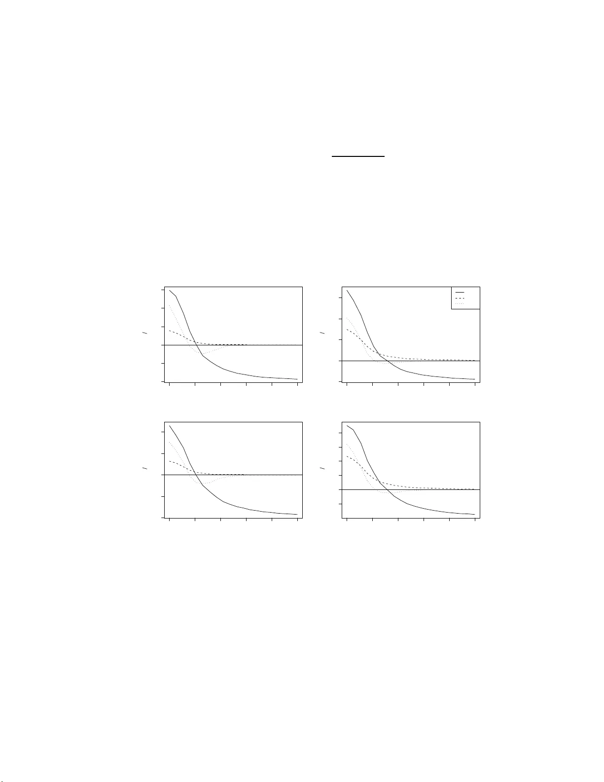
P ositiv e-shrink age and Pretest Estimation in Multiple Regression: A Mon te Carlo study with Applications SM Ena y etur Raheem 1 and S. Ejaz Ahmed University of Windsor, Windsor, ON, Canad a August 22, 2021 Abstract Consider a problem of p r edicting a resp ons e v ariable u sing a set of co v ariates in a linear regression mo del. If it is a priori kno wn or susp ected that a su bset of the co v ariates do not significan tly con tribute to the o verall fit of the mo del, a restricted mo del that excludes these co v ariates, ma y b e sufficient . If, on the other hand, the su b set pro vides usefu l information, shrink age metho d combines restricted and unrestricted estimators to obtain the p arameter estimates. Suc h an estimator outp erform s the classical maximum lik eliho o d estimators. Any prior information ma y b e v alidated through preliminary test (or p r etest), and dep end ing on the v alidity , ma y b e incorp orated in the mo del as a parametric restriction. Thus, pretest estimator c h o oses b et ween the restricted and unr estricted estimators dep endin g on the outcome of th e preliminary test. Examples using three r eal life data sets are p ro vided to illustr ate the ap p lication of shrink age and pretest estimation. P erformance of p ositive - shrink age and pretest estimators are compared with u nrestricted estimator un der v arying degree of un certain ty of the p r ior inf ormation. Monte Carlo study reconfirms the asymptotic prop erties of the estimators av ail able in the literature. Keywor ds and phr ases: J ames-Stein estimation; Shrink age estimation; Pretest estimation; Data analysis; Quadratic risk; Multiple r egression; RMSE; Mon te Carlo simulati on; lasso; 1 In tro duction Regression analysis is one of the most mature and widely applied br anc h in statistic s. Least squares estimation and r elated p ro cedures, mostly ha ving a parametric fla v or, hav e receiv ed considerable atten tion fr om theoretical as w ell as application p ersp ectiv es. Statistical mo d- els, b oth lin ear and n on-linear, are u sed to obtain in formation ab out u nkno wn parameters. Whether such mo del fits the data w ell or whether the estimated parameters are of m uc h use dep ends on the v alidit y of certain assumptions. In this setup, the estimates are obtained to h a ve insigh ts ab out the parameters. How ev er, in many p ractical situations, it is the re- searc h ers who pr o vid e the estimation of the parameters utilizing the information contai ned in the sample and other relev an t inform ation. The “other” in f ormation ma y b e considered as non-sample information (NSI). Th is is also kn own as unc ertain prior information (UPI), or simply prior information. The non-sample information may or ma y not p ositiv ely con- tribute in the estimation p r o cedure. Nev ertheless, it m a y b e adv an tageous to use the NSI in the estimation pr o cess wh en sample-information may b e rather limited. The qualit y of the fit an d of th e estimated parameters d ep end largely on the quality of the data used to obtain them. Only reliable information leads to useful resu lts. Ho we v er, in m any practical situations, uncertain t y arises as to w hether the a v ailable in formation is 1 Author for corresp ondence. Emai l: raheem@gmai l.com 1 of m uc h u se. It is widely accepted that in applied science, an exp erim ent is often p erformed with some prior kno wledge of the outcomes, or to confirm a hyp othetical result, or to re-establish existing r esu lts. With this k eeping in mind , it is ho w ev er, imp ortant to n ote that the consequences of incorp orating n on-sample information dep end on the qu alit y or u sefulness of the inform ation b eing add ed in th e estimation pro cess. An y uncertain prior inf ormation may b e tested b efore they are incorp orated in the mo del. Based on th e idea of Bancroft (1944), u ncertain prior in formation m ay b e v alidated th rough preliminary test, and d ep ending on the v alidit y , ma y b e in corp orated in as a parametric restriction, and choose b et ween the restricted or unrestricted estimation pr o cedure dep ending on th e outcome of the preliminary test. Later, Stein (1956) in tro duced shrink age estimatio n. In this fr amew ork , the shrink age estimator or Stein-t yp e estimator tak es a hybrid approac h by shrinkin g the b ase estimator to a plausible alternativ e estimator utilizing the non-samp le in formation if it pro v es to b e useful. 1.1 Review of Lit erature Since the b eginning, shrin k age estimation ha v e receiv ed considerable atten tion fr om the re- searc h ers. Sin ce 1987, Ah med and his co-researc hers are among others who ha v e analytically demonstrated that sh rink age estimators outshine th e classical maxim um lik eliho o d estima- tor. Asymptotic pr op erties of shrin k age and p r eliminary test estimators using quadr atic loss function ha ve b een studied, and their dominance o ver the usual maxim u m lik eliho o d estimators demonstrated in numerous studies in the literature. Ah m ed (1997) ga v e a d e- tailed description of shrin k age estimation, and discuss ed large samp le estimation tec hniques in a regression mo del with non-n ormal errors . Khan and Ahmed (2003 ) consider ed th e p r oblem of estimating the co efficien t ve ctor of a classical regression mo del, an d demonstrated analytically and numerically that the p ositiv e- part of Stein-t yp e estimator, and th e imp ro ved p reliminary test estimator d ominate the usual Stein-t yp e, and p r etest estimators, resp ectiv ely . Estimation of the mean v ector of a m ultiv ariate n ormal distrib ution, und er the un certain prior information that comp onent means are equal bu t unkn own, wa s studied by K han and Ahmed (2006). Ahmed and Nicol (2010) among others, considered v arious large sample estimation tec hniqu es in a nonlinear regression mo del. Nonparametric estimation of the lo cation parameter v ector w hen un certain prior inf ormation ab out the regression parameters is a v ailable wa s considered by Ahmed and S aleh (1999). In this pap er , w e review p ositiv e sh rink age, and pretest estimators to compare their p erformance when certain information ab out a subset of the co v ariates are a v ailable a priori . In particular, we apply shrink age estimation on three r eal life data sets to show the usabilit y of p ositiv e-shrink age and p retest estimators for practical pu rp oses. 2 Statemen t of the Problem Consider a regression mo del of the form Y = X β + ε , (2.1) where Y = ( y 1 , y 2 , . . . , y n ) ′ is a ve ctor of resp onses, X is an n × p fix ed design matrix, β = ( β 1 , . . . , β p ) ′ is an un kno wn parameter vecto r and ε = ( ε 1 , ε 2 , . . . , ε n ) ′ is the v ector of 2 unobserv able r andom errors, and the sup erscript ( ′ ) den otes the transp ose of a v ector or matrix. W e do not mak e any distribu tional assump tion for the err ors, only that ε s ha v e a cum ulativ e distrib u tion function F ( ε ) w ith E ( ε ) = b 0, and E ( εε ′ ) = σ 2 I , where σ 2 is finite. W e mak e the follo wing tw o assumptions, also called the regularit y cond itions i) max 1 ≤ i ≤ n x ′ i ( X ′ X ) − 1 x i − → 0 as n − → ∞ , wh er e x ′ i is th e i th ro w of X ii) lim n →∞  X ′ X n  = C n , where C n is a fin ite p ositive -definite matrix. In our case, sup p ose that β may b e partitioned as β = ( β ′ 1 , β ′ 2 ) ′ . The su b-v ectors β 1 and β 2 are assumed to ha v e dimensions p 1 and p 2 resp ectiv ely , and p 1 + p 2 = p , p i ≥ 0 for i = 1 , 2. Here, β 1 is the co efficien t vec tor for main effects, and β 2 is a ve ctor for “n uisance” effects. W e are essen tially inte rested in the estimatio n of β 1 when it is plausib le that β 2 do n ot contribute significantly in p redicting the r esp onse. Suc h a situation ma y arise when there is ov er-mo deling and one wishes to cut do wn the irrelev ant part from the mo del (2.1). F or example, in s tudying the relationship b et w een the level of prostate sp ecific anti gen (PSA) and s ome clinical measures, the log cancer volume and log pr ostate w eigh t can b e considered as the main effects while age, log of b enign prostate hyp erplasia amoun t, seminal vesicle in v asion and others can b e r egarded as n uisance v ariables. In this situation, inference ab out β 1 ma y b enefi t from shrinking the r egression co efficien ts of the full mo del tow ards the restricted space while u tilizing the av ailable in f ormation con tained in the n uisance co v ariates. T h us, the parameter space can b e partitioned, and it is plausib le that β 2 is near some sp ecified β o 2 , wh ic h , without loss of generalit y , ma y b e set to a null v ector. The pr ior in formation ab out the sub set of β can b e written in terms of a restriction, H β = h . Here, H is a kn o wn p 2 × p matrix and h is p 2 × 1 v ector of kn own constant s. 2.1 Organization of the Paper The pap er is organized as follo ws. The statistica l m o del is introdu ced in section 3. S hrink- age, p ositiv e-shrink age, and pretest estimators are d efined in this section. Examp les usin g three real life data sets are presen ted in section 4. Positiv e-shrink age and pr etest estima- tors are obtained, and their p erformance are compared using cross-v alidation. Mont e Carlo sim ulation s tudy is d escrib ed in section 5. Asymptotic b ias and risk expressions for the shrink age estimato rs are p resen ted in section 6. Finally , conclusions an d future d irections are presente d in section 7. 3 The Mo del and Estimation Strategies The least-squares estimator of β is giv en by ˆ β UR = ( X ′ X ) − 1 X ′ Y = C − 1 X ′ Y , where C = ( X ′ X ) . Un d er the r estriction H β = h , the restricted estimator is given by ˆ β R = ˆ β UR − C − 1 H ′ ( H C − 1 H ′ ) − 1 ( H ˆ β UR − h ) , 3 whic h is a linear fu nction of the unrestricted estimator. Let us define th e estimator of σ 2 b y s 2 e = ( Y − X ˆ β UR ) ′ ( Y − X ˆ β UR ) n − p . W e ma y consider testing th e restriction in the form of testing the null hyp othesis H 0 : H β = h . The test statistic is defin ed by ψ n = ( H ˆ β UR − h ) ′ ( H C − 1 H ′ ) − 1 ( H ˆ β UR − h ) s 2 e , (3.1) whic h, un der H 0 , follo w s a c hi-square d istribution with p 2 degrees of freedom. 3.1 Shrink age Estimator A Stein-t yp e estimator (STE) ˆ β S 1 of β 1 can b e defin ed as ˆ β S 1 = ˆ β R 1 + ( ˆ β UR 1 − ˆ β R 1 )  1 − κψ − 1 n  , where κ = p 2 − 2 , p 2 ≥ 3 . where ψ n is d efined in (3.1). One p roblem w ith STE is that its comp onen ts m ay ha v e a different sign from the co ordinates of ˆ β UR 1 . Th is could happ en if ( p 2 − 1) ψ − 1 n is larger than un it y . One p ossibilit y is when p 2 = 2 and ψ n < 1 . F r om the practical p oin t of view, the c hange of sign wo uld affect its interpretabilit y . How ev er, this b eha vior do es not adversely affect the risk p erformance of STE. T o o v ercome the sign p roblem, w e define a p ositive -rule Stein-type semiparametric estimator (PSTE) by retaining the p ositiv e-part of the STE. A PSTE has the form ˆ β S+ 1 = ˆ β R 1 + ( ˆ β UR 1 − ˆ β R 1 )  1 − κψ − 1 n  + , p 2 ≥ 3 where z + = max(0 , z ). Alternative ly , this can b e written as ˆ β S+ 1 = ˆ β R 1 + ( ˆ β UR 1 − ˆ β R 1 )  1 − κψ − 1 n  I ( ψ n < κ ) , p 2 ≥ 3 . Ahmed (2001) and others studied the asymptotic prop erties of Stein-type estimators in v arious con texts. 3.2 Preliminary T est Estimator The p reliminary test estimato r or pretest estimator for the regression p arameter β 1 is obtained as ˆ β PT 1 = ˆ β UR 1 − ( ˆ β UR 1 − ˆ β R 1 ) I ( ψ n < c n,α ) , (3.2) where I ( · ) is an indicator function, and c n,α is the upp er 100(1 − α ) p ercen tage p oint of th e test statistic ψ n . In a pretest estimation prob lem, the prior information is tested b efore c h o osing the esti- mator for practical p urp oses, wh ile shr ink age and p ositiv e-sh r ink age estimato r incorp orates in the estimation pr o cess wh atev er prior inf ormation is a v ailable. 4 Pretest estimator either accepts of rejects th e restricted estimator ( ˆ β R 1 ) based on whether ψ n < c n,α , w h ile shrink age estimator is a smo othed version of th e pr etest estimator. 4 Examples In th e follo wing, w e study th ree r eal life examples. F or eac h data s et, we fit linear r egression mo dels to pr edict the v ariable of in terest form the a v ailable regressors. Sh rink age and pretest estimates are then obtained for the r egression parameters. P erformance of shrink age and pretest estimators are assessed as p er th e criteria outlined in the follo w ing section. 4.1 Assessmen t Criteria In shrink age and pretest estimati on, w e utilize the full-mo del and su b-mo del estimates, and com bin e them in a wa y that shrinks th e least-squares estimates to wards the sub-mo del estimates. In this framewo rk, we utilize, if a v ailable, the information con tained in the restricted subsp ace if they contribute significan tly in predicting the resp onse. Ho wev er, in the absence of p rior information ab out the n uisance subset, one might d o usual v ariable selection to filter the nuisance su bset ou t of th e co v ariates. In that, one initiates the pro cess with th e mo del h a vin g all the co v ariates. Then th e b est subset may b e selected based on AIC, BIC or other mo del selection criteria. Separate estimates f rom fu ll- and restricted mo dels are then com bined to obtain sh rink age estimates. Finally , a m o del with shru nk en co efficien ts is obtained, whic h reduces o v erall prediction err or. W e obtain pr etest and p ositiv e-shrink age estimates u s ing different su b-mo dels. Perfor- mance of eac h p air of fu ll- and su b-mo dels w as ev aluated by estimating the pred iction error based on K -fold cross v alidation. In a cross v alidation, the d ata set is rand omly divided in to K su bsets of r oughly equal size. On e s ubset is left aside, and termed as test d ata, while the remaining K − 1 subsets, called training set, are used to fit the mo del. The fitted mo del is then used to p r edict the resp onses of the test data set. Finally , prediction errors are obtained b y taking the squared d eviation of the observ ed and predicted v alues in the test set. W e consider K = 5 , 10. Both ra w cross v alidation estimate (CVE), and bias corrected cross v alidation estimate of pr ediction errors are ob tained for eac h configuration. Th e bias corrected cross v alidation estimate is the adjus ted cross-v alidation estimate designed to comp ensate for the bias introdu ced by not u s ing lea v e-one-out cross-v alidation (Tibsh ir ani and Tibshir an i, 2009). Since cross v alidation is a random pro cess, the estimated p rediction error v aries across runs, an d f or differen t v alues of K . T o account for the r andom v ariation, we rep eat the cross v alidation pr o cess 5000 times, and estimate the av erage prediction errors along w ith their standard err ors. The num b er of rep etitio ns was in itially v aried, and settled with this as no noticeable v ariations in the standard errors w ere observed for higher v alues. 4.2 Prostate Data Hastie et al. (2009) demonstrated v arious mo d el selection tec hniques by fitting linear r e- gression mo del to the p rostate d ata. S p ecifically , the log of prostate-sp ecific an tigen ( lpsa ) w as mo deled by the log cancer v olume ( lcav ol ), log prostate weigh t ( lweight ), age ( age ), log b enign p rostatic hyp erplasia amoun t ( lb ph ), seminal v esicle in v asion ( svi ), log capsular 5 p enetration ( lcp ), Gleason score ( glea son ), and p ercenta ge Gleason scores 4 or 5 ( pgg45 ). The idea is to pr edict lpsa from the m easur ed v ariables. The p redictors were first stand ardized to ha v e zero mean and unit standard d eviation b efore fitting the mo del. Several mo d el selection criteria and shrink age metho ds w ere tried– details of whic h may b e found in Hastie et al. (2009 , T able 3.3, page 63). W e consider the mo dels obtained b y AIC, BIC, and b est subs et selection (BSS) criteria, and consider them as our sub-mo dels. They are listed in T able 1. T able 1: F u ll and candidate sub -mo dels f or p rostate data. Selection Criterion Mo del: Resp onse ˜ Cov ariates F u ll Mo del lpsa ˜ lc avol + l weight + svi + l bph + age + lcp + gleason + pgg45 AIC lpsa ˜ lcavol + lweig ht + svi + lbph + age BIC lpsa ˜ lcavol + lweig ht + svi BSS lps a ˜ lca vol + lw eight Av erage pr ediction errors, and their standard deviations for pretest an d shrink age esti- mators for v arious sub -mo dels are sho wn in T able 2. Prediction errors are based on five - and ten-fold cross v alidation. Av erage and standard errors are obtained after rep eating the pro cess 5000 times. T able 2: Averag e p rediction errors for v arious estimators based on K -fold cross v alidation rep eated 5000 times for prostate data. Nu m b ers in smaller fon t are the corresp onding standard errors. Ra w CVE Bias Corrected CVE Estimator K = 5 K = 10 K = 5 K = 10 UR .556 . 030 .548 . 018 .543 . 026 .542 . 017 R(AIC) .535 . 023 .529 . 014 .525 . 020 .523 . 013 R(BIC) .537 . 020 .533 . 012 .529 . 018 .529 . 011 R(BSS) .582 . 017 .578 . 010 .576 . 015 .576 . 009 PS(AIC) .554 . 029 .547 . 018 .540 . 025 .541 . 017 PS(BIC) .546 . 026 .541 . 016 .533 . 023 .535 . 015 PS(BSS) .549 . 026 .542 . 016 .536 . 023 .536 . 015 PT(AIC) .536 . 024 .529 . 014 .526 . 021 .525 . 014 PT(BIC) .538 . 021 .533 . 012 .529 . 019 .529 . 011 PT(BSS) .599 . 030 .601 . 024 .602 . 036 .605 . 029 Lo oking at the bias corrected cross v alidation estimate of the prediction errors, on an a verage , restricted and the pretest estimators based on AIC ha v e the smallest prediction errors. T his is follo w ed by pretest and the restricted estimators based on BIC. In terestingly , a verage prediction errors based on the sub-mo d el giv en by BSS is muc h h igher than those obtained from the mo d els based on AIC or BIC. F or instance, r estricted mo del based on 6 BSS has av erage prediction error 0.576 , and the same for pr etest estimator is 0.605. F or the same sub-mo del, p ositiv e-shrink age estimator has a v erage prediction error 0.536, w hic h is m uc h less than R(BSS ), and PT(BSS). Clearly , p ositiv e shrink age estimator is b eating the restricted and pretest estimators for this sub-mo d el. This is a classic example where utilit y of p ositive -shrink age estimator is practically realized. Restricte d and/or pretest estimation ma y p erform b etter u n der correct sp ecification of the mo d el (e.g., the mo d els giv en b y AIC and BIC for th is data set), whereas, p ositiv e-shr in k age estimator is less sensitive to mo d el missp ecification. Apparent ly , in the p resence of imprecise su bspace in f ormation, restricted and pr etest estimators f ail to pr o duce the b est estimates that r ed uce a v erage prediction errors. O n the other h an d , p ositiv e-shrink age estimator main tains a steady risk-sup eriorit y u nder mo del missp ecification. T h is b eha viour is illustrated in more detail through a Mon te Carlo study in section 5. 4.3 State Data F araw a y (2002) illustrated v ariable selection metho ds on a data set called state . T here are 97 observ ations (cases) on 9 v ariables. The v ariables are: p opulation estimate as of J u ly 1, 1975; p er capita income (1974); illiteracy (1970, p ercen t of p opu lation); life exp ectancy in yea rs (1969-71); m ur der and non-negligen t manslaugh ter rate p er 100,0 00 p opulation (1976 ); p ercen t h igh-sc h o ol grad u ates (1970); m ean n umber of days with minimum tem- p erature 32 d egrees (1931-1960 ) in capital or large cit y; and land area in square miles. W e consider life exp ectancy as the resp onse. It w as found that p opulation, m u rder, high sc ho ol graduates, and temp erature pr o duce the b est mo del based on AIC or BIC. A mo del based on CP statistic that includes p opulation, high sc ho ol graduates, and temp erature sho we d the largest adjusted R 2 . All the mo d els are listed in T able 3. T able 3: F u ll and candidate sub -mo dels for s tate data. Selection Criterion Mo del: Resp onse ˜ Co v ariates F u ll Life.exp ˜ Popu lation + Murder + Hs. grad + Frost + Income + Il literacy + A rea AIC/BIC Life.exp ˜ P opulation + Murder + Hs .grad + Frost CP Life.exp ˜ M urder + Hs.grad + F rost When the mod els are correctly sp ecified, it is ob vious that restricted estimator will p erform the b est. Su c h is the scenario for the state d ata, where the mod el giv en by AIC and BIC are the same, and the restricted estimator h as the smallest prediction error. Under mo del uncertain t y , ho wev er, the scenario will c hange completely as restricted estimator b ecomes u n b ound ed when the sub-mo d el deviates f rom th e true structure. T his is explored in the simula tion study p resen ted in section 5. F or the correctly sp ecified mo dels, su c h as in T able 4, we see that restricted and pr etest estimators ha v e the s m allest a verage prediction errors f or b oth fi v e-fold and ten-fold cr oss v alidation. The bias corrected v ersion of the cross v alidation errors are exactly th e same for the restricted and pr etest estimators. 4.4 Galapagos Dat a 7 T able 4: Ave rage prediction errors (thousands) f or v arious estimators b ased on K -fold cross v alidation, rep eated 5000 times for state data. Num b ers in smaller font are th e corresp onding standard errors. Ra w CVE Bias Corrected CVE Estimator K = 5 K = 10 K = 5 K = 10 UR .879 . 144 .847 . 086 .819 . 119 .820 . 079 R(AIC) .637 . 063 .614 . 036 .599 . 052 .597 . 033 R(CP) .639 . 058 .639 . 033 .626 . 048 .626 . 031 PS(AIC) .740 . 124 .690 . 074 .696 . 104 .671 . 068 PS(CP) .768 . 106 .746 . 063 .727 . 090 .727 . 058 PT(AIC) .637 . 066 .614 . 036 .599 . 054 .597 . 033 PT(CP) .662 . 069 .639 . 035 .629 . 059 .626 . 032 F araw a y (2002) analyzed th e data ab out sp ecies diversit y on th e Galapagos islands. Th e Galapago s data cont ains 30 ro ws and seven v ariables. Eac h r o w represen ts an island, and the co v ariates represent v arious geographic measuremen ts. Th e relationship b et ween the n umber of sp ecies of tortoise and sev eral geographic v ariables is of interest. The data set has the follo wing co v ariates: Sp ecies r epresen ts the n umber of sp ecies of tortoise foun d on the island, Endemics represent s the n um b er of endemic sp ecies, Area represents the area of the island (km 2 ), E levation measur es the h ighest elev ation of the island (m), Nearest is the distance from th e nearest island (km), S cruz measur es the distance from Sant a Cruz island (km), Adja cent measur es the area of the adjacen t island (km 2 ). The original d ata set con tained missing v alues for some of th e co v ariates, whic h ha v e b een imp uted by F araw a y (2002 ) for con v enience. The full mo del and the su b-mo dels based on AIC and BIC are sho wn in T able 5. T able 5: F u ll and candidate sub -mo dels f or Galapagos data. Selection Criterion Mo del: Resp ons e ˜ Co v ariates F u ll Species ˜ Endemic s + Are a + Elevation + N earest + Scruz + Adjacen t AIC Species ˜ End emics + Area + E levation BIC Species ˜ End emics W e obtain restricted, p retest, and p ositiv e-shrin k age estimates of the regression p aram- eters of the Galapagos data. Av erage prediction errors along with their stand ard errors f or unrestricted (UR), restricted (R), p ositiv e-shrink age (PS ), and pr eliminary test or pretest (PT) estimators are pr esented in T ab le 6. Prediction errors and the standard er r ors are sho wn in thousan d s. PS (AIC) represents p ositiv e shrink age estimates based on sub -mo del giv en by AIC, and PS(BIC) represents the same based on BIC. PT(AIC) and PT(BIC) are similarly defined for pretest estimators. F or this example as we ll, since we ha v e selected our su b-mo dels based on AIC or BIC, 8 T able 6: Ave rage prediction errors (thousands) f or v arious estimators b ased on K -fold cross v alidation, rep eated 5000 times for Galapagos data. Nu m b ers in s maller fon t are th e corresp onding standard errors. Ra w CVE Bias Corrected CVE Estimator K = 5 K = 10 K = 5 K = 10 UR 13.87 8 . 36 12.63 4 . 36 11.31 6 . 70 11.48 3 . 93 R(AIC) 12.45 6 . 96 11.62 4 . 28 10.10 5 . 57 10.53 3 . 85 R(BIC) 1.78 0 . 59 1.65 0 . 24 1.46 0 . 43 1.51 0 . 29 PS(AIC) 13.19 7 . 82 11.98 4 . 29 10.75 6 . 27 10.88 3 . 87 PS(BIC) 9.07 6 . 53 7.96 3 . 75 7.54 5 . 24 7.32 3 . 38 PT(AIC) 12.50 6 . 98 11.63 4 . 29 10.14 5 . 58 10.54 3 . 86 PT(BIC) 5.39 7 . 56 3.90 6 . 16 4.40 6 . 08 3.55 5 . 56 they are lik ely to b e true, which r esults in r estricted and pr etest estimators b eing the b est estimators in terms of prediction errors. W e notice th at, mo d els b ased on BIC are smaller in size, and th eir a v erage prediction err ors are smaller than those of the AIC m o dels. The difference in av erage p rediction errors for the t wo sub-mo d els is n oticea bly large. Suc h a large difference b etw een the comp eting sub -mo dels sho ws u s ab out the uncertaint y in mo d el sp ecification, and the consequences that it cause. Mon te Carlo study conducted later in the pap er (section 5) rev eals the sensitivit y of restricted and pretest estimators, and sho w s that pretest and restricted estimators are outp erformed by p ositive -shrink age estimators when the und erlying mo del is missp ecified. It is n oted here that the prediction errors are unusually large for this data set. This indicates that the pr ed ictors are not qu ite capturing the v ariabilit y in the resp onse. 5 Sim ulation Studies Mon te Carlo simulatio n exp eriment s hav e b een conducted to examine the quadr atic risk p erformance of p ositiv e-shr in k age and pretest estimators. W e simulat e the resp onse from the follo w ing mo d el: y i = x 1 i β 1 + x 2 i β 2 + . . . , + x pi β p + ε i , i = 1 , . . . , n, where x 1 i = ( ζ (1) 1 i ) 2 + ζ (1) i + ξ 1 i , x 2 i = ( ζ (1) 2 i ) 2 + ζ (1) i + 2 ξ 2 i , x si = ( ζ (1) si ) 2 + ζ (1) i with ζ (1) si i.i.d. ∼ N (0 , 1), ζ (1) i i.i.d. ∼ N (0 , 1), ξ 1 i ∼ Bernoulli(0.45) an d ξ 2 i ∼ Bernoulli(0.45) for all s = 3 , . . . , p and i = 1 , . . . , n . Moreo ver, ε i are i.i.d. N (0 , 1). W e are intereste d in testing the hypothesis H 0 : β j = 0 , f or j = p 1 + 1 , p 1 + 2 , . . . , p 1 + p 2 , with p = p 1 + p 2 . Accordingly , we partition the r egression co efficien ts as β = ( β 1 , β 2 ) = ( β 1 , 0 ). W e sho w results f or β 1 = (1 , 1 , 1), and β 1 = (1 , 1 , 1 , 1) only . The num b er of simulatio ns were initially v aried. Finally , eac h realization wa s rep eated 2000 times to obtain stable results. F or eac h realizati on, we calculate d bias of the estimators. W e defined ∆ = || β − β (0) || , where β (0) = ( β 1 , 0 ), and || · || is the Euclidean n orm. T o 9 determine the b eha vior of the estimators for ∆ > 0 , fu r ther data sets were generated fr om those d istr ibutions under lo cal alternativ e hyp othesis. V arious ∆ v alues b et wee n [0,1] ha v e b een considered. The risk p erformance of an estimator of β 1 w as measured by comparing its MS E with that of the unrestricted estimator as defined b elo w: RMSE( ˆ β UR 1 : ˆ β * 1 ) = MSE( ˆ β UR 1 ) MSE( ˆ β * 1 ) , (5.1) where ˆ β * 1 is one of th e estimators considered in this study . Th e amoun t b y wh ic h an RMSE is larger than un ity indicates the degree of sup eriority of th e estimator ˆ β * 1 o ver ˆ β UR 1 . RMSEs for the p ositiv e-shrink age and p retest estimat ors w ere computed for n = 30 , 50 , 100 , p 1 = 3 , 6 , 9, and p 2 = 4 , 6 , 9. Since the results are sim ilar for all the configurations, we list the RMSE s in T able 7 f or n = 50. Comparativ e RMSEs for p ositiv e-shrink age and p retest estimators for ( p 1 , p 2 ) = (3, 3), (3, 6), (4, 3), and (4, 6) are illus tr ated in Figure 1. 0.0 0.2 0.4 0.6 0.8 1.0 0.0 0.5 1.0 1.5 2.0 2.5 ( a ) p 1 = 3, p 2 = 3 ∆ β ^ UR β ^ * 0.0 0.2 0.4 0.6 0.8 1.0 0 1 2 3 4 ( b ) p 1 = 3, p 2 = 6 ∆ β ^ UR β ^ * RES S+ PT 0.0 0.2 0.4 0.6 0.8 1.0 0.0 0.5 1.0 1.5 2.0 ( c ) p 1 = 4, p 2 = 3 ∆ β ^ UR β ^ * 0.0 0.2 0.4 0.6 0.8 1.0 0.5 1.0 1.5 2.0 2.5 3.0 ( d ) p 1 = 4, p 2 = 6 ∆ β ^ UR β ^ * Figure 1: Relativ e mean squared error for restricted, p ositiv e-shrink age, and pr etest esti- mators for n = 50, and ( p 1 , p 2 ) = (3, 3), (3, 6), (4, 3), and (4, 5) 5.1 Case 1: ∆ = 0 Clearly , f or ∆ = 0, the restricted estimator ou tp erforms all other estimators for all the cases considered in th e simulatio n stud y . As the restriction mo v es a w a y fr om ∆ = 0 , the restricted estimator b ecomes u n b ound ed (see th e sharp ly deca yin g curve that go es b elo w the horizon tal line at ˆ β UR 1 / ˆ β * 1 =1 for ∆ > 0). T he p ositive -shrink age estimator appr oac hes 1 at the slo west rate (for a range of ∆) as w e mo ve a wa y from ∆ = 0. This indicates that in the ev ent of impr ecise subspace inf orm ation (i.e., ev en if β 2 6 = 0 ), it h as the smallest quadr atic 10 T able 7: Simulate d r elativ e mean squ ared err or for restricted, p ositiv e-shrink age, and pretest estimators with resp ect to un restricted estimator for p 1 = 4 , and p 2 = 6 for differen t ∆ when n = 50. ∆ ∗ ˆ β R 1 ˆ β S+ 1 ˆ β PT 0.00 3.25 2.17 2.59 0.05 3.10 2.06 2.30 0.11 2.63 1.83 1.77 0.16 2.02 1.57 1.31 0.21 1.60 1.39 1.04 0.26 1.23 1.27 0.91 0.32 0.98 1.20 0.89 0.37 0.77 1.15 0.89 0.42 0.63 1.12 0.93 0.47 0.51 1.09 0.96 0.53 0.42 1.07 0.98 0.58 0.36 1.06 0.99 0.63 0.31 1.06 1.00 0.68 0.27 1.05 1.00 0.74 0.23 1.04 1.00 0.79 0.20 1.03 1.00 0.84 0.18 1.03 1.00 0.89 0.16 1.02 1.00 0.95 0.15 1.03 1.00 1.00 0.13 1.02 1.00 risk among all other estimators for a range of ∆. Pretest estimator outshines shr ink age estimators w hen ∆ is in the n eigh b ourho o d of zero. Otherwise, it b ecomes unb ounded at a f aster rate than the restricted estimator. Ho wev er, w ith the increase of ∆, at some p oint , RMSE of pretest estimator approac hes 1 from b elo w. This phenomenon s uggests that neither pr etest nor restricted estimator is u niformly b etter than the other w h en ∆ > 0. 5.2 Case 2: ∆ > 0 Sim ulation resu lts suggest that p ositiv e shrink age estimator mainta ins its sup eriorit y o ve r the restricted and pretest estimators f or a wid e range of ∆ . I n particular, when p 2 = 3, the p erform an ce of p ositiv e-shr ink age estimator is sup erior for ∆ u p to aroun d 0.35, after whic h p oint it is as go o d as the unrestricted estimator (panels a) and c) in Figure 1). Ho wev er, wh en p 2 = 6, p ositiv e-shrink age estimator m ain tains its risk-sup eriorit y o ver all other estimators for a wider r ange of ∆ (see p anels b) an d d ) in Figure 1). Th is clearly suggests that a p ositiv e-shrink age estimator is preferr ed as there alw a ys remains uncertain t y in sp ecifying statistical mo d els correctly . Moreo v er, on e cannot go wrong with the p ositiv e- shrink age estimators ev en if the assumed mo del is grossly wrong. In suc h cases, the estimates are as go o d or equal to the un restricted (i.e., full mo del) estimates. In the follo wing s ections, w e review the asymptotic prop erties of the estimators, and analyticall y pr esen t their bias and risk expressions. 11 6 Asymptotic Distribution of the Estimators In this section we pr esen t the asymptotic distr ib utions of th e estimators, and the test statistic ψ n . This f acilita tes in find ing the asymptotic distr ibutional bias (ADB), asymp totic quadratic distribu tional bias (AQDB ), and quadratic risk (A QDR) of the estimator of β . Under fixed alternativ e, the asymp totic distrib u tion of √ n ( β ∗ − β ) /s e is equiv alen t to √ n ( ˆ β UR − β ) /s e . T his suggest th at in asymptotic setup, there is not muc h to inv estigate under a fi xed alternativ e suc h as H β 6 = h . Therefore, to obtain meaningful asymp totics, a class of lo cal alternativ es, { K n } , is considered, which is giv en by K n : H β = h + ω √ n , (6.1) where ω = ( ω 1 , ω 2 , · · · , ω p 2 ) ′ ∈ R p 2 is a fixed vec tor. W e notice that ω = 0 imp lies H β = h , i.e., the fi xed alternativ e is a p articular case of (6.1). In the f ollo wing, we ev aluate the p erformance of eac h estimators under lo cal alternativ e. F or an estimator β ∗ and a p ositiv e-definite matrix W , w e defin e th e loss f unction of the form L ( β ∗ ; β ) = n ( β ∗ − β ) ′ W ( β ∗ − β ) . These loss fu nctions are generally kno wn as weig ht ed quad r atic loss functions, wh ere W is the we igh ting matrix. F or W = I , it is the simple squared error loss fu nction. The exp ectation of the loss fu nction E [ L ( β ∗ , β ); W ] = R [( β ∗ , β ); W ] , is called the risk fu nction, wh ic h can b e written as R ( β ∗ , β ); W ) = n E [( β ∗ − β ) ′ W ( β ∗ − β )] = n tr[ W { E ( β ∗ − β )( β ∗ − β ) ′ } ] = tr( W Γ ∗ ) , (6.2) where Γ ∗ is th e co v ariance matrix of β ∗ . The p erformance of the estimators can b e ev aluated b y comparing the r isk functions with a suitable matrix W . An estimator with a smaller risk is p referred. The estimator β ∗ will b e called inadmissible if th ere exists another estimator β 0 suc h that R ( β 0 , β ) ≤ R ( β ∗ , β ) ∀ ( β , W ) (6.3) with strict in equalit y holds for some β . In su c h case, w e say that the estimator β 0 dominates β ∗ . If, ho w ev er, in s tead of (6.3) h olding for eve ry n , w e ha v e lim n →∞ R ( β 0 , β ) ≤ lim n →∞ R ( β ∗ , β ) ∀ β , (6.4) with strict in equalit y for some β , then β ∗ is termed as asymptotically inadmissible estimator of β . The expr ession in (6.3) is not easy to p ro v e. A n alternativ e is to consid er the asymptotic distrib utional quadratic risk (ADQR) f or the sequence of local alternativ e { K n } . Consider th e asymptotic cum ulativ e distrib u tion function (cdf ) of √ n ( β ∗ − β ) /s e under 12 { K n } exists, and defin ed as G ( y ) = lim n →∞ P [ √ n ( β ∗ − β ) /s e ≤ y ] . This is kno wn as the asymptotic d istribution function (ADF) of β ∗ . F ur ther let Γ = Z Z · · · Z y y ′ G ( y ) b e the disp ersion matrix whic h is obtained from ADF, the ADQR ma y b e defin ed as R ( β ∗ ; β ) = tr( W Γ ) . (6.5) An estimator β ∗ is said to dominate an estimator β 0 asymptotically if R ( β ∗ ; β ) ≤ R ( β 0 ; β ). F urther, β ∗ strictly dominates β 0 if R ( β ∗ ; β ) < R ( β 0 ; β ) for some ( β , W ). The asymptotic risk may b e ob tained b y replacing Γ with the limit of the actual d isp ersion matrix of √ n ( β ∗ − β ) in the ADQR fu nction. Ho wev er, this may require some extra regularit y conditions. Sen (1986), and Saleh and Sen (1985) among others, ha v e explained this p oint in v arious other conte xts. 6.1 Asymptotic Bias and R isk Performance T o ob tain the asymptotic distr ib ution of the prop osed estimators, and the test s tatistic ψ n , w e consider the follo wing th eorem. Theorem 6.1. Under the r e gu larity c onditions, and if σ 2 < ∞ , as n → ∞ , √ n s − 1 e ( ˆ β UR − β ) d ∼ N p ( 0 , C − 1 ) . 6.1.1 Bias Performance The asymptotic distrib utional bias (ADB) of an estimator δ is d efined as ADB( δ ) = lim n →∞ E n n 1 2 ( δ − β 1 ) o . Theorem 6.2. Under th e assume d r e gu larity c onditions and the or em ab ove, and under { K n } , the ADB of the estimators ar e as fol lows: ADB ( ˆ β UR 1 ) = 0 (6.6) ADB ( ˆ β R 1 ) = − C − 1 n H B − 1 ω (6.7) ADB ( ˆ β PT 1 ) = − C − 1 H B − 1 δ H p 2 +2 ( χ 2 p 2 ,α ; ∆) (6.8) ADB ( ˆ β S+ 1 ) = − C − 1 H B − 1 ω h H p 2 +2 ( p 2 − 2; ∆) + ( p 2 − 2) E n χ − 2 p 2 +2 (∆) o + E n χ − 2 p 2 +2 (∆) I ( χ 2 p 2 +2 (∆) > p 2 − 2) oi (6.9) where E ( χ − 2 j p (∆)) = Z ∞ 0 x − 2 j d Φ p ( x ; ∆) 13 and Φ p ( x ; ∆) is the cdf of a p -v ariate normal d istribution with mean v ector 0 , and co v ariance matrix, ∆. The bias expressions for all the estimators are n ot in th e scalar form . W e therefore tak e recourse by conv erting them in to the qu ad r atic form. L et u s define the asymptotic quadratic distribu tional bias (AQDB ) of an estimator δ of β 1 b y AQD B ( δ ) = [ AD B ( δ )] ′ Σ [ AD B ( δ )] where Σ − 1 = σ 2 C − 1 is th e disp ersion matrix of ˆ β UR as n → ∞ . Using the definition, and follo wing Ah med (1997 ), the asymptotic quadr atic distribu- tional bias of the v arious estimators are p resen ted b elo w. A Q DB( ˆ β UR 1 ) = 0 , (6.10) A Q DB( ˆ β R 1 ) = ξ ′ ξ σ 2 C − 1 = ∆ (6.11) A Q DB( ˆ β PT 1 ) = ∆  H p 2 +2 ( χ 2 p 2 ,α ; ∆)  2 (6.12) AD QB ( ˆ β S+ 1 ) = ∆ h H p 2 +2 ( p 2 − 2; ∆) + ( p 2 − 2) E n χ − 2 p 2 +2 (∆) o + E n χ − 2 p 2 +2 (∆) I ( χ 2 p 2 +2 (∆) > p 2 − 2) oi . (6.13) 6.1.2 Risk Performanc e F ollo wing Ahmed (1997), we pr esen t the r isk exp ressions of th e estimators. Theorem 6.3. Under the assume d r e gularity c onditions, and lo c al alternative { K n } , the ADQR expr essions ar e as fol lows: R ( ˆ β UR 1 ; W ) = σ 2 tr( W C − 1 ) (6.14) R ( ˆ β R 1 ; W ) = σ 2 tr( W C − 1 ) − σ 2 tr( Q ) + ω ′ B − 1 Qω (6.15) R ( ˆ β S 1 ; W ) = σ 2 tr( W C − 1 ) − ( p 2 − 2) σ 2 tr( Q 11 ) n 2 E [ χ − 4 p 2 +4 (∆)] − ( p 2 − 2) E [ χ − 4 p 2 +4 (∆)] o + ( p 2 − 2)( p 2 + 6)( γ ′ 1 Q 11 γ 1 ) E [ χ − 4 p 2 +4 (∆)] (6.16) R ( ˆ β PT 1 ; W ) = σ 2 tr( W C − 1 ) − σ 2 tr( Q ) H p 2 +2 ( χ 2 p 2 ,α ; ∆) + ω ′ B − 1 ω  2 H p 2 +2 ( χ 2 p 2 ,α ; ∆) − H p 2 +4 ( χ 2 p 2 ,α ; ∆)  (6.17) R ( ˆ β S+ 1 ; W ) = R ( ˆ β S 1 ; W ) + ( p 2 − 2) σ 2 tr( Q ) h E n χ − 2 p 2 +2 (∆) I ( χ 2 p 2 +2 (∆) ≤ p 2 − 2) o − ( p 2 − 2) E n χ − 4 p +2+2 (∆) I ( χ 2 p 2 +2 (∆) ≤ p 2 − 2) oi − σ 2 tr( Q ) H p 2 +2 ( p 2 − 2; ∆) + ω ′ B − 1 Qω { 2 H p 2 +4 ( p 2 − 2; ∆) } − ( p 2 − 2) ω ′ B − 1 Qω h 2 E n χ − 2 p 2 +2 (∆) I ( χ 2 p 2 +2 (∆) ≤ p 2 − 2) o − 2 E n χ − 2 p 2 +4 (∆) I ( χ 2 p 2 +4 (∆) ≤ p 2 − 2) o + ( p 2 − 2) E n χ − 4 p 2 +4 (∆) I ( χ − 4 p 2 +4 (∆) ≤ p 2 − 2) oi , (6.18) 14 where Q = H C − 1 W C − 1 H ′ B − 1 . Ahmed (1997) ha v e stud ied the statistical prop er ties of v arious shrink age and pretest estimators. It w as remark ed that none of the unrestricted, r estricted, and pretest estimators is inadmissible with resp ect to an y of th e others. Ho w ev er, at ∆ = 0, ˆ β R 1 ≻ ˆ β P 1 ≻ ˆ β UR 1 . Therefore, for all (∆; W ) and p 2 ≥ 3, R ( ˆ β S+ 1 ; W ) ≤ R ( ˆ β S 1 ; W ) ≤ R ( ˆ β UR 1 ; W ) is satisfied. T h us, we conclude that ˆ β S+ 1 p erforms b etter than ˆ β UR 1 in the ent ire parameter space induced by ∆. The gain in risk ov er ˆ β UR 1 is subs tan tial wh en ∆ = 0 or near. 7 Discussion In this pap er, we reviewe d p ositiv e-shrink age and pretest estimation in the con text of a m ultiple linear regression mo d el. In our stud y , w e pr esen ted asymptotic bias and the risk expressions for the estimators. When we ha v e pr ior inf orm ation ab out certain cov ariates, shrink age estimators are di- rectly obtained b y com bining the full and sub -mo del estimates. On the other hand, if a priori information is not a v ailable, sh rink age estimation tak es a tw o-step approac h in ob- taining the estimates. In the firs t step, a set of co v ariates are s elected based on a suitable mo del selectio n criterion such as AIC , BIC or b est sub set selection. Consequen tly , th e re- maining co v ariates b ecome nuisance, whic h form s a p arametric restriction on the fu ll mo del. In the second step, full and s ub-mo del estimates are com bined in a wa y th at minimizes the quadratic risk. T o illustr ate the m etho ds, th ree different d ata sets ha v e b een consid ered to obtain r e- stricted, p ositive shrink age, and pretest estimators. Ave rage prediction errors b ased on rep eated cross v alidation estimate of the error rates sh o ws that pretest and r estricted esti- mators h a ve sup erior risk p erformance compared to the unr estricted, and p ositiv e-shrink age estimators when the u nderlying mo d el is correctly sp ecified. This is not unusual sin ce th e restricted estimator dominates all other estimators when the prior information is correct. Since the data consid ered in th is study hav e b een interacti v ely analyzed using v arious mo del selection criteria, it is exp ected that the sub -mo dels consist of the b est subs ets of the a v ail- able co v ariates for the r esp ectiv e data s ets. T h eoreticall y , this is equiv alen t to the case where ∆ = 0, or ve ry close to zero. Th e real data examp les, how ev er, d o not tell us ho w sensitiv e are the prediction errors un d er mo del missp ecification. Therefore, we conduct Mon te Carlo sim ulation to study su c h c haracteristics for p ositiv e-shrink age and pretest estimators under v arying ∆, and different sizes of the nuisance sub sets. In Mont e Carlo study , we n u merically compu ted relativ e mean s quared errors for the restricted, p ositiv e-shrink age, and pr etest estimators w ith resp ect to the unr estricted es- timator. Our study r e-established th e f act that the restricted estimator outp erforms the unrestricted estimator at or near the p iv ot (∆ = 0). How ev er, as we deviate f r om the piv ot (∆ > 0), risk of the r estricted estimator b ecomes unb ounded. Pretest estimator b e- comes u n b oun d ed ev en faster than the r estricted estimator for the cases considered in the sim ulation. Ho wev er, as the ∆ incr eases, pretest estimator p erform s b etter for some ∆, and appr oac hes from b elo w to merge with the lin e where RMS E is u nit y . On the other 15 hand, p ositiv e-shrin k age estimator d eca ys at the slo w est rate with the increase of ∆, and p erform s teadily th roughout a wider r an ge of th e alternativ e parameter sub space. In partic- ular, when the nuisance subset is large, p ositiv e-shrink age estimators outp erforms all other estimators, which can b e seen in panels b) and d) in Figure 1. 7.1 F uture directions Pretest estimator either selects r estricted or u nrestricted estimator dep end ing on the sig- nificance b ased on a test statistic, while p ositiv e-shrink age estimator shrinks the co v ariates to wards the restricted sub s pace. The n uisance sub s et is ideally a null space when they do not con trib ute an yth ing to w ards the estimation pro cess. In this sense, shrink age estimators resem ble p en alized estimators su c h as the least abs olute p enalt y and selection operator, lasso . Prop osed by Tib shirani (1996), lasso is a member of the p enalized least squares (PLS) family , wh ic h p erforms v ariable selection and p arameter estimation sim ultaneously . Lasso estimates are obtained via cyclical co ordin ate d escen t algorithm. Shrink age estimation do es v ariable selection by shrinking the co efficien ts tow ards the restricted sub -space. In doing so, some of th e co efficien ts shrink tow ards zero, while some o ver-shrinks–pro du cing a n egativ e sign for th e co efficien t. Th e c hange of sign ma y b e uncomfortable for pr actitio ners, although it d o es not affect the risk p erformance. The p ositiv e-part shrink age estimator tak es care of the negativ e part by setting the co efficien t to exactly zero. In the pro cess, most of the co efficien ts are sh runk while some of them are eliminated by shrin king to zero. Since the int ro du ction of lasso, there has b een a tremendous amount of develo pment in lasso an d related absolute p enalt y estimation (APE) d uring the past one and a h alf decade. Although the lasso and shrink age metho ds h a ve b een around for quite some time, little w ork h as b een done to compare th eir relativ e p erform ance. Recen tly , Ahm ed et al. (2007) compared p ositiv e shrink age and lasso in a p artially linear regression setup. Ho wev er, no comparativ e study for shrink age and absolute p enalt y estimators in multiple linear regres- sion mo del has b een found in the review ed literature. W e are current ly wo rking on th is fron t, and the find ings will b e dissemin ated through fu ture communicati ons. References Ahmed, S. E. (1997). Asymptotic shr ink age estimation: the regression case. A pplie d Sta- tistic al Scienc e II , pages 113–13 9. Ahmed, S . E. (2001). S hrink age estimation of regression coefficients from censored data with multiple obser v ations. In Ahm ed , S . and Reid, N., editors, Empiric al Bayes and Likeliho o d Infer enc e, L e ctur e N otes in Statistics , v olume 148, pages 103–12 0. Springer- V erlag, New Y ork. Ahmed, S . E., Doksum, K. A., Hossain, S., and Y ou, J. (2007). Sh rink age, pretest and absolute p enalt y estimators in partially linear mo d els. Austr alian & N ew Ze aland Journal of Statistics , 49:435–4 54. Ahmed, S. E. and Nicol, C. J. (2010). An app licatio n of shrink age estimation to the nonlinear regression mo del. Computational Statistics & Data Analysis , In Press. Ahmed, S. E. and Saleh, A. E. (1999 ). Impro ved nonparametric estimation of lo cation v ectors in multiv ariate regression mo d els. J ournal of Nonp ar ametric Statistics , 11. 16 Bancroft, T. A. (1944). On biases in estimation due to the use of preliminary tests of significances. Annals of Mathematic al Statistics , 15:190 –204. F araw a y , J. J. (2002). Pr actic al R e gr ession and Anova using R . Hastie, T., Tibshir ani, R., and F riedman, J. (2009). The Elements of Statistic al L e arning: Data M ining, Infer enc e and Pr e diction . Spr inger. Khan, B. and Ahmed, S. (2006). Comparisons of impro v ed risk estimators of the multiv ariate mean v ector. Computational Statistics & D ata Anal ysis , 50(2):402 – 421. Khan, B. U. and Ahmed, S . E. (2003). Improv ed estimation of coefficient ve ctor in a regres- sion m o del. Communic ations in Statistics - Simulation and Computation , 32(3):747 –769. Saleh, A. K. M. E. and Sen, P . K. (1985). O n shr ink age m-estimator of lo cation p arameters. Communic ations in Statistics–The ory & M etho ds , 14:231 3–2329 . Sen, P . K. (1986). On the asymptotic distributional risk shrin k age and preliminary test v aersion of the mean of a multiv ariate n orm al distrib ution. Sankhya , 48:354–371 . Stein, C. (1956). The admissibilit y of hotelling’s t 2 -test. Mathematic al Statistics , 27:616– 623. Tibshirani, R. (1996). Regression sh r ink age and selection via th e lasso. Journal of the R oyal Statistic al So ciety: Series B , p ages 267–288. Tibshirani, R. J. and Tibs h irani, R. (200 9). A bias correction f or the m inim um err or rate in cross-v alidation. Annals of Applie d Statistics , 3(2):82 2–829. 17