Robust Kernel Density Estimation

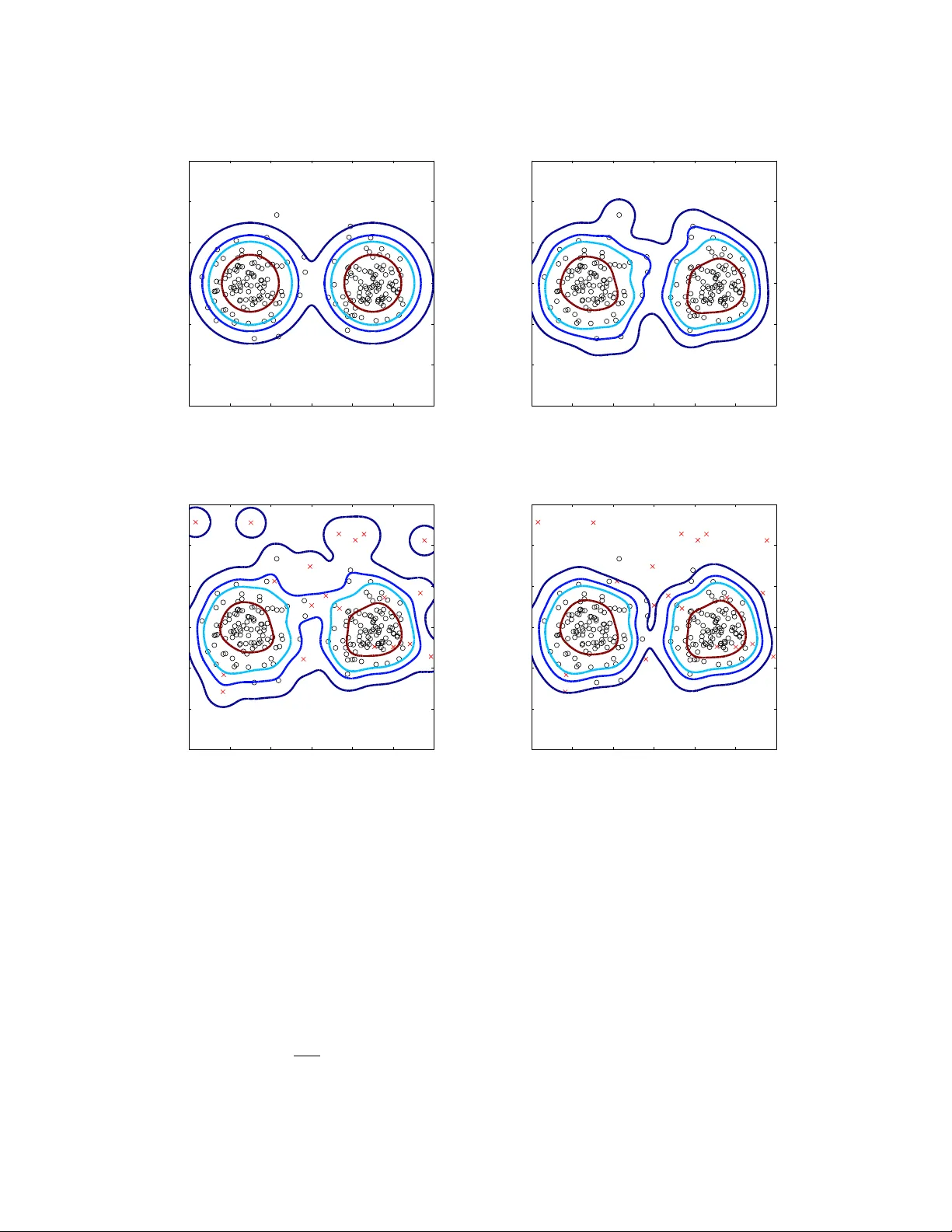
Robust Kernel Densit y Estimation Jo oSeuk Kim 1 and Cla yton D. Scott 1 , 2 1 Electrical Engineering and Computer Science, 2 Statistics Univ ersity of Mic higan, Ann Arb or, MI 48109-2122 USA email: { stannum, clayscot } @umich.edu No vem ber 27, 2024 Abstract W e prop ose a method for nonparametric density estimation that exhibits robustness to con tamination of the training sample. This method ac hieves robustness b y com bining a traditional kernel densit y estimator (KDE) with ideas from classical M -estimation. W e interpret the KDE based on a radial, p ositive semi-definite kernel as a sample mean in the asso ciated reproducing kernel Hilb ert space. Since the sample mean is sensitive to outliers, we estimate it robustly via M -estimation, yielding a robust k ernel densit y estimator (RKDE). An RKDE can b e computed efficien tly via a kernelized iteratively re-weigh ted least squares (IR WLS) algorithm. Necessary and sufficient conditions are giv en for k ernelized IR WLS to con verge to the global minimizer of the M -estimator ob jectiv e function. The robustness of the RKDE is demonstrated with a represen ter theorem, the influence function, and exp erimen tal results for density estimation and anomaly detection. Keywords : outlier, repro ducing kernel feature space, k ernel tric k, influence function, M - estimation 1 In tro duction The kernel density estimator (KDE) is a well-kno wn nonparametric estimator of univ ariate or multiv ariate densities, and n umerous articles ha ve b een written on its prop erties, appli- cations, and extensions (Silv erman, 1986; Scott, 1992). How ev er, relatively little work has b een done to understand or impro ve the KDE in situations where the training sample is con taminated. This pap er addresses a metho d of nonparametric density estimation that 1 generalizes the KDE, and exhibits robustness to con tamination of the training sample. Consider training data following a contamination model X 1 , . . . , X n iid ∼ (1 − p ) f 0 + pf 1 , (1) where f 0 is the “nominal” density to b e estimated, f 1 is the density of the contaminating distribution, and p < 1 2 is the proportion of contamination. Lab els are not a v ailable, so that the problem is unsup ervised. The ob jectiv e is to estimate f 0 while making no parametric assumptions ab out the nominal or con taminating distributions. Clearly f 0 cannot b e recov ered if there are no assumptions on f 0 , f 1 and p . Instead, we will fo cus on a set of nonparametric conditions that are reasonable in man y practical appli- cations. In particular, we will assume that, relativ e to the nominal data, the con taminated data are (a) outlying : the densities f 0 and f 1 ha ve relativ ely little o verlap (b) diffuse : f 1 is not too spatially concentrated relativ e to f 0 (c) not abundant : a minority of the data come from f 1 Although we will not be stating these conditions more precisely , they capture the intuition b ehind the quan titativ e results presented below. As a motiv ating application, consider anomaly detection in a computer net w ork. Imagine that sev eral m ulti-dimensional measurements X 1 , . . . , X n are collected. F or example, eac h X i ma y record the v olume of traffic along certain links in the net work, at a certain instant in time (Chhabra et al., 2008). If each measuremen t is collected when the netw ork is in a nominal state, these data could b e used to construct an anomaly detector by first estimating the density f 0 of nominal measurements, and then thresholding that estimate at some lev el to obtain decision regions. Unfortunately , it is often difficult to kno w that the data are free of anomalies, because assigning labels (nominal vs. anomalous) can b e a tedious, lab or in tensive task. Hence, it is necessary to estimate the nominal density (or a lev el set thereof ) from contaminated data. F urthermore, the distributions of b oth nominal and anomalous measuremen ts are potentially complex, and it is therefore desirable to a void parametric mo dels. The prop osed metho d achiev es robustness b y com bining a traditional k ernel densit y estimator with ideas from M -estimation (Hub er, 1964; Hamp el, 1974). The KDE based Shorter v ersions of this work previously app eared at the International Conference on Acoustics, Sp eech, and Signal Pro cessing (Kim & Scott, 2008) and the International Conference on Machine Learning (Kim & Scott, 2011). 2 on a radial, p ositive semi-definite (PSD) kernel is in terpreted as a sample mean in the repro ducing kernel Hilb ert space (RKHS) asso ciated with the kernel. Since the sample mean is sensitiv e to outliers, w e estimate it robustly via M -estimation, yielding a robust k ernel densit y estimator (RKDE). W e describ e a k ernelized iteratively re-w eighted least squares (KIR WLS) algorithm to efficiently compute the RKDE, and provide necessary and sufficien t conditions for the con vergence of KIR WLS to the RKDE. W e also offer three arguments to supp ort the claim that the RKDE robustly estimates the nominal density and its level sets. First, w e characterize the RKDE by a represen ter theorem. This theorem shows that the RKDE is a weigh ted KDE, and the weigh ts are smaller for more outlying data p oints. Second, we study the influence function of the RKDE, and show through an exact formula and numerical results that the RKDE is less sensitiv e to con tamination by outliers than the KDE. Third, w e conduct exp erimen ts on sev eral b enchmark datasets that demonstrate the improv ed p erformance of the RKDE, relativ e to comp eting metho ds, at b oth density estimation and anomaly detection. One motiv ation for this work is that the traditional k ernel densit y estimator is w ell- kno wn to b e sensitive to outliers. Even without contamination, the standard KDE tends to o verestimate the densit y in regions where the true density is lo w. This has motiv ated several authors to consider v ariable kernel densit y estimators (VKDEs), whic h emplo y a data- dep enden t bandwidth at each data p oin t (Breiman et al., 1977; Abramson, 1982; T errell & Scott, 1992). This bandwidth is adapted to b e larger where the data are less dense, with the aim of decreasing the aforementioned bias. Such metho ds ha v e b een applied in outlier detection and computer vision applications (Comaniciu et al., 2001; Latecki et al., 2007), and are one p ossible approac h to robust nonparametric densit y estimation. W e compare against these methods in our experimental study . Densit y estimation with p ositiv e semi-definite k ernels has b een studied by several au- thors. V apnik & Mukherjee (2000) optimize a criterion based on the empirical cum ulativ e distribution function o v er the class of w eigh ted KDEs based on a PSD kernel. Sha we-T aylor & Dolia (2007) provide a refined theoretical treatment of this approach. Song et al. (2008) adopt a differen t criterion based on Hilb ert space em b eddings of probabilit y distributions. Our approach is somewhat similar in that we attempt to match the mean of the empiri- cal distribution in the RKHS, but our criterion is different. These metho ds were also not designed with con taminated data in mind. W e sho w that the standard k ernel densit y estimator can b e viewed as the solution to a certain least squares problem in the RKHS. The use of quadratic criteria in density estimation has also b een previously developed. The aforemen tioned w ork of Song et al. 3 optimizes the norm-squared in Hilb ert space, whereas Kim (1995); Girolami & He (2003); Kim & Scott (2010); Mahapatruni & Gray (2011) adopt the integrated squared error. Once again, these methods are not designed for contaminated data. Previous work com bining robust estimation and kernel methods has focused primarily on sup ervised learning problems. M -estimation applied to k ernel regression has b een studied b y v arious authors (Christmann & Steinw art, 2007; Debruyne et al., 2008a,b; Zh u et al., 2008; Wib o wo, 2009; Braban ter et al., 2009). Robust surrogate losses for kernel-based classifiers ha ve also b een studied (Xu et al., 2006). In unsup ervised learning, a robust w ay of doing k ernel principal comp onen t analysis, called spherical KPCA, has b een prop osed, whic h applies PCA to feature vectors pro jected on to a unit sphere around the spatial median in a k ernel feature space (Debruyne et al., 2010). The k ernelized spatial depth w as also prop osed to estimate depth contours nonparametrically (Chen et al., 2009). T o our knowledge, the RKDE is the first application of M -estimation ideas in kernel densit y estimation. In Section 2 w e prop ose robust kernel density estimation. In Section 3 we presen t a represen ter theorem for the RKDE. In Section 4 we describ e the KIR WLS algorithm and its conv ergence. The influence function is dev elop ed in Section 5, and experimental results are rep orted in Section 6. Conclusions are offered in Section 7. Section 8 contains pro ofs of theorems. Matlab co de implementing our algorithm is av ailable at www.eecs.umich.edu/ ~ cscott . 2 Robust Kernel Densit y Estimation Let X 1 , . . . , X n ∈ R d b e a random sample from a distribution F with a density f . The k ernel densit y estimate of f , also called the P arzen window estimate, is a nonparametric estimate given b y b f K D E ( x ) = 1 n n X i =1 k σ ( x , X i ) where k σ is a k ernel function with bandwidth σ . T o ensure that b f K D E ( x ) is a densit y , w e assume the k ernel function satisfies k σ ( · , · ) ≥ 0 and R k σ ( x , · ) d x = 1. W e will also assume that k σ ( x , x 0 ) is r adial , in that k σ ( x , x 0 ) = g ( k x − x 0 k 2 ) for some g . In addition, we require that k σ b e p ositive semi-definite , whic h means that the matrix ( k σ ( x i , x j )) 1 ≤ i,j ≤ m is p ositiv e semi-definite for all p ositive in tegers m and all x 1 , . . . , x m ∈ R d . F or radial kernels, this is equiv alen t to the condition that g is completely monotone, 4 i.e., ( − 1) k d k dt k g ( t ) ≥ 0 , for all k ≥ 1 , t > 0 , lim t → 0 g ( t ) = g (0) , and to the assumption that there exists a finite Borel meas ure µ on R + , [0 , ∞ ) suc h that k σ ( x , x 0 ) = Z exp  − t 2 k x − x 0 k 2  dµ ( t ) . See Sco vel et al. (2010). W ell-kno wn examples of kernels satisfying all of the ab ov e prop erties are the Gaussian kernel k σ ( x , x 0 ) =  1 √ 2 π σ  d exp  − k x − x 0 k 2 2 σ 2  , (2) the multiv ariate Student kernel k σ ( x , x 0 ) =  1 √ π σ  d · Γ  ( ν + d ) / 2  Γ( ν / 2) ·  1 + 1 ν · k x − x 0 k 2 σ 2  − ν + d 2 , and the Laplacian kernel k σ ( x , x 0 ) = c d σ d exp  − k x − x 0 k σ  where c d is a constant dep ending on the dimension d that ensures R k σ ( x , · ) d x = 1. The PSD assumption does, how ev er, exclude sev eral common kernels for densit y estimation, including those with finite supp ort. It is p ossible to asso ciate every PSD k ernel with a feature map and a Hilb ert space. Al- though there are many wa ys to do this, w e will consider the following canonical construction. Define Φ( x ) , k σ ( · , x ), which is called the c anonic al fe atur e map asso ciated with k σ . Then define the Hilb ert space of functions H to b e the completion of the span of { Φ( x ) : x ∈ R d } . This space is kno wn as the repro ducing kernel Hilb ert space (RKHS) asso ciated with k σ . See Steinw art & Christmann (2008) for a thorough treatment of PSD kernels and RKHSs. F or our purposes, the critical prop erty of H is the so-called r epr o ducing pr op erty . It states that for all g ∈ H and all x ∈ R d , g ( x ) = h Φ( x ) , g i H . As a sp ecial case, taking g = k σ ( · , x 0 ), w e obtain k ( x , x 0 ) = h Φ( x ) , Φ( x 0 ) i for all x , x 0 ∈ R d . Therefore, the kernel ev aluates the inner product of its arguments after they hav e b een transformed b y Φ. 5 F or radial kernels, k Φ( x ) k H is constant since k Φ( x ) k 2 H = h Φ( x ) , Φ( x ) i H = k σ ( x , x ) = k σ ( 0 , 0 ) . W e will denote τ = k Φ( x ) k H . F rom this p oint of view, the KDE can b e expressed as b f K D E ( · ) = 1 n n X i =1 k σ ( · , X i ) = 1 n n X i =1 Φ( X i ) , the sample mean of the Φ( X i )’s. Equiv alently , b f K D E ∈ H is the solution of min g ∈H n X i =1 k Φ( X i ) − g k 2 H . Being the solution of a least squares problem, the KDE is sensitive to the presence of outliers among the Φ( X i )’s. T o reduce the effect of outliers, w e propose to use M -estimation (Hub er, 1964) to find a robust sample mean of the Φ( X i )’s. F or a robust loss function ρ ( x ) on x ≥ 0, the robust kernel densit y estimate is defined as b f RK DE = arg min g ∈H n X i =1 ρ  k Φ( X i ) − g k H  . (3) W ell-kno wn examples of robust loss functions are Hub er’s or Hamp el’s ρ . Unlik e the quadratic loss, these loss functions ha ve the prop erty that ψ , ρ 0 is b ounded. F or Hu- b er’s ρ , ψ is given b y ψ ( x ) =    x, 0 ≤ x ≤ a a, a < x. (4) and for Hampel’s ρ , ψ ( x ) =                  x, 0 ≤ x < a a, a ≤ x < b a · ( c − x ) / ( c − b ) , b ≤ x < c 0 , c ≤ x. (5) The functions ρ ( x ) , ψ ( x ), and ψ ( x ) /x are plotted in Figure 1, for the quadratic, Hub er, and Hamp el losses. Note that while ψ ( x ) /x is constant for the quadratic loss, for Huber’s or Hamp el’s loss, this function is decreasing in x . This is a desirable property for a robust 6 x ρ (x) Quadratic Huber Hampel (a) ρ functions x ψ (x) Quadratic Huber Hampel (b) ψ functions x ψ (x)/x Quadratic Huber Hampel (c) ψ ( x ) /x Figure 1: The comparison b etw een three different ρ ( x ), ψ ( x ), and ψ ( x ) /x : quadratic, Hub er’s, and Hampel’s. loss function, whic h will b e explained later in detail. While our examples and exp erimen ts emplo y Huber’s and Hamp el’s losses, man y other losses can be emplo yed. W e will argue b elo w that b f RK DE is a v alid densit y , ha ving the form P n i =1 w i k σ ( · , X i ) with w eights w i that are nonnegative and sum to one. T o illustrate the estimator, Figure 2 (a) sho ws a con tour plot of a Gaussian mixture distribution on R 2 . Figure 2 (b) depicts a con tour plot of a KDE based on a training sample of size 200 from the Gaussian mixture. As we can see in Figure 2 (c) and (d), when 20 contaminating data p oin ts are added, the KDE is significan tly altered in low densit y regions, while the RKDE is muc h less affected. 7 −6 −4 −2 0 2 4 6 −6 −4 −2 0 2 4 6 (a) T rue density −6 −4 −2 0 2 4 6 −6 −4 −2 0 2 4 6 (b) KDE without outliers −6 −4 −2 0 2 4 6 −6 −4 −2 0 2 4 6 (c) KDE with outliers −6 −4 −2 0 2 4 6 −6 −4 −2 0 2 4 6 (d) RKDE with outliers Figure 2: Con tours of a nominal density and k ernel density estimates along with data samples from the nominal densit y (o) and contaminating density (x). 200 p oints are from the nominal distribution and 20 con taminating points are from a uniform distribution. Throughout this paper, we define ϕ ( x ) , ψ ( x ) /x and consider the follo wing assumptions on ρ , ψ , and ϕ : (A1) ρ is non-decreasing, ρ (0) = 0, and ρ ( x ) /x → 0 as x → 0 (A2) ϕ (0) , lim x → 0 ψ ( x ) x exists and is finite (A3) ψ and ϕ are contin uous 8 (A4) ψ and ϕ are b ounded (A5) ϕ is Lipsc hitz contin uous whic h hold for Hub er’s and Hamp el’s losses, as well as several others. 3 Represen ter Theorem In this section, w e will describe how b f RK DE ( x ) can b e expressed as a weigh ted combination of the k σ ( x , X i )’s. A form ula for the w eights explains ho w a robust sample mean in H translates to a robust nonparametric density estimate. W e also presen t necessary and sufficien t conditions for a function to b e an RKDE. F rom (3), b f RK DE = arg min g ∈H J ( g ), where J ( g ) = 1 n n X i =1 ρ ( k Φ( X i ) − g k H ) . (6) First, let us find necessary conditions for g to b e a minimizer of J . Since the space ov er whic h we are optimizing J is a Hilb ert space, the necessary conditions are c haracterized through Gateaux differentials of J . Giv en a v ector space X and a function T : X → R , the Gateaux differential of T at x ∈ X with incremental h ∈ X is defined as δ T ( x ; h ) = lim α → 0 T ( x + αh ) − T ( x ) α . If δ T ( x 0 ; h ) is defined for all h ∈ X , a necessary condition for T to hav e a minimum at x 0 is that δ T ( x 0 ; h ) = 0 for all h ∈ X (Luenberger, 1997). F rom this optimalit y principle, w e ha ve the following lemma. Lemma 1. Supp ose assumptions (A1) and (A2) ar e satisfie d. Then the Gate aux differ ential of J at g ∈ H with incr emental h ∈ H is δ J ( g ; h ) = −  V ( g ) , h  H wher e V : H → H is given by V ( g ) = 1 n n X i =1 ϕ ( k Φ( X i ) − g k H ) ·  Φ( X i ) − g  . A ne c essary c ondition for g = b f RK DE is V ( g ) = 0 . Lemma 1 is used to establish the following represen ter theorem, so named b ecause b f RK DE can be represented as a w eigh ted com bination of k ernels cen tered at the data points. Similar results are known for sup ervised kernel metho ds (Sch¨ olk opf et al., 2001). 9 Theorem 1. Supp ose assumptions (A1) and (A2) ar e satisfie d. Then, b f RK DE ( x ) = n X i =1 w i k σ ( x , X i ) (7) wher e w i ≥ 0 , P n i =1 w i = 1 . F urthermor e, w i ∝ ϕ ( k Φ( X i ) − b f RK DE k H ) . (8) It follows that b f RK DE is a density . The representer theorem also gives the follo wing in terpretation of the RKDE. If ϕ is decreasing, as is the case for a robust loss, then w i will b e small when k Φ( X i ) − b f RK DE k H is large. Now for any g ∈ H , k Φ( X i ) − g k 2 H = h Φ( X i ) − g , Φ( X i ) − g i H = k Φ( X i ) k 2 H − 2 h Φ( X i ) , g i H + k g k 2 H = τ 2 − 2 g ( X i ) + k g k 2 H . T aking g = b f RK DE , w e see that w i is small when b f RK DE ( X i ) is small. Therefore, the RKDE is robust in the sense that it do wn-w eights outlying p oints. Theorem 1 pro vides a necessary condition for b f RK DE to b e the minimizer of (6). With an additional assumption on J , this condition is also sufficien t. Theorem 2. Supp ose that assumptions (A1) and (A2) ar e satisfie d, and J is strictly c onvex. Then (7), (8), and P n i =1 w i = 1 ar e sufficient for b f RK DE to b e the minimizer of (6). Since the previous result assumes J is strictly conv ex, we give some simple conditions that imply this prop ert y . Lemma 2. J is strictly c onvex pr ovide d either of the fol lowing c onditions is satisfie d: (i) ρ is strictly c onvex and non-de cr e asing. (ii) ρ is c onvex, strictly incr e asing, n ≥ 3 , and K = ( k σ ( X i , X j )) n i,j =1 is p ositive definite. The second condition implies that J can b e strictly con vex even for the Hub er loss, whic h is con vex but not strictly conv ex. 4 KIR WLS Algorithm and Its Conv ergence In general, (3) do es not ha ve a closed form solution and b f RK DE has to b e found b y an iter- ativ e algorithm. F ortunately , the iteratively re-w eigh ted least squares (IR WLS) algorithm 10 used in classical M -estimation (Huber, 1964) can b e extended to a RKHS using the kernel trick . The kernelized iteratively re-w eigh ted least squares (KIR WLS) algorithm starts with initial w (0) i ∈ R , i = 1 , . . . , n suc h that w (0) i ≥ 0 and P n i =1 w (0) i = 1, and generates a sequence { f ( k ) } by iterating on the following procedure: f ( k ) = n X i =1 w ( k − 1) i Φ( X i ) , w ( k ) i = ϕ ( k Φ( X i ) − f ( k ) k H ) P n j =1 ϕ ( k Φ( X j ) − f ( k ) k H ) . In tuitively , this pro cedure is seeking a fixed point of equations (7) and (8). The computation of k Φ( X j ) − f ( k ) k H can b e done b y observing k Φ( X j ) − f ( k ) k 2 H = D Φ( X j ) − f ( k ) , Φ( X j ) − f ( k ) E H =  Φ( X j ) , Φ( X j )  H − 2  Φ( X j ) , f ( k )  H +  f ( k ) , f ( k )  H . Since f ( k ) = P n i =1 w ( k − 1) i Φ( X i ), we ha ve  Φ( X j ) , Φ( X j )  H = k σ ( X j , X j )  Φ( X j ) , f ( k )  H = n X i =1 w ( k − 1) i k σ ( X j , X i )  f ( k ) , f ( k )  H = n X i =1 n X l =1 w ( k − 1) i w ( k − 1) l k σ ( X i , X l ) . Recalling that Φ( x ) = k σ ( · , x ), after the k th iteration f ( k ) ( x ) = n X i =1 w ( k − 1) i k σ ( x , X i ) . Therefore, KIR WLS pro duces a sequence of w eighted KDEs. The computational complexity is O ( n 2 ) per iteration. In our exp erience, the n umber of iterations needed is typically well b elo w 100. Initialization is discussed in the exp erimental study b elow. KIR WLS can also b e view ed as a kind of optimization transfer/ma jorize-minimize algo- rithm (Lange et al., 2000; Jacobson & F essler, 2007) with a quadratic surrogate for ρ . This p ersp ectiv e is used in our analysis in Section 8.4, where f ( k ) is seen to b e the solution of a w eighted least squares problem. The next theorem characterizes the conv ergence of KIR WLS in terms of { J ( f ( k ) ) } ∞ k =1 and { f ( k ) } ∞ k =1 . 11 Theorem 3. Supp ose assumptions (A1) - (A3) ar e satisfie d, and ϕ ( x ) is nonincr e asing. L et S =  g ∈ H   V ( g ) = 0  and { f ( k ) } ∞ k =1 b e the se quenc e pr o duc e d by the KIR WLS algorithm. Then, J ( f ( k ) ) mono- tonic al ly de cr e ases at every iter ation and c onver ges. Also, S 6 = ∅ and k f ( k ) − S k H , inf g ∈S k f ( k ) − g k H → 0 as k → ∞ . In words, as the n umber of iterations gro ws, f ( k ) b ecomes arbitrarily close to the set of stationary p oints of J , p oints g ∈ H satisfying δ J ( g ; h ) = 0 ∀ h ∈ H . Corollary 1. Supp ose that the assumptions in The or em 3 hold and J is strictly c onvex. Then, { f ( k ) } ∞ k =1 c onver ges to b f RK DE in the H -norm. This follows b ecause under strict conv exit y of J , |S | = 1. 5 Influence F unction for Robust KDE T o quantify the robustness of the RKDE, w e study the influence function. First, we recall the traditional influence function from robust statistics. Let T ( F ) b e an estimator of a scalar parameter based on a distribution F . As a measure of robustness of T , the influence function was prop osed b y Hamp el (1974). The influence function (IF) for T at F is defined as I F ( x 0 ; T , F ) = lim s → 0 T ((1 − s ) F + sδ x 0 ) − T ( F ) s , where δ x 0 represen ts a discrete distribution that assigns probabilit y 1 to the p oin t x 0 . Ba- sically , I F ( x 0 ; T , F ) represen ts ho w T ( F ) changes when the distribution F is contaminated with infinitesimal probability mass at x 0 . One robustness measure of T is whether the corresp onding IF is b ounded or not. F or example, the maximum likelihoo d estimator for the unknown mean θ of Gaussian distribution is the sample mean T ( F ), T ( F ) = E F [ X ] = Z x dF ( x ) . (9) The influence function for T ( F ) in (9) is I F ( x 0 ; T , F ) = lim s → 0 T ((1 − s ) F + sδ x 0 ) − T ( F ) s = x 0 − E F [ X ] . 12 Since | I F ( x 0 ; T , F ) | increases without b ound as x 0 go es to ±∞ , the estimator is considered to b e not robust. No w, consider a similar concept for a function estimate. Since the estimate is a function, not a scalar, we should b e able to express the c hange of the function v alue at every x . Definition 1 (IF for function estimate) . L et T ( x ; F ) b e a function estimate b ase d on F , evaluate d at x . We define the influenc e function for T ( x ; F ) as I F ( x , x 0 ; T , F ) = lim s → 0 T ( x ; F s ) − T ( x ; F ) s wher e F s = (1 − s ) F + sδ x 0 . I F ( x , x 0 ; T , F ) represents the change of the estimated function T at x when w e add infinitesimal probability mass at x 0 to F . F or example, the standard KDE is T ( x ; F ) = b f K D E ( x ; F ) = Z k σ ( x , y ) dF ( y ) = E F [ k σ ( x , X )] where X ∼ F . In this case, the influence function is I F ( x , x 0 ; b f K D E , F ) = lim s → 0 b f K D E ( x ; F s ) − b f K D E ( x ; F ) s = lim s → 0 E F s [ k σ ( x , X )] − E F [ k σ ( x , X )] s = lim s → 0 − sE F [ k σ ( x , X )] + sE δ x 0 [ k σ ( x , X )] s = − E F [ k σ ( x , X )] + E δ x 0 [ k σ ( x , X )] = − E F [ k σ ( x , X )] + k σ ( x , x 0 ) (10) With the empirical distribution F n = 1 n P n i =1 δ X i , I F ( x , x 0 ; b f K D E , F n ) = − 1 n n X i =1 k σ ( x , X i ) + k σ ( x , x 0 ) . (11) T o inv estigate the influence function of the RKDE, we generalize its definition to a general distribution µ , writing b f RK DE ( · ; µ ) = f µ where f µ = arg min g ∈H Z ρ ( k Φ( x ) − g k H ) dµ ( x ) . F or the robust KDE, T ( x , F ) = b f RK DE ( x ; F ) = h Φ( x ) , f F i H , w e ha ve the follo wing c harac- terization of the influence function. Let q ( x ) = xψ 0 ( x ) − ψ ( x ). 13 Theorem 4. Supp ose assumptions (A1)-(A5) ar e satisfie d. In addition, assume that f F s → f F as s → 0 . If ˙ f F , lim s → 0 f F s − f F s exists, then I F ( x , x 0 ; b f RK DE , F ) = h Φ( x ) , ˙ f F i H wher e ˙ f F ∈ H satisfies  Z ϕ ( k Φ( x ) − f F k H ) dF  · ˙ f F + Z   ˙ f F , Φ( x ) − f F  H k Φ( x ) − f F k 3 H · q ( k Φ( x ) − f F k H ) ·  Φ( x ) − f F   dF ( x ) = (Φ( x 0 ) − f F ) · ϕ ( k Φ( x 0 ) − f F k H ) . (12) Unfortunately , for Hub er or Hamp el’s ρ , there is no closed form solution for ˙ f F of (12). Ho wev er, if w e work with F n instead of F , w e can find ˙ f F n explicitly . Let 1 = [1 , . . . , 1] T , k 0 = [ k σ ( x 0 , X 1 ) , . . . , k σ ( x 0 , X n )] T , I n b e the n × n identit y matrix, K , ( k σ ( X i , X j )) n i =1 ,j =1 b e the k ernel matrix, Q b e a diagonal matrix with Q ii = q ( k Φ( X i ) − f F n k H ) / k Φ( X i ) − f F n k 3 H , γ = n X i =1 ϕ ( k Φ( X i ) − f F n k H ) , and w = [ w 1 , . . . , w n ] T , where w gives the RKDE weigh ts as in (7). Theorem 5. Supp ose assumptions (A1)-(A5) ar e satisfie d. In addition, assume that • f F n,s → f F n as s → 0 (satisfie d when J is strictly c onvex) • the extende d kernel matrix K 0 b ase d on { X i } n i =1 S { x 0 } is p ositive definite. Then, I F ( x , x 0 ; b f RK DE , F n ) = n X i =1 α i k σ ( x , X i ) + α 0 k σ ( x , x 0 ) wher e α 0 = n · ϕ ( k Φ( x 0 ) − f F n k H ) /γ and α = [ α 1 , . . . , α n ] T is the solution of the fol lowing system of line ar e quations:  γ I n + ( I n − 1 · w T ) T Q ( I n − 1 · w T ) K  α = − nϕ ( k Φ( x 0 ) − f F n k H ) w − α 0 ( I n − 1 · w T ) T Q · ( I n − 1 · w T ) · k 0 . 14 −5 0 5 10 15 true KDE RKDE(Huber) RKDE(Hampel) (a) −5 0 5 10 15 KDE RKDE(Huber) RKDE(Hampel) x ′ (b) Figure 3: (a) true density and density estimates. (b) IF as a function of x when x 0 = − 5 Note that α 0 captures the amount by which the densit y estimator c hanges near x 0 in resp onse to con tamination at x 0 . No w α 0 is given b y α 0 = ϕ ( k Φ( x 0 ) − f F n k H ) 1 n P n i =1 ϕ ( k Φ( X i ) − f F n k H ) . F or a standard KDE, w e hav e ϕ ≡ 1 and α 0 = 1, in agreement with (11). F or robust ρ , ϕ ( k Φ( x 0 ) − f F n k H ) can b e view ed as a measure of “inlyingness”, with more inlying p oin ts ha ving larger v alues. This follo ws from the discussion just after Theorem 1. If the con taminating p oint x 0 is less inlying than the av erage X i , then α 0 < 1. Thus, the RKDE is less sensitiv e to outlying p oints than the KDE. As mentioned ab ov e, in classical robust statistics, the robustness of an estimator can b e inferred from the b oundedness of the corresp onding influence function. How ev er, the influ- ence functions for density estimators are b ounded even if k x 0 k → ∞ . Therefore, when w e compare the robustness of density estimates, w e compare ho w close the influence functions are to the zero function. Sim ulation results are shown in Figure 3 for a synthetic univ ariate distribution. Figure 3 (a) shows the density of the distribution, and three estimates. Figure 3 (b) sho ws the corresp onding influence functions. As we can see in (b), for a p oint x 0 in the tails of F , the influence functions for the robust KDEs are ov erall smaller, in absolute v alue, than those of the standard KDE (esp ecially with Hamp el’s loss). Additional n umerical results are giv en in Section 6.2. Finally , it is in teresting to note that for any densit y estimator b f , Z I F ( x , x 0 ; b f , F ) d x = lim s → 0 R b f ( x ; F s ) d x − R b f ( x ; F ) d x s = 0 . 15 Th us α 0 = − P n i =1 α i for a robust KDE. This suggests that since b f RK DE has a smaller increase at x 0 (compared to the KDE), it will also ha ve a smaller decrease (in absolute v alue) near the training data. Therefore, the norm of I F ( x , x 0 ; b f RK DE , F n ) should b e smaller o verall when x 0 is an outlier. W e confirm this in our exp eriments below. 6 Exp erimen ts The exp erimental setup is described in 6.1, and results are presen ted in 6.2. 6.1 Exp erimen tal Setup Data, metho ds, and ev aluation are now discussed. 6.1.1 Data W e conduct experiments on 15 b enchmark data sets (Banana, B. Cancer, Diab etes, F. Solar, German, Heart, Image, Ringnorm, Splice, Th yroid, Tw onorm, W av eform, Pima Indian, Iris, MNIST), whic h were originally used in the task of classification. The data sets are av ailable online: see http://www.fml.tuebingen.mpg.de/Mem bers/ for the first 12 data sets and the UCI mac hine learning rep ository for the last 3 data sets. There are 100 randomly p ermuted partitions of each data set in to “training” and “test” sets (20 for Image, Splice, and MNIST). Giv en X 1 , . . . , X n ∼ f = (1 − p ) · f 0 + p · f 1 , our goal is to estimate f 0 , or the lev el sets of f 0 . F or each data set with t wo classes, we take one class as the nominal data from f 0 and the other class as con tamination from f 1 . F or Iris, there are 3 classes and we tak e one class as nominal data and the other tw o as con tamination. F or MNIST, we c ho ose to use digit 0 as nominal and digit 1 as contamination. F or MNIST, the original dimension 784 is reduced to 8 via kernel PCA using a Gaussian k ernel with bandwidth 30. F or each data set, the training sample consists of n 0 nominal data and n 1 con taminating p oin ts, where n 1 =  · n 0 for  = 0, 0 . 05, 0 . 10, 0 . 15, 0 . 20, 0 . 25 and 0 . 30. Note that eac h  corresponds to an anomaly prop ortion p such that p =  1+  . n 0 is alw ays taken to b e the full amount of training data for the nominal class. 6.1.2 Metho ds In our exp eriments, w e compare three density estimators: the standard kernel density estimator (KDE), v ariable k ernel density estimator (VKDE), and robust k ernel density estimator (RKDE) with Hampel’s loss. F or all methods, the Gaussian k ernel in (2) is used 16 as the k ernel function k σ and the k ernel bandwidth σ is set as the median distance of a training p oint X i to its nearest neighbor. The VKDE has a v ariable bandwidth for each data p oint, b f V K DE ( x ) = 1 n n X i =1 k σ i ( x , X i ) , and the bandwidth σ i is set as σ i = σ ·  η b f K D E ( X i )  1 / 2 where η is the mean of { b f K D E ( X i ) } n i =1 (Abramson, 1982; Comaniciu et al., 2001). There is another implemen tation of the VKDE where σ i is based on the distance to its k -th nearest neigh b or (Breiman et al., 1977). Ho wev er, this v ersion did not p erform as w ell and is therefore omitted. F or the RKDE, the parameters a , b , and c in (5) are set as follo ws. First, w e compute b f med , the RKDE based on ρ = | · | , and set d i = k Φ ( X i ) − b f med k H . Then, a is set to b e the median of { d i } , b the 75th p ercen tile of { d i } , and c the 85th p ercentile of { d i } . After finding these parameters, w e initialize w (0) i suc h that f (1) = b f med and terminate KIR WLS when | J ( f ( k +1) ) − J ( f ( k ) ) | J ( f ( k ) ) < 10 − 8 . 6.1.3 Ev aluation W e ev aluate the p erformance of the three density estimators in three different settings. First, we use the influence function to study sensitivity to outliers. Second and third, we compare the methods at the tasks of densit y estimation and anomaly detection, resp ectiv ely . In each case, an appropriate p erformance measure is adopted. These are explained in detail in Section 6.2. T o compare a pair of methods across multiple data sets, we adopt the Wilco xon signed-rank test (Wilco xon, 1945). Giv en a p erformance measure, and given a pair of metho ds and  , w e compute the difference h i b et ween the p erformance of t w o densit y estimators on the i th data set. The data sets are rank ed 1 through 15 according to their absolute v alues | h i | , with the largest | h i | corresp onding to the rank of 15. Let R 1 b e the sum of ranks o ver these data sets where metho d 1 beats metho d 2, and let R 2 b e the sum of the ranks for the other data sets. The signed-rank test statistic T , min( R 1 , R 2 ) and the corresp onding p -v alue are used to test whether the p erformances of the tw o metho ds are significan tly differen t. F or example, the critical v alue of T for the signed rank test is 25 at a significance lev el of 0 . 05. Th us, if T ≤ 25, the tw o metho ds are significan tly different at 17 metho d 1 metho d 2 α ( x 0 ) β ( x 0 ) RKDE KDE R 1 120 120 R 2 0 0 T 0 0 p -v alue 0.00 0.00 T able 1: The signed-rank statistics and p -v alues of the Wilcoxon signed-rank test using the medians of { α ( x 0 ) } and { β ( x 0 ) } as a p erformance measure. If R 1 is larger than R 2 , metho d 1 is better than metho d 2. the given significance level, and the larger of R 1 and R 2 determines the method with b etter p erformance. 6.2 Exp erimen tal Results W e b egin by studying influence functions. 6.2.1 Sensitivity using influence function As the first measure of robustness, w e compare the influence functions for KDEs and RKDEs, given in (11) and Theorem 5, resp ectively . T o our kno wledge, there is no form ula for the influence function of VKDEs, and therefore VKDEs are excluded in the comparison. W e examine α ( x 0 ) = I F ( x 0 , x 0 ; T , F n ) and β ( x 0 ) =  Z  I F ( x , x 0 ; T , F n )  2 d x  1 / 2 . In w ords, α ( x 0 ) reflects the change of the density estimate v alue at an added p oint x 0 and β ( x 0 ) is an ov erall impact of x 0 on the densit y estimate o ver R d . In this exp eriment,  is equal to 0, i.e, the density estimators are learned from a pure nominal sample. Then, we tak e con taminating p oints from the test sample, each of whic h serv es as an x 0 . This giv es us m ultiple α ( x 0 )’s and β ( x 0 )’s. The p erformance measures are the medians of { α ( x 0 ) } and { β ( x 0 ) } (smaller means b etter p erformance). The results using signed rank statistics are shown in T able 1. The results clearly states that for all data sets, RKDEs are less affected by outliers than KDEs. 18 6.2.2 Kullback-Leibler (KL) divergence Second, we present the Kullback-Leibler (KL) divergence b etw een density estimates b f and f 0 , D K L ( b f || f 0 ) = Z b f ( x ) log b f ( x ) f 0 ( x ) d x . This KL div ergence is large whenever b f estimates f 0 to hav e mass where it do es not. The computation of D K L is done as follows. Since w e do not kno w the nominal f 0 , it is estimated as e f 0 , a KDE based on a separate nominal sample, obtained from the test data for each b enchmark data set. Then, the integral is approximated by the sample mean, i.e., D K L ( b f || f 0 ) ≈ n 0 X i =1 log b f ( x 0 i ) e f 0 ( x 0 i ) where { x 0 i } n 0 i =1 is an i.i.d sample from the estimated density b f with n 0 = 2 n = 2( n 0 + n 1 ). Note that the estimated KL div ergence can ha ve an infinite v alue when e f 0 ( y ) = 0 (to mac hine precision) and b f ( y ) > 0 for some y ∈ R d . The a veraged KL div ergence ov er the p erm utations are used as the p erformance measure (smaller means b etter p erformance). T able 2 summarizes the results. When comparing RKDEs and KDEs, the results show that KDEs hav e smaller KL div ergence than RKDEs with  = 0. As  increases, how ev er, RKDEs estimate f 0 more accurately than KDEs. The results also demonstrate that VKDEs are the worst in the sense of KL div ergence. Note that VKDEs place a total mass of 1 /n at all X i , whereas the RKDE will place a mass w i < 1 /n at outlying p oin ts. 6.2.3 Anomaly detection In this exp erimen t, we apply the density estimators in anomaly detection problems. If w e had a pure sample from f 0 , we would estimate f 0 and use { x : b f 0 ( x ) > λ } as a detector. F or each λ , we could get a false negativ e and false p ositive probability using test data. By v arying λ , we w ould then obtain a receiv er op erating c haracteristic (R OC) and area under the curve (A UC). How ev er, since we ha v e a contaminated sample, w e hav e to estimate f 0 robustly . Robustness can b e c heck ed b y comparing the A UC of the anomaly detectors, where the density estimates are based on the contaminated training data (higher AUC means b etter performance). Examples of the R OCs are sho wn in Figure 4. The RKDE pro vides b etter detection probabilities, esp ecially at low false alarm rates. This results in higher A UC. F or each pair of methods and eac h  , R 1 , R 2 , T and p -v alues are sho wn in T able 3. The results indicate 19 metho d 1 metho d 2  0.00 0.05 0.10 0.15 0.20 0.25 0.30 RKDE KDE R 1 26 67 78 83 94 101 103 R 2 94 53 42 37 26 19 17 T 26 53 42 37 26 19 17 p -v alue 0.06 0.72 0.33 0.21 0.06 0.02 0.01 RKDE VKDE R 1 104 117 117 117 117 119 119 R 2 16 3 3 3 3 1 1 T 16 3 3 3 3 1 1 p -v alue 0.01 0.00 0.00 0.00 0.00 0.00 0.00 VKDE KDE R 1 0 0 0 0 0 0 0 R 2 120 120 120 120 120 120 120 T 0 0 0 0 0 0 0 p -v alue 0.00 0.00 0.00 0.00 0.00 0.00 0.00 T able 2: The signed-rank statistics and p -v alues of the Wilco xon signed-rank test using KL div ergence as a p erformance measure. If R 1 is larger than R 2 , metho d 1 is b etter than metho d 2. that RKDEs are significantly b etter than KDEs when  ≥ 0 . 20 with significance lev el 0 . 05. RKDEs are also b etter than VKDEs when  ≥ 0 . 15 but the difference is not significant. W e also note that w e ha v e also ev aluated the k ernelized spatial depth (KSD) (Chen et al., 2009) in this setting. While this method do es not yield a density estimate, it do es aim to estimate density contours robustly . W e found that the KSD performs w orse in terms of A UC that either the RKDE or KDE, so those results are omitted (Kim & Scott, 2011). 7 Conclusions When kernel density estimators employ a smo othing k ernel that is also a PSD kernel, they may b e viewed as M -estimators in the RKHS asso ciated with the kernel. While the traditional KDE corresp onds to the quadratic loss, the RKDE emplo ys a robust loss to achiev e robustness to contamination of the training sample. The RKDE is a w eigh ted k ernel density estimate, where smaller w eigh ts are giv en to more outlying data p oints. These w eights can b e computed efficien tly using a kernelized iterativ ely re-weigh ted least squares algorithm. The decreased sensitivity of RKDEs to contamination is further attested by 20 0 0.2 0.4 0.6 0.8 1 0 0.2 0.4 0.6 0.8 1 false alarm deteation probability KDE RKDE VKDE (a) Banana,  = 0 . 2 0 0.2 0.4 0.6 0.8 1 0.5 0.6 0.7 0.8 0.9 1 false alarm deteation probability KDE RKDE VKDE (b) Iris,  = 0 . 1 Figure 4: Examples of ROCs. the influence function, as well as exp erimen ts on anomaly detection and density estimation problems. Robust k ernel densit y estimators are nonparametric, making no parametric assumptions on the data generating distributions. How ev er, their success is still contingen t on certain conditions b eing satisfied. Obviously , the p ercentage of con taminating data must b e less than 50%; our exp eriments examine con tamination up to around 25%. In addition, the con taminating distribution must b e outlying with resp ect to the nominal distribution. F ur- thermore, the anomalous comp onent should not b e to o concentrated, otherwise it ma y lo ok lik e a mo de of the nominal comp onen t. Such assumptions seem necessary giv en the un- sup ervised nature of the problem, and are implicit in our interpretation of the represen ter theorem and influence functions. Although our fo cus has b een on densit y estimation, in many applications the ultimate goal is not to estimate a density , but rather to estimate decision regions. Our methodology is immediately applicable to such situations, as evidenced b y our experiments on anomaly detection. It is only necessary that the k ernel b e PSD here; the assumption that the kernel b e nonnegativ e and integrate to one can clearly b e dropp ed. This allows for the use of more general k ernels, suc h as p olynomial kernels, or kernels on non-Euclidean domains such as strings and trees. The learning problem here could b e describ ed as one-class classification with contaminated data. In future work it would b e in teresting to in vestigate asymptotics, the bias-v ariance trade- 21 metho d 1 metho d 2  0.00 0.05 0.10 0.15 0.20 0.25 0.30 RKDE KDE R 1 26 46 67 90 95 96 99 R 2 94 74 53 30 25 24 21 T 26 46 53 30 25 24 21 p -v alue 0.06 0.45 0.72 0.09 0.05 0.04 0.03 RKDE VKDE R 1 33 49 58 75 80 90 86 R 2 87 71 62 45 40 30 34 T 33 49 58 45 40 30 34 p -v alue 0.14 0.56 0.93 0.42 0.28 0.09 0.15 VKDE KDE R 1 38 70 79 91 95 96 99 R 2 82 50 41 29 25 24 21 T 38 50 41 29 25 24 21 p -v alue 0.23 0.60 0.30 0.08 0.05 0.04 0.03 T able 3: The signed-rank statistics of the Wilcoxon signed-rank test using AUC as a p er- formance measure. If R 1 is larger than R 2 , metho d 1 is b etter than metho d 2. off, and the efficiency-robustness trade-off of robust kernel densit y estimators, as well as the impact of differen t losses and kernels. 8 Pro ofs W e b egin with three lemmas and pro ofs. The first lemma will b e used in the pro ofs of Lemma 4 and Theorem 5, the second one in the proof of Lemma 2, and the third one in the pro of of Theorem 3. Lemma 3. L et z 1 , . . . , z m b e distinct p oints in R d . If K = ( k ( z i , z j )) n i,j =1 is p ositive definite, then Φ( z i ) = k ( · , z i ) ’s ar e line arly indep endent. 22 Pr o of. P m i =1 α i Φ( z i ) = 0 implies 0 =     m X i =1 α i Φ( z i )     2 H =  m X i =1 α i Φ( z i ) , m X j =1 α j Φ( z j )  H = m X i =1 m X j =1 α i α j k ( z i , z j ) and from positive definiteness of K , α 1 = · · · = α m = 0. Lemma 4. L et H b e a RKHS asso ciate d with a kernel k , and x 1 , x 2 , and x 3 b e distinct p oints in R d . Assume that K = ( k ( x i , x j )) 3 i,j =1 is p ositive definite. F or any g , h ∈ H with g 6 = h , Φ( x i ) − g and Φ( x i ) − h ar e line arly indep endent for some i ∈ { 1 , 2 , 3 } . Pr o of. W e will prov e the lemma by con tradiction. Supp ose Φ( x i ) − g and Φ( x i ) − h are linearly dep enden t for all i = 1 , 2 , 3. Then, there exists ( α i , β i ) 6 = (0 , 0) for i = 1 , 2 , 3 suc h that α 1 (Φ( x 1 ) − g ) + β 1 (Φ( x 1 ) − h ) = 0 (13) α 2 (Φ( x 2 ) − g ) + β 2 (Φ( x 2 ) − h ) = 0 (14) α 3 (Φ( x 3 ) − g ) + β 3 (Φ( x 3 ) − h ) = 0 . (15) Note that α i + β i 6 = 0 since g 6 = h . First consider the case α 2 = 0. This gives h = Φ( x 2 ), and α 1 6 = 0 and α 3 6 = 0. Then, (13) and (14) simplify to g = α 1 + β 1 α 1 Φ( x 1 ) − β 1 α 1 Φ( x 2 ) , g = α 3 + β 3 α 3 Φ( x 3 ) − β 3 α 3 Φ( x 2 ) , resp ectiv ely . This is contradiction b ecause Φ( x 1 ), Φ( x 2 ), and Φ( x 3 ) are linearly independent b y Lemma 3 and α 1 + β 1 α 1 Φ( x 1 ) +  β 3 α 3 − β 1 α 1  Φ( x 2 ) − α 3 + β 3 α 3 Φ( x 3 ) = 0 where ( α 1 + β 1 ) /α 1 6 = 0. No w consider the case where α 2 6 = 0. Subtracting (14) m ultiplied b y α 1 from (13) m ultiplied b y α 2 giv es ( α 1 β 2 − α 2 β 1 ) h = − α 2 ( α 1 + β 1 )Φ( x 1 ) + α 1 ( α 2 + β 2 )Φ( x 2 ) . 23 In the ab ov e equation α 1 β 2 − α 2 β 1 6 = 0 b ecause this implies α 2 ( α 1 + β 1 ) = 0 and α 1 ( α 2 + β 2 ) = 0, whic h, in turn, implies α 2 = 0. Therefore, h can b e expressed as h = λ 1 Φ( x 1 ) + λ 2 Φ( x 2 ) where λ 1 = − α 2 ( α 1 + β 1 ) α 1 β 2 − α 2 β 1 , λ 2 = α 1 ( α 2 + β 2 ) α 1 β 2 − α 2 β 1 . Similarly , from (14) and (15), h = λ 3 Φ( x 2 ) + λ 4 Φ( x 3 ) where λ 3 = − α 3 ( α 2 + β 2 ) α 2 β 3 − α 3 β 2 , λ 4 = α 2 ( α 3 + β 3 ) α 2 β 3 − α 3 β 2 . Therefore, we ha ve h = λ 1 Φ( x 1 ) + λ 2 Φ( x 2 ) = λ 3 Φ( x 2 ) + λ 4 Φ( x 3 ). Again, from the linear indep endence of Φ( x 1 ), Φ( x 2 ), and Φ( x 3 ), w e hav e λ 1 = 0, λ 2 = λ 3 , λ 4 = 0. Ho wev er, λ 1 = 0 leads to α 2 = 0. Therefore, Φ( x i ) − g and Φ( x i ) − h are linearly indep endent for some i ∈ { 1 , 2 , 3 } . Lemma 5. Given X 1 , . . . , X n , let D n ⊂ H b e define d as D n =  g     g = n X i =1 w i · Φ( X i ) , w i ≥ 0 , n X i =1 w i = 1  Then, D n is c omp act. Pr o of. Define A =  ( w 1 , . . . , w n ) ∈ R n     w i ≥ 0 , n X i =1 w i = 1  , and a mapping W W : ( w 1 , . . . , w n ) ∈ A → n X i =1 w i · Φ( X i ) ∈ H . Note that A is compact, W is contin uous, and D n is the image of A under W . Since the con tinuous image of a compact space is also compact (Munkres, 2000), D n is compact. 8.1 Pro of of Lemma 1 W e b egin by calculating the Gateaux differential of J . W e consider the tw o cases: Φ( x ) − ( g + α h ) = 0 and Φ( x ) − ( g + αh ) 6 = 0 . 24 F or Φ( x ) − ( g + αh ) 6 = 0 , ∂ ∂ α ρ  k Φ( x ) − ( g + αh ) k H  = ψ  k Φ( x ) − ( g + αh ) k H  · ∂ ∂ α k Φ( x ) − ( g + αh ) k H = ψ  k Φ( x ) − ( g + αh ) k H  · ∂ ∂ α q k Φ( x ) − ( g + αh ) k 2 H = ψ  k Φ( x ) − ( g + αh ) k H  · ∂ ∂ α k Φ( x ) − ( g + αh ) k 2 H 2 q k Φ( x ) − ( g + αh ) k 2 H = ψ  k Φ( x ) − ( g + αh ) k H  2 k Φ( x ) − ( g + αh ) k H · ∂ ∂ α  k Φ( x ) − g k 2 H − 2  Φ( x ) − g , αh  H + α 2 k h k 2 H  = ψ  k Φ( x ) − ( g + αh ) k H  k Φ( x ) − ( g + αh ) k H ·  −  Φ( x ) − g , h  H + α k h k 2 H  = ϕ  k Φ( x ) − ( g + αh ) k H  ·  −  Φ( x ) − ( g + αh ) , h  H  . (16) F or Φ( x ) − ( g + αh ) = 0 , ∂ ∂ α ρ  k Φ( x ) − ( g + αh ) k H  = lim δ → 0 ρ  k Φ( x ) − ( g + ( α + δ ) h ) k H  − ρ  k Φ( x ) − ( g + αh ) k H  δ = lim δ → 0 ρ  k δ h k H  − ρ  0  δ = lim δ → 0 ρ  δ k h k H  δ =    lim δ → 0 ρ (0) δ , h = 0 lim δ → 0 ρ ( δ k h k H ) δ k h k H · k h k H , h 6 = 0 = 0 = ϕ  k Φ( x ) − ( g + αh ) k H  ·  −  Φ( x ) − ( g + αh ) , h  H  (17) where the second to the last equality comes from (A1) and the last equality comes from the facts that Φ( x ) − ( g + α h ) = 0 and ϕ (0) is well-defined b y (A2). F rom (16) and (17), we can conclude that for any g , h ∈ H , and x ∈ R d , ∂ ∂ α ρ  k Φ( x ) − ( g + αh ) k H  = ϕ  k Φ( x ) − ( g + αh ) k H  ·  −  Φ( x ) − ( g + αh ) , h  H  (18) 25 Therefore, δ J ( g ; h ) = ∂ ∂ α J ( g + αh )   α =0 = ∂ ∂ α  1 n n X i =1 ρ  k Φ( X i ) − ( g + αh ) k H       α =0 = 1 n n X i =1 ∂ ∂ α ρ  k Φ( X i ) − ( g + αh ) k H      α =0 = 1 n n X i =1 ϕ  k Φ( X i ) − ( g + αh ) k H  ·  −  Φ( X i ) − ( g + αh ) , h  H      α =0 = − 1 n n X i =1 ϕ  k Φ( X i ) − g k H  ·  Φ( X i ) − g , h  H = −  1 n n X i =1 ϕ  k Φ( X i ) − g k H  ·  Φ( X i ) − g  , h  H = −  V ( g ) , h  H . The necessary condition for g to be a minimizer of J , i.e., g = b f RK DE , is that δ J ( g ; h ) = 0 , ∀ h ∈ H , which leads to V ( g ) = 0 . 8.2 Pro of of Theorem 1 F rom Lemma 1, V ( b f RK DE ) = 0 , that is, 1 n n X i =1 ϕ ( k Φ( X i ) − b f RK DE k H ) · (Φ( X i ) − b f RK DE ) = 0 . Solving for b f RK DE , we ha ve b f RK DE = P n i =1 w i Φ( X i ) where w i =  n X j =1 ϕ ( k Φ( X j ) − b f RK DE k H )  − 1 · ϕ ( k Φ( X i ) − b f RK DE k H ) . Since ρ is non-decreasing, w i ≥ 0. Clearly P n i =1 w i = 1 8.3 Pro of of Lemma 2 J is strictly conv ex on H if for an y 0 < λ < 1, and g , h ∈ H with g 6 = h J ( λg + (1 − λ ) h ) < λJ ( g ) + (1 − λ ) J ( h ) . 26 Note that J ( λg + (1 − λ ) h ) = 1 n n X i =1 ρ  k Φ( X i ) − λg − (1 − λ ) h k H  = 1 n n X i =1 ρ  k λ (Φ( X i ) − g ) + (1 − λ )(Φ( X i ) − h ) k H  ≤ 1 n n X i =1 ρ  λ k Φ( X i ) − g k H + (1 − λ ) k Φ( X i ) − h k H  ≤ 1 n n X i =1 λρ  k Φ( X i ) − g k H  + (1 − λ ) ρ  k Φ( X i ) − h k H  = λJ ( g ) + (1 − λ ) J ( h ) . The first inequalit y comes from the fact that ρ is non-decreasing and k λ (Φ( X i ) − g ) + (1 − λ )(Φ( X i ) − h ) k H ≤ λ k Φ( X i ) − g k H + (1 − λ ) k Φ( X i ) − h k H , and the second inequality comes from the con vexit y of ρ . Under condition (i) , ρ is strictly conv ex and th us the second inequalit y is strict, implying J is strictly con vex. Under condition (ii) , w e will sho w that the first inequalit y is strict using pro of by contradiction. Suppose the first inequality holds with equalit y . Since ρ is strictly increasing, this can happ en only if k λ (Φ( X i ) − g ) + (1 − λ )(Φ( X i ) − h ) k H = λ k Φ( X i ) − g k H + (1 − λ ) k Φ( X i ) − h k H , for i = 1 , . . . , n . Equiv alently , it can happ en only if (Φ( X i ) − g ) and (Φ( X j ) − h ) are linearly dep enden t for all i = 1 , . . . , n . Ho wev er, from n ≥ 3 and p ositiv e definiteness of K , there exist three distinct X i ’s, sa y Z 1 , Z 2 , and Z 3 with p ositive definite K 0 = ( k σ ( Z i , Z j )) 3 i,j =1 . By Lemma 4, it must b e the case that for some i ∈ { 1 , 2 , 3 } , (Φ( Z i ) − g ) and (Φ( Z i ) − h ) are linearly independent. Therefore, the inequality is strict, and th us J is strictly con vex. 8.4 Pro of of Theorem 3 First, we will prov e the monotone decreasing prop erty of J ( f ( k ) ). Giv en r ∈ R , define u ( x ; r ) = ρ ( r ) − 1 2 r ψ ( r ) + 1 2 ϕ ( r ) x 2 . If ϕ is nonincreasing, then u is a surrogate function of ρ , ha ving the following prop ert y (Hub er, 1981): u ( r ; r ) = ρ ( r ) (19) u ( x ; r ) ≥ ρ ( x ) , ∀ x. (20) 27 Define Q ( g ; f ( k ) ) = 1 n n X i =1 u  k Φ( X i ) − g k H , k Φ( X i ) − f ( k ) k H  . Note that since ψ and ϕ are contin uous, Q ( · ; · ) is con tin uous in b oth arguments. F rom (19) and (20), we ha ve Q ( f ( k ) ; f ( k ) ) = 1 n n X i =1 u  k Φ( X i ) − f ( k ) k H , k Φ( X i ) − f ( k ) k H  = 1 n n X i =1 ρ ( k Φ( X i ) − f ( k ) k H ) = J ( f ( k ) ) (21) and Q ( g ; f ( k ) ) = 1 n n X i =1 u  k Φ( X i ) − g k H , k Φ( X i ) − f ( k ) k H  ≥ 1 n n X i =1 ρ  k Φ( X i ) − g k H ) = J ( g ) , ∀ g ∈ H (22) The next iterate f ( k +1) is the minimizer of Q ( g ; f ( k ) ) since f ( k +1) = n X i =1 w ( k ) i Φ( X i ) = n X i =1 ϕ ( k Φ( X i ) − f ( k ) k H ) P n j =1 ϕ ( k Φ( X j ) − f ( k ) k H ) Φ( X i ) = arg min g ∈H n X i =1 ϕ ( k Φ( X i ) − f ( k ) k H ) · k Φ( X i ) − g k 2 H = arg min g ∈H Q ( g ; f ( k ) ) (23) F rom (21), (22), and (23), J ( f ( k ) ) = Q ( f ( k ) ; f ( k ) ) ≥ Q ( f ( k +1) ; f ( k ) ) ≥ J ( f ( k +1) ) and thus J ( f ( k ) ) monotonically decreases at ev ery iteration. Since { J ( f ( k ) ) } ∞ k =1 is b ounded b elo w b y 0, it conv erges. Next, we will pro ve that ev ery limit p oint f ∗ of { f ( k ) } ∞ k =1 b elongs to S . Since the sequence { f ( k ) } ∞ k =1 lies in the compact set D n (see Theorem 1 and Lemma 5), it has a 28 con vergen t subsequence { f ( k l ) } ∞ l =1 . Let f ∗ b e the limit of { f ( k l ) } ∞ l =1 . Again, from (21), (22), and (23), Q ( f ( k l +1 ) ; f ( k l +1 ) ) = J ( f ( k l +1 ) ) ≤ J ( f ( k l +1) ) ≤ Q ( f ( k l +1) ; f ( k l ) ) ≤ Q ( g ; f ( k l ) ) , ∀ g ∈ H , where the first inequality comes from the monotone decreasing prop ert y of J ( f ( k ) ). By taking the limit on the b oth side of the ab ov e inequality , w e hav e Q ( f ∗ ; f ∗ ) ≤ Q ( g ; f ∗ ) , ∀ g ∈ H . Therefore, f ∗ = arg min g ∈H Q ( g ; f ∗ ) = n X i =1 ϕ ( k Φ( X i ) − f ∗ k H ) P n j =1 ϕ ( k Φ( X j ) − f ∗ k H ) Φ( X i ) and thus n X i =1 ϕ ( k Φ( X i ) − f ∗ k H ) · (Φ( X i ) − f ∗ ) = 0 . This implies f ∗ ∈ S . No w w e will prov e k f ( k ) − S k H → 0 by con tradiction. Supp ose inf g ∈S k f ( k ) − g k H 9 0. Then, there exists  > 0 such that ∀ K ∈ N , ∃ k > K with inf g ∈S k f ( k ) − g k H ≥  . Th us, we can construct an increasing sequence of indices { k l } ∞ l =1 suc h that inf g ∈S k f ( k l ) − g k H ≥  for all l = 1 , 2 , . . . . Since { f ( k l ) } ∞ l =1 lies in the compact set D n , it has a subsequence con verging to some f † , and we can c ho ose j suc h that k f ( k j ) − f † k H < / 2. Since f † is also a limit p oin t of { f ( k ) } ∞ k =1 , f † ∈ S . This is a contradiction b ecause  ≤ inf g ∈S k f ( k j ) − g k H ≤ k f ( k j ) − f † k H ≤ / 2 . 29 8.5 Pro of of Theorem 4 Since the RKDE is given as b f RK DE ( x ; F ) = h Φ( x ) , f F i H , the influence function for the RKDE is I F ( x , x 0 ; b f RK DE , F ) = lim s → 0 b f RK DE ( x ; F s ) − b f RK DE ( x ; F ) s = lim s → 0 h Φ( x ) , f F s i H − h Φ( x ) , f F i H s =  Φ( x ) , lim s → 0 f F s − f F s  H and thus w e need to find ˙ f F , lim s → 0 f F s − f F s . As we generalize the definition of RKDE from b f RK DE to f F , the necessary condition V ( b f RK DE ) also generalizes. How ev er, a few things must b e tak en care of since w e are dealing with integral instead of summation. Supp ose ψ and ϕ are b ounded by B 0 and B 00 , resp ectiv ely . Giv en a probability measure µ , define J µ ( g ) = Z ρ ( k Φ( x ) − g k H ) dµ ( x ) . (24) F rom (18), δ J µ ( g ; h ) = ∂ ∂ α J µ ( g + α h )   α =0 = ∂ ∂ α Z ρ  k Φ( x ) − ( g + αh ) k H  dµ ( x )     α =0 = Z ∂ ∂ α ρ  k Φ( x ) − ( g + αh ) k H  dµ ( x )     α =0 = Z ϕ  k Φ( x ) − ( g + αh ) k H  ·  −  Φ( x ) − ( g + αh ) , h  H  dµ ( x )     α =0 = − Z ϕ  k Φ( x ) − g k H  ·  Φ( x ) − g , h  H dµ ( x ) = − Z  ϕ  k Φ( x ) − g k H  ·  Φ( x ) − g  , h  H dµ ( x ) . The exchange of differential and in tegral is v alid (Lang, 1993) since for an y fixed g , h ∈ H , and α ∈ ( − 1 , 1)     ∂ ∂ α ρ  k Φ( x ) − ( g + αh ) k H      = ϕ  k Φ( x ) − ( g + αh ) k  ·   −  Φ( x ) − ( g + αh ) , h  H   ≤ B 00 · k Φ( x ) − ( g + αh ) k · k h k H ≤ B 00 ·  k Φ( x ) k H + k g k H + k h k H  · k h k H ≤ B 00 ·  τ + k g k H + k h k H  · k h k H < ∞ . 30 Since ϕ ( k Φ( x ) − g k H ) ·  Φ( x ) − g  is strongly in tegrable, i.e., Z   ϕ  k Φ( x ) − g k H  ·  Φ( x ) − g    H dµ ( x ) ≤ B 0 < ∞ , its Bo chner-in tegral (Berlinet & Thomas-Agnan, 2004) V µ ( g ) , Z ϕ ( k Φ( x ) − g k H ) · (Φ( x ) − g ) dµ ( x ) is well-defined. Therefore, w e hav e δ J µ ( g ; h ) = −  Z ϕ  k Φ( x ) − g k H  ·  Φ( x ) − g  dµ ( x ) , h  H = −  V µ ( g ) , h  H . and V µ ( f µ ) = 0 . F rom the ab ov e condition for f F s , we ha ve 0 = V F s ( f F s ) = (1 − s ) · V F ( f F s ) + sV δ x 0 ( f F s ) , ∀ s ∈ [0 , 1) Therefore, 0 = lim s → 0 (1 − s ) · V F ( f F s ) + lim s → 0 s · V δ x 0 ( f F s ) = lim s → 0 V F ( f F s ) . Then, 0 = lim s → 0 1 s  V F s ( f F s ) − V F ( f F )  = lim s → 0 1 s  (1 − s ) V F ( f F s ) + sV δ x 0 ( f F s ) − V F ( f F )  = lim s → 0 1 s  V F ( f F s ) − V F ( f F )  − lim s → 0 V F ( f F s ) + lim s → 0 V δ x 0 ( f F s ) = lim s → 0 1 s  V F ( f F s ) − V F ( f F )  + lim s → 0 V δ x 0 ( f F s ) = lim s → 0 1 s  V F ( f F s ) − V F ( f F )  + lim s → 0 ϕ ( k Φ( x 0 ) − f F s k ) · (Φ( x 0 ) − f F s ) = lim s → 0 1 s  V F ( f F s ) − V F ( f F )  + ϕ ( k Φ( x 0 ) − f F k ) · (Φ( x 0 ) − f F ) . (25) where the last equality comes from the facts that f F s → f F and contin uit y of ϕ . 31 Let U denote the mapping µ 7→ f µ . Then, ˙ f F , lim s → 0 f F s − f F s = lim s → 0 U ( F s ) − U ( F ) s = lim s → 0 U  (1 − s ) F + sδ x 0  − U ( F ) s = lim s → 0 U  F + s ( δ x 0 − F )  − U ( F ) s = δ U ( F ; δ x 0 − F ) (26) where δ U ( P ; Q ) is the Gateaux differen tial of U at P with increment Q . The first term in (25) is lim s → 0 1 s  V F  f F s  − V F  f F   = lim s → 0 1 s  V F  U ( F s )  − V F  U ( F )   = lim s → 0 1 s  ( V F ◦ U )  F s ) − ( V F ◦ U )( F )  = lim s → 0 1 s  ( V F ◦ U )  F + s ( δ x 0 − F )  − ( V F ◦ U )( F )  = δ ( V F ◦ U )( F ; δ x 0 − F ) = δV F  U ( F ); δ U ( F ; δ x 0 − F )  = δV F  f F ; ˙ f F  (27) where w e apply the chain rule of Gateaux differen tial, δ ( G ◦ H )( u ; x ) = δ G ( H ( u ); δ H ( u ; x )), in the second to the last equality . Although ˙ f F is tec hnically not a Gateaux differential since the space of probabilit y distributions is not a v ector space, the c hain rule still applies. 32 Th us, w e only need to find the Gateaux differen tial of V F . F or g , h ∈ H δ V F ( g ; h ) = lim s → 0 1 s  V F ( g + s · h ) − V F ( g )  = lim s → 0 1 s  Z ϕ ( k Φ( x ) − g − s · h k H ) · (Φ( x ) − g − s · h ) dF ( x ) − Z ϕ ( k Φ( x ) − g k H ) · (Φ( x ) − g ) dF ( x )  = lim s → 0 1 s Z  ϕ ( k Φ( x ) − g − s · h k H ) − ϕ ( k Φ( x ) − g k H )  · (Φ( x ) − g ) dF ( x ) − lim s → 0 1 s Z  ϕ ( k Φ( x ) − g − s · h k H ) · s · h  dF ( x ) = Z lim s → 0 1 s  ϕ ( k Φ( x ) − g − s · h k H ) − ϕ ( k Φ( x ) − g k H )  · (Φ( x ) − g ) dF ( x ) − h · Z lim s → 0 ϕ ( k Φ( x ) − g − s · h k H ) dF ( x ) = − Z  ψ 0 ( k Φ( x ) − g k H ) · k Φ( x ) − g k H − ψ ( k Φ( x ) − g k H ) k Φ( x ) − g k 2 H · h h, Φ( x ) − g i H k Φ( x ) − g k H  ·  Φ( x ) − g  dF ( x ) − h · Z ϕ ( k Φ( x ) − g k H ) dF ( x ) (28) where in the last equality , w e use the fact ∂ ∂ s ϕ ( k Φ( x ) − g − s · h k H ) = ϕ 0 ( k Φ( x ) − g − s · h k H ) · h Φ( x ) − g − s · h, h i H k Φ( x ) − g − s · h k H and ϕ 0 ( x ) = d dx ψ ( x ) x = ψ 0 ( x ) x − ψ ( x ) x 2 . The exchange of limit and in tegral is v alid due to the dominated con vergence theorem since under the assumption that ϕ is bounded and Lipschitz contin uous with Lipsc hitz constan t L ,   ϕ ( k Φ( x ) − g − s · h k )   < ∞ , ∀ x and     1 s  ϕ ( k Φ( x ) − g − s · h k H ) − ϕ ( k Φ( x ) − g k H )  ·  Φ( x ) − g      H = 1 s   ϕ ( k Φ( x ) − g − s · h k H ) − ϕ ( k Φ( x ) − g k H )   · k Φ( x ) − g k H ≤ 1 s L · k s · h k H ·  k Φ( x ) k H + k g k H  ≤ L · k h k H ·  k Φ( x ) k H + k g k H  < ∞ , ∀ x . 33 By combining (25), (26), (27), and (28), w e ha v e  Z ϕ ( k Φ( x ) − f F k ) dF  · ˙ f F + Z   ˙ f F , Φ( x ) − f F  H k Φ( x ) − f F k 3 · q ( k Φ( x ) − f F k ) ·  Φ( x ) − f F   dF ( x ) = (Φ( x 0 ) − f F ) · ϕ ( k Φ( x 0 ) − f F k ) where q ( x ) = xψ 0 ( x ) − ψ ( x ). 8.6 Pro of of Theorem 5 With F n instead of F , (12) b ecomes  1 n n X i =1 ϕ ( k Φ( X i ) − f F n k )  · ˙ f F n + 1 n n X i =1   ˙ f F n , Φ( X i ) − f F n  H k Φ( X i ) − f F n k 3 · q ( k Φ( X i ) − f F n k ) ·  Φ( X i ) − f F n   = (Φ( x 0 ) − f F n ) · ϕ ( k Φ( x 0 ) − f F n k ) . (29) Let r i = k Φ( X i ) − f F n k , r 0 = k Φ( x 0 ) − f F n k , γ = P n i =1 ϕ ( r i ) and d i =  ˙ f F n , Φ( X i ) − f F n  H · q ( r i ) r 3 i . Then, (29) simplifies to γ · ˙ f F n + n X i =1 d i ·  Φ( X i ) − f F n  = n · (Φ( x 0 ) − f F n ) · ϕ ( r 0 ) Since f F n = P n i =1 w i Φ( X i ), w e can see that ˙ f F n has a form of P n i =1 α i Φ( X i ) + α 0 Φ( x 0 ). By substituting this, w e hav e γ n X j =1 α j Φ( X j ) + γ · α 0 Φ( x 0 ) + n X i =1 d i  Φ( X i ) − n X k =1 w k Φ( X k )  = n ·  Φ( x 0 ) − n X k =1 w k Φ( X k )  · ϕ ( r 0 ) . Since K 0 is positive definite, Φ( X i )’s and Φ( x 0 ) are linearly indep enden t (see Lemma 3). Therefore, by comparing the coefficients of the Φ( X j )’s and Φ( x 0 ) in both sides, we ha ve γ · α j + d j − w j ·  n X i =1 d i  = − w j ψ ( r 0 ) r 0 · n (30) γ α 0 = n · ϕ ( r 0 ) . (31) 34 F rom (31), α 0 = nϕ ( r 0 ) /γ . Let q i = q ( r i ) /r 3 i and Φ( X i ) − f F n = P n k =1 w k,i Φ( X k ) where w k,i =    − w k , k 6 = i 1 − w k , k = i. Then, d i = q ( r i ) r 3 i  ˙ f F n , Φ( X i ) − f F n  H = q i  n X j =1 α j Φ( X j ) + α 0 Φ( x 0 ) , n X k =1 w k,i Φ( X k )  H = q i  n X j =1 n X k =1 α j w k,i k σ ( X j , X k ) + α 0 n X k =1 w k,i k σ ( x 0 , X k )  = q i ( e i − w ) T K α + q i α 0 · ( e i − w ) T k 0 = q i ( e i − w ) T  K α + α 0 k 0  where K := ( k σ ( X i , X j )) n i,j =1 is a kernel matrix, e i denotes the i th standard basis v ector, and k 0 = [ k σ ( x 0 , X 1 , . . . , k σ ( x 0 , X n )] T . By letting Q = diag ([ q 1 , . . . , q n ]), d = Q · ( I n − 1w T )( K α + α 0 · k 0 ) . Th us, (30) can b e expressed in matrix-vector form, γ α + Q · ( I n − 1 · w T )( K α + α 0 · k 0 ) − w ·  1 T Q · ( I n − 1 · w T )( K α + α 0 · k 0 )  = − n · w ϕ ( r 0 ) . Th us, α can b e found solving the follo wing linear system of equations,  γ I n + ( I n − 1 · w T ) T Q · ( I n − 1 · w T ) · K  α = − n · ϕ ( r 0 ) w − α 0 ( I n − 1 · w T ) T Q · ( I n − 1 · w T ) k 0 . Therefore, I F ( x , x 0 ; b f RK DE , F n ) =  Φ( x ) , ˙ f F n  H =  Φ( x ) , n X i =1 α i Φ( X i ) + α 0 Φ( x 0 )  H = n X i =1 α i k σ ( x , X i ) + α 0 k σ ( x , x 0 ) . 35 The condition lim s → 0 f F n,s = f F n is implied by the strict conv exit y of J . Giv en X 1 , . . . , X n and x 0 , define D n +1 as in Lemma 5. F rom Theorem 1, f F n ,s and f F n are in D n +1 . With the definition in (24), J F n,s ( g ) = Z ρ ( k Φ( x ) − g k H ) dF n,s ( x ) = (1 − s ) n n X i =1 ρ ( k Φ( X i ) − g k H ) + s · ρ ( k Φ( x 0 ) − g k H ) . Note that J F n,s uniformly conv erges to J on D n +1 , i.e, sup g ∈D n +1 | J F n,s ( g ) − J ( g ) | → 0 as s → 0, since for an y g ∈ D n +1   J F n,s ( g ) − J ( g )   =     (1 − s ) n n X i =1 ρ ( k Φ( X i ) − g k H ) + s · ρ ( k Φ( x 0 ) − g k H ) − 1 n n X i =1 ρ ( k Φ( X i ) − g k H )     = s n n X i =1 ρ ( k Φ( X i ) − g k H ) + s · ρ ( k Φ( x 0 ) − g k H ) ≤ s n n X i =1 ρ (2 τ ) + s · ρ (2 τ ) = 2 s · ρ (2 τ ) where in the inequality w e use the fact that ρ is nondecreasing and k Φ( x ) − g k H ≤ k Φ( x ) k + k g k H ≤ 2 τ . since g ∈ D n +1 , and b y the triangle inequality . No w, let  > 0 and B  ( f F n ) ⊂ H b e the op en ball cen tered at f F n with radius  . Since D  n +1 , D n +1 \ B  ( f F n ) is also compact, inf g ∈D  n +1 J ( g ) is attained by some g ∗ ∈ D  n +1 b y the extreme v alue theorem (Adams & F ranzosa, 2008). Since f F n is unique, M  = J ( g ∗ ) − J ( f F n ) > 0. F or sufficien tly small s , sup g ∈D n +1 | J F n,s ( g ) − J ( g ) | < M  / 2 and th us J ( g ) − M  2 < J F n,s ( g ) < J ( g ) + M  2 , ∀ g ∈ D n +1 . 36 Therefore, inf g ∈D  n +1 J F n,s ( g ) > inf g ∈D  n +1 J ( g ) − M  2 = J ( g ∗ ) − M  2 = J ( f F n ) + M  − M  2 = J ( f F n ) + M  2 > J F n,s ( f F n ) Since the minim um of J F n,s is not attained on D  n +1 , f F n,s ∈ B  ( f F n ). Since  is arbitrary , lim s → 0 f F n,s = f F n . References Abramson, I. S. On bandwidth v ariation in kernel estimates-a square ro ot law. The A nnals of Statistics , 10(4):1217–1223, 1982. Adams, C. and F ranzosa, R. Intr o duction to T op olo gy Pur e and Applie d . Pearson Pren tice Hall, New Jersey , 2008. Berlinet, A. and Thomas-Agnan, C. R epr o ducing Kernel Hilb ert Sp ac es In Pr ob ability A nd Statistics . Klu wer Academic Publishers, Norw ell, 2004. Braban ter, K. D., Pelc kmans, K., Braban ter, J. D., Debruyne, M., Suyk ens, J.A.K., Hub ert, M., and Mo or, B. D. Robustness of kernel based regression: A comparison of iterative w eighting schemes. Pr o c e e dings of the 19th International Confer enc e on A rtificial Neur al Networks (ICANN) , pp. 100–110, 2009. Breiman, L., Meisel, W., and Purcell, E. V ariable kernel estimates of m ultiv ariate densities. T e chnometrics , 19(2):135–144, 1977. Chen, Y., Dang, X., Peng, H., and Bart, H. Outlier detection with the k ernelized spatial depth function. IEEE T r ansactions on Pattern Analysis and Machine Intel ligenc e , 31(2): 288–305, 2009. Chhabra, P ., Scott, C., Kolaczyk, E. D., and Crov ella, M. Distributed spatial anomaly de- tection. Pr o c. IEEE Confer enc e on Computer Communic ations (INFOCOM) , pp. 1705– 1713, 2008. 37 Christmann, A. and Stein w art, I. Consistency and robustness of k ernel based regression in con vex risk minimization. Bernoul li , 13(3):799–819, 2007. Comaniciu, D., Ramesh, V., and Meer, P . The v ariable bandwidth mean shift and data- driv en scale selection. IEEE International Confer enc e on Computer Vision , 1:438–445, 2001. Debruyne, M., Christmann, A., Hub ert, M., and Suyk ens, J.A.K. Robustness and stability of reweigh ted kernel based regression. T e chnic al R ep ort 06-09, Dep artment of Mathemat- ics, K.U.L euven, L euven, Belgium , 2008a. Debruyne, M., Hub ert, M., and Suyk ens, J.A.K. Model selection in kernel based regression using the influence function. Journal of Machine L e arning R ese ar ch , 9:2377–2400, 2008b. Debruyne, M., Hubert, M., and Horeb eek, J. V. Detecting influential observ ations in k ernel PCA. Computational Statistics & Data A nalysis , 54:3007–3019, 2010. Girolami, Mark and He, Chao. Probabilit y densit y estimation from optimally condensed data samples. IEEE T r ansactions on Pattern Analysis and Machine Intel ligenc e , 25(10): 1253–1264, OCT 2003. Hamp el, F. R. The influence curve and its role in robust estimation. Journal of the Americ an Statistic al Asso ciation , 69:383–393, 1974. Hub er, P . R obust Statistics . Wiley , New Y ork, 1981. Hub er, P . J. Robust estimation of a lo cation parameter. Ann. Math. Statist , 35:45, 1964. Jacobson, M. W. and F essler, J. A. An expanded theoretical treatment of iteration- dep enden t ma jorize-minimize algorithms. IEEE T r ansactions on Image Pr o c essing , 16 (10):2411–2422, Octob er 2007. Kim, D. L e ast Squar es Mixtur e De c omp osition Estimation . Do ctoral dissertation, Dept. of Statistics, Virginia P olytec hnic Inst. and State Univ., 1995. Kim, J. and Scott, C. Robust k ernel density estimation. Pr o c. Int. Conf. on A c oustics, Sp e e ch, and Signal Pr o c essing (ICASSP) , pp. 3381–3384, 2008. Kim, J. and Scott, C. L 2 k ernel classification. IEEE T r ans. Pattern Analysis and Machine Intel ligenc e , 32(10):1822–1831, 2010. 38 Kim, J. and Scott, C. On the robustness of k ernel density M-estimators. to b e publishe d, Pr o- c e e dings of the Twenty-Eighth International Confer enc e on Machine L e arning (ICML) , 2011. Lang, S. R e al and F unctional A nalysis . Spinger, New Y ork, 1993. Lange, K., Hunter, D. R., and Y ang, I. Optimization transfer using surrogate ob jective functions. J. Computational and Gr aphic al Stat. , 9(1):1–20, March 2000. Latec ki, L. J., Lazarevic, A., and P okra jac, D. Outlier detection with k ernel densit y func- tions. In Pr o c e e dings of the 5th Int. Conf. on Machine L e arning and Data Mining in Pattern R e c o gnition , pp. 61–75, Berlin, Heidelb erg, 2007. Springer-V erlag. Luen b erger, David G. Optimization by V e ctor Sp ac e Metho ds . Wiley-In terscience, New Y ork, 1997. Mahapatruni, R. S. G. and Gray , A. CAKE: Con v ex adaptiv e k ernel density estimation. In Gordon, G., Dunson, D., and Dud, M. (eds.), Pr o c e e dings of the F ourte enth International Confer enc e on A rtificial Intel ligenc e and Statistics (AIST A TS) 2011 , v olume 15, pp. 498– 506. JMLR: W&CP , 2011. Munkres, J. R. T op olo gy . Pren tice Hall, 2000. Sc h¨ olkopf, B., Herbrich, R., and Smola, A. J. A generalized represen ter theorem. Pr o c. A nnu. Conf. Comput. L e arning The ory , pp. 416–426, 2001. Scott, D. W. Multivariate Density Estimation . Wiley , New Y ork, 1992. Sco vel, C., Hush, D., Steinw art, I., and Theiler, J. Radial k ernels and their repro ducing k ernel Hilbert spaces. Journal of Complexity , 26:641–660, 2010. Sha we-T aylor, J. and Dolia, A. N. A framew ork for probability density estimation. In Pr o- c e e dings of the Eleventh International Confer enc e on Artificial Intel ligenc e and Statistics, , pp. 468–475., 2007. Silv erman, B.W. Density Estimation for Statistics and Data Analysis . Chapman & Hall/CR, New Y ork, 1986. Song, L., Zhang, X., Smola, A., Gretton, A., and Sch¨ olk opf, B. T ailoring density estima- tion via repro ducing kernel moment matc hing. In Pr o c e e dings of the 25th Int. Conf. on Machine L e arning , ICML ’08, pp. 992–999, New Y ork, NY, USA, 2008. A CM. 39 Stein wart, I. and Christmann, A. Supp ort V e ctor Machines . Springer, New Y ork, 2008. T errell, G. R. and Scott, D. W. V ariable k ernel densit y estimation. The A nnals of Statistics , 20(3):1236–1265, 1992. V apnik, V. N. and Mukherjee, S. Supp ort vector metho d for multiv ariate density estimation. In A dvanc es in Neur al Information Pr o c essing Systems , pp. 659–665. MIT Press, 2000. Wib o wo, A. Robust k ernel ridge regression based on M-estimation. Computational Mathe- matics and Mo deling , 20(4), 2009. Wilco xon, F. Individual comparisons by ranking metho ds. Biometrics Bul letin , 1(6):80–83, 1945. Xu, L., Crammer, K., and Sc h uurmans, D. Robust supp ort v ector mac hine training via con- v ex outlier ablation. Pr o c e e dings of the 21st National Confer enc e on Artificial Intel ligenc e (AAAI) , 2006. Zh u, J., Hoi, S., and Lyu, M. R.-T. Robust regularized k ernel regression. IEEE T r ansaction on Systems, Man, and Cyb ernetics. Part B: Cyb ernetics, , 38(6):1639–1644, December 2008. 40