Predictor-Based Output Feedback for Nonlinear Delay Systems

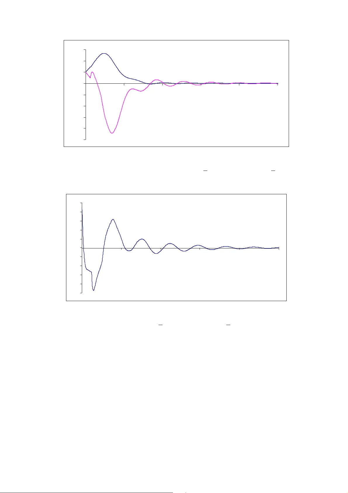
1 Predictor-Based Output Feedback for Nonlinear Delay Systems Iasson Karafyllis * and Miroslav Krstic ** * Dept. of Environmental Eng., Tec hnical University of Crete, 73100, Chania, Greece, email: ikarafyl@enveng.tuc.gr ** Dept. of Mechanical and Aerospace Eng., University of California, San Diego, La Jolla, CA 92093-0411, U.S.A., email: krstic@ucsd.edu Abstract We provide two solutions to the hereto fore open pr oblem of stabilization of systems with arbitrarily long delays at the input and output of a nonlinear system using output feedback only. Both of our solutions are global, employ the predictor approach over the peri od that combines th e input and output delays, address nonlinear systems with sa mpled measurements and with control applied using a zero-order hold, and require that the sampling/holding periods be sufficiently short, though not n ecessarily constant. Our first approach considers general nonlinear systems for which the solution map is available explicitly and whose one-sample-period predictor-based discrete-ti me model allows state reconstruction, in a finite number of steps, from the past values of inputs and output measurements. Our second approach considers a class of globally Lipschitz strict-feedback systems with dist urbances and employs an appropriately constructed successive a pproximation of the predictor map, a high-gain sampled-data observer, and a linear stabilizing feedback for the delay-free system. We specialize the sec ond approach to linear s ystems, where the predictor is available explicitly. We provide two i llustrative examples—one analytical for the first approach and one numerical for the second approach. Keywords: nonlinear systems, delay systems, sampled-data control. 1. Introduction Summary of Results of the Paper. Even though numerous results ha ve been developed in recent years for stabilization of nonlinea r systems with input delays by state feedback [18,20,24,25,26,27,30,31,32,46,50], and although add itional delays in state measurements are allow ed in our recent work [20] , the problem of stabilization of systems with arbitrarily long delays at the input and/or output by output feedback has remained open. We provide two solutions to this problem . Bo th of our solutions address nonlinear systems with sampled measurements and with control applied us ing a zero-order hold, with a requirement that the sampling/holding periods be su fficiently short, though not necessarily constant. Both of our solutions also em ploy the predictor approach to pr ovide th e control law with an estim ate of the future state over a period that comb ines the input and output delays. 2 Our first approach considers general nonlinea r system s for which the solution map is available explicitly and whose one-sampl e-period predicto r-based discrete-tim e model allows state reconstruction, in a finite number of steps, from the past values of inputs and output measurements. Our second approach considers a class of globally Lipschitz strict -feedback systems with disturbances and employs an appropriately constr ucted successive approximation of the predictor map, a high-gain sampled-data observer, and a li near stabilizing feedback for the delay-free system. The results of the second approach can be applied to the linear time-invariant case as well, providing robust global exponential sa mpled-data stabilizers, which ar e com pletely insensitive to perturbations of the sampling schedule. Both of our approaches achieve global as ymptotic stabilization. Th e first approach also achieves dead-beat stabilization in case the delay-free plant is d ead-beat stabilizable. The second approach achieves input-to-state stability with respect to plan t disturbances and m easurement disturbances, as well as global exponentia l stability in the absence of disturbances. Problem Statement and Literature. As in [18,20,24,25,26,27,50] we consider nonlinear system s of the form: m n U t u t x t u t x f t x ℜ ⊆ ∈ ℜ ∈ − = ) ( , ) ( )) ( ), ( ( ) ( τ  (1.1) where 0 ≥ τ is the input delay, m U ℜ ⊆ is a non-empty set with U ∈ 0 (th e control set) and n n U f ℜ → × ℜ : is a locally Lipschitz mapping with 0 ) 0 , 0 ( = f . We employ the predictor-based approach, which is ubiquitous for linear systems (see [40] and the refere nces in [25,26]) and is different from other approaches for systems w ith input delays [30,31,32,46], where the stabilizing feedback for the delay free system is either applie d or is m odified and stability is guaranteed for sufficiently small input delays. The input in (1.1) can be applied continuously or with zero-order hold (see [20]) and the measured output is usually assumed to be the state vector n t x ℜ ∈ ) ( . In [20], we extended predictor-based nonlin ear control to the case of sampled m easurements and measurement delays expressed as ) ( ) ( r x t y i − = τ , for ) , [ 1 + ∈ i i t τ τ where y is the measured output, th e discrete time instants i τ are the sampling times an d 0 ≥ r is the measurement delay. The m otivation is that sampling arises sim ultaneously with input and output delays in control over networks. Few papers have studied this problem (exceptions are [14] where input and measurem ent delays are considered for linear system s but the measurement is not sampled and [22] where th e unicycle is studied). In the absence of delays, in sampled-data control of nonlinear systems sem iglobal practical stability is generally guaranteed [10,35,36,37], with th e desired region of a ttraction achieved by sufficiently fast sampling. Altern atively, global results are achieved under re strictive conditions on the structure of the system [9,13,39]. Simultaneous consider ation to sampling and delays (either physical or sampling-indu ced) is given in the literature on control of linear and nonlinear systems over networks [7,8,12,37,39,44,45,49], but almost all available results rely on delay- dependent conditions for the existence of stabili zing feedback. Exceptions are the papers [3,28], where prediction-based contro l methodologies are em ployed. The assumption that the state vector is measur ed is s eldom realistic. Instead, measurement is a function of the state vector, i.e., the meas ured output of system (1.1) is given by: + ∈ + ∈ − = Z i T i iT t r iT x h t y ), ) 1 ( , [ )), ( ( ) ( 1 1 1 (1.2) 3 where 0 1 > T is the sampling period, 0 ≥ r is the m easurement delay and k n h ℜ → ℜ : is a continuous vector field with 0 ) 0 ( = h (the output map). Notice that the m easurements are obtained at discrete time instants. We study the following problem in this pape r: find a feed back law, which utilizes the sampled measurements and app lies the i nput with zero-order hold, given by j u t u = ) ( , + ∈ + ∈ Z j T j jT t , ) ) 1 ( , [ 2 2 (1.3) where 0 2 > T is the holding period, such that the clos ed-loop system (1.1) with (1.2), (1.3) is globally asymptotically stable. Two Solutions Provided in the Paper. The above problem is solved for two particular cases: 1 st Case (Section 2): The case where the soluti on map of the open-loop system (1.1) is explicitly known and 0 2 1 > = = T T T (sample-and-hold case). Under appropriate assumptions for observability, forward completeness and sampled- data stabilizability of the open loop system (1.1) with 0 = τ , we guarantee stabilization of system (1.1) with a pred ictor-based version of any sampled-data controller designed fo r the delay-free plant. For example, all sam pled-data feedback designs proposed in [9,10,13,21,35,36,37,39] which gua rantee global stabilization can be exploited for the stabilization of a delayed system with input/measurem ent delays, sampled measurements and input applied with zero orde r hold. The class of feedforward systems (see [23,26] and references therein) can be addressed by using the pr oposed observer-based predictor feedback design. 2 nd Case (Sections 3,4 and 5): The class of globally Lipschitz systems of the form n n n n n n n n i i i i i i t d t d t d t u t x t x t x t u t d t u t x g t x f t x n i t d t u t x g t x t x t x f t x ℜ ∈ ′ = ℜ ∈ ℜ ∈ ′ = − + + = − = + + = + ) ) ( ),..., ( ( ) ( , ) ( , ) ) ( ),..., ( ( ) ( ) ( ) ( )) ( ), ( ( )) ( ( ) ( 1 ,..., 1 , ) ( )) ( ), ( ( ) ( )) ( ),..., ( ( ) ( 1 1 1 1 τ   (1.4) where ℜ → ℜ i i f : ( n i ,..., 1 = ) are globally Lipschitz functions with 0 ) 0 ( = i f ( n i ,..., 1 = ) and the output map is 1 ) ( x x h = . The inputs i d ( n i ,..., 1 = ) represent disturbances and the functions ℜ → ℜ i i g : ( n i ,..., 1 = ) are locally Lipschitz, bounded functi ons. In this case, we can show stabilizability of system (1.1) even under arbitrary perturbations of the sampling schedule, by combining the sampled-data observer design in [17] and the approxim ate predictor control proposed in [18]. We also show robustness with respect to measurement errors and modeling errors. The feedback design is base d on the corresponding delay free system ) ( )) ( ( ) ( 1 ,..., 1 , ) ( )) ( ),..., ( ( ) ( 1 1 t u t x f t x n i t x t x t x f t x n n i i i i + = − = + = +   (1.5) The proposed control schemes for both cases consist of three com ponents: 1 st Component: An observer, which utilizes past inpu t and output values in order to provide (continuous or discrete) estimates of the delayed state vector ) ( r t x − . 2 nd Component: The predictor mapping that u tilizes the estimation provided by the observer and past input values in order to provide an estim ation of the future value of the state vector ) ( τ + t x . 4 3 rd Component: A nominal globally stabilizing feedback for the corresponding delay-free system. The above control scheme has long been in us e for linear systems [ 29,33,34,48,51] and it has been used even for partial differential equation sy stems [11], but is novel for nonlinear system s. Moreover, even for Linear Time-Invarian t (LTI) systems ) ( ) ( ) ( ) ( t Gd t Bu t Ax t x + − + = τ  (1.6) where n n t d t u t x ℜ ∈ ℜ ∈ ℜ ∈ ) ( , ) ( , ) ( , we provide new sampled-data feedback exponential stabilizers that are robust to perturbations of the sampling schedule. Notation. Throughout the paper we adopt the following notation: ∗ For a vector n x ℜ ∈ we denote by x its usual Euclidean norm, by x ′ its transpose. For a real matrix m n A × ℜ ∈ , n m A × ℜ ∈ ′ denotes its transpose and { } 1 , ; sup : = ℜ ∈ = x x Ax A n is its induced norm. n n I × ℜ ∈ denotes the identity matrix. By ) ,..., , ( diag 2 1 n l l l A = we mean a diagonal matrix with n l l l ,..., , 2 1 on its diagonal. ∗ + ℜ denotes the set of non-negative real numbers. + Z denotes the set of non-negative integers. For every 0 ≥ t , [] t denotes the integer part of 0 ≥ t , i.e., the largest integer being less or equal to 0 ≥ t . A partition {} ∞ = = 0 i i T π of + ℜ is an increasing sequence of times with 0 0 = T and + ∞ → i T . ∗ We say that an incr easing continuous function + + ℜ → ℜ : γ is of class K if 0 ) 0 ( = γ . We say that a function γ of class K i s o f c l a s s ∞ K if + ∞ = +∞ → ) ( lim s s γ . By K L we denote the set of all continuous functions + + + ℜ → ℜ × ℜ : σ with the properties: (i) for each 0 ≥ t the mapping ) , ( t ⋅ σ is of class K ; (ii) for each 0 ≥ s , the mapping ) , ( ⋅ s σ is non-increasing with 0 ) , ( lim = +∞ → t s t σ . ∗ By ) ( A C j ( ) ; ( Ω A C j ), where n A ℜ ⊆ ( m ℜ ⊆ Ω ), 0 ≥ j is a non-negative integer, we denote the class of functions (taking values in m ℜ ⊆ Ω ) that have continuous derivatives of order j on n A ℜ ⊆ . ∗ Let n b r a x ℜ → − ) , [ : with 0 ≥ > a b and 0 ≥ r . By x t T r ) ( we denote the “history” of x from r t − to t , i.e., () ] 0 , [ ; ) ( : ) ( ) ( r t x x t T r − ∈ + = θ θ θ , for ) , [ b a t ∈ . By x t T r ) (  we denote the “open history” of x from r t − to t , i.e., ( ) ) 0 , [ ; ) ( : ) ( ) ( r t x x t T r − ∈ + = θ θ θ  , for ) , [ b a t ∈ . ∗ Let ℜ ⊆ I be an interval. By ) ; ( U I ∞ L ( ) ; ( U I loc ∞ L ) we denote the space of measurable and (locally) bounded functions ) ( ⋅ u defined on I and taking values in m U ℜ ⊆ . Notice that we do not identify functions in ) ; ( U I ∞ L which differ on a measure zero set. For ) ]; 0 , ([ n r x ℜ − ∈ ∞ L or ) ); 0 , ([ n r x ℜ − ∈ ∞ L we define ) ( sup : ] 0 , [ θ θ x x r r − ∈ = or ) ( sup : ) 0 , [ θ θ x x r r − ∈ = . Notice that ) ( sup ] 0 , [ θ θ x r − ∈ is not the essential supremum but the actual s upremum and that is why the quantities ) ( sup ] 0 , [ θ θ x r − ∈ and ) ( sup ) 0 , [ θ θ x r − ∈ do not coincide in general. ∗ The saturation function ) ( x sat is defined by x x x sat / ) ( = for all ℜ ∈ x . Throughout the paper, for 0 = r we adopt the convention n n r ℜ = ℜ − ∞ ) ]; 0 , ([ L and n n r C ℜ = ℜ − ) ]; 0 , ([ 0 . Finally, for reader’s convenience, we mention the following fact, which is a 5 direct consequence of Lemma 2.2 in [1] and Lemma 3.2 in [15]. The fact is used extensively throughout the paper. FACT: Suppose that the system )) ( ), ( ( ) ( t u t x f t x =  is forward complete. Then for every n x ℜ ∈ 0 , ) ); , ([ m loc u ℜ +∞ − ∈ ∞ τ L , the solution ) ( t x of (1.1) with initial condition n x x ℜ ∈ = 0 ) 0 ( and corresponding to input ) ); , ([ m loc u ℜ +∞ − ∈ ∞ τ L exists for all 0 ≥ t . Moreover, for every 0 > T there exists a function ∞ ∈ K a such that for every n x ℜ ∈ 0 , ) ); , ([ m loc u ℜ +∞ − ∈ ∞ τ L the solution ) ( t x of (1.1) with initial condition n x x ℜ ∈ = 0 ) 0 ( and corresponding to input ) ); , ([ m loc u ℜ +∞ − ∈ ∞ τ L satisfies ⎟ ⎠ ⎞ ⎜ ⎝ ⎛ + ≤ − < ≤ − ) ( sup ) ( 0 s u x a t x t s τ τ , for all ] , 0 ( T t ∈ . 2. Solution Map Known Explicitly We consider system (1.1) under the following hypotheses: Hypothesis (H1): The system m n U t u t x t u t x f t x ℜ ⊆ ∈ ℜ ∈ = ) ( , ) ( , )) ( ), ( ( ) (  (2.1) is forward complete. Hypothesis (H2): There exists U k n → ℜ : , ∞ ∈ K a such that the n ℜ ∈ 0 is Globally Asymptotically Stable for the closed-l oop system (2.1) with + ∈ + ∈ = Z i T i iT t iT x k t u ), ) 1 ( , [ )), ( ( ) ( (2.2) i.e., there exists KL ∈ σ such that for every 0 ≥ t , n x ℜ ∈ 0 , the solution ) ( t x of the closed-loop system (2.1) with (2.2) at time 0 ≥ t with initial condition n x x ℜ ∈ = 0 ) 0 ( exists and satisfies ( ) t x t x , ) ( 0 σ ≤ . Moreover, the following inequality holds: ( ) x a x k ≤ ) ( , n x ℜ ∈ ∀ (2.3) Let ) ; , ( 0 u x t φ denote the solution map of (2.1), i.e., the unique solution n t x ℜ ∈ ) ( of (2.1) at time 0 ≥ t with initial condition n x x ℜ ∈ = 0 ) 0 ( and corresponding to a measurable and essentially bounded input U t u → ] , 0 [ : satisfies ) ; , ( ) ( 0 u x t t x φ = . The control approach that we will use for the stabilization of system (1.1) assumes explicit knowledge of the solution map ) ; , ( 0 u x t φ of (2.1). If the output map were the identity f unction then the ap proach in [20] could be directly a pplied for the stabilization of (1.1). Here, we need an additional observability hypothesis. Let + ∈ Z l be an integer such that δ τ + = + T l r , where ) , 0 [ T ∈ δ . If 0 > δ , then we can define the operator () U T U P ); , 0 [ : 2 ∞ → L by means of the formula () 1 2 1 : ) ( ) , ( u t u u P = , for ) , 0 [ δ ∈ t and ( ) 2 2 1 : ) ( ) , ( u t u u P = , for ) , [ T t δ ∈ 6 and the mapping n n U F ℜ → × ℜ 2 : by means of the equation: ( ) ) , ( ; , : ) , , ( 2 1 2 1 u u P x T u u x F φ = (2.4) Notice that the previous defin itions in conjunction with the se migroup property for the solution map, imply for all + ∈ Z i with 1 + ≥ l i : ) , ), ( ( ) ) 1 (( 2 1 u u r iT x F r T i x − = − + (2.5) where ) ( t x denotes any solution of (1.1) with pi ecewise constant input that satisfies () ) ( ) , ( ) ( 2 1 θ θ τ u u P r iT u = + − − for all ) , 0 [ T ∈ θ . If 0 = δ then we similarly define the operator ( ) U T U P ); , 0 [ : ∞ → L by means of the formula () u t u P = : ) ( ) ( , for ) , 0 [ T t ∈ and the mapping n n U F ℜ → × ℜ : by means of the equation: ( ) ) ( ; , : ) , ( u P x T u x F φ = (2.6) Notice again that the previous definitions in conjunction with the semigroup property for the solution map, give for all + ∈ Z i with l i ≥ : ) ), ( ( ) ) 1 (( u r iT x F r T i x − = − + (2.7) where ) ( t x denotes any solution of (1.1) with constant input that satisfies u T l i u ≡ + − ) ) (( θ . Therefore for every ) , 0 [ T ∈ δ , we can construct an autonomous di screte-time system of the form )) ( ( ) ( ) ( , ) ( , )) ( ), ( ( ) 1 ( i x h i y V i v i x i v i x F i x n = ∈ ℜ ∈ = + (2.8) which is associated with system (1.1), (1.2) and represents a one-sa mpling-period “predictor system”. Notice that 2 U V = for the case 0 > δ and U V = for the case 0 = δ . The following observability hypothesis is employed in the present work (see also [16]). Hypothesis (H3): The discrete-time system (2.8) is completely observable, i. e., there exists + ∈ Z p , 1 ≥ p and a continuous function n k kp p V ℜ → ℜ × ℜ × Ψ : with 0 ) 0 , 0 ( = Ψ such that the solution of the discrete-time system (2.8) with arbitrary initial condition corresponding to arbitrary input satisfies )) ( ),..., ( ), 1 ( ),..., ( ( ) ( p i y i y p i v i v p i x + − + Ψ = + for all + ∈ Z i . Example 2.1: We consider the 3-dimensional feedforward system ℜ ⊆ ∈ ℜ ∈ ′ = + = − + = − = U u x x x x t x t x t x t u t x t x t x t u t x , ) , , ( ) ( ) ( ) ( , ) ( ) ( ) ( ) ( , ) ( ) ( 3 3 2 1 2 1 2 3 1 1 2 1    τ τ (2.9) This system (for 0 = τ ) is not feedback lineari zable [23]. Hypothesis (H1) holds for system (2.9) and its solution map with 0 = τ is given by: 7 () () ∫∫ ∫∫ ∫∫∫ ∫ ∫∫ ∫ ⎟ ⎟ ⎠ ⎞ ⎜ ⎜ ⎝ ⎛ + + + + + + + = + + + + = + = tw t tw t t t dw ds s u t x d ds s u x dw d ds s u u x t t x x u x t ds s u x d ds s u u x t x u x t ds s u x u x t 0 2 0 2 1 00 1 000 1 2 2 3 3 0 1 00 1 2 2 0 1 1 ) ( ) ( 3 ) ( ) ( 1 2 ) ; , ( ) ( ) ( ) ( 1 ) ; , ( ) ( ) ; , ( τ τ τ τ τ τ φ τ τ φ φ (2.10) Here we study the case ) , 0 ( T r ∈ + τ , in which the equality δ τ + = + T l r holds with τ δ + = r , 0 = l and the mapping 3 2 3 : ℜ → ℜ × ℜ F defined by (2.4) is given by () ) , ( ) , ( 3 2 ) , , ( ) , ( ) , ( ) , , ( ) , ( ) , , ( 2 1 3 2 1 2 1 1 2 2 1 2 3 2 1 3 2 1 2 2 1 1 1 1 2 2 1 2 2 1 1 1 2 1 1 u u G u u Q x x T x x T x u u x F u u G u u Q x x T x u u x F u u Q x u u x F + + + + + = + + + = + = (2.11) for all 2 2 1 ) , , ( U u u x n × ℜ ∈ , where ℜ → ℜ 2 3 2 2 1 : , , , G G Q Q are defined by: 2 ) ( 2 ) ( 3 3 2 2 3 6 ) ( 3 2 ) , ( 2 ) ( ) ( 2 ) , ( ) , ( 2 ) ( ) ( 2 : ) , ( ) ( : ) , ( 3 2 2 2 2 1 2 1 2 3 2 1 2 2 2 1 3 2 2 2 2 1 2 1 2 2 1 2 2 1 2 2 2 1 1 2 2 1 2 2 1 2 1 1 δ δ δ δ δ δ δ δ δ δ δ δ δ δ δ δ δ δ δ − + − + ⎟ ⎠ ⎞ ⎜ ⎝ ⎛ − + − + ⎥ ⎥ ⎦ ⎤ ⎢ ⎢ ⎣ ⎡ + − = − + − + + = − + − + = − + = T u T u u u T T u u T T u u G u T u u T u u u Q u u G u T u T u u u Q u T u u u Q We consider two cases: 1 st Case (two states are measured): ℜ ⊆ U with U ∈ 0 is arbitrary and the m easured output of (2.9) is given by (1.2), where ) , ( ) ( ) , ( 3 1 2 1 ′ = = ′ = x x x h y y y (2.12) In this case, system (2.8) is com pletely observable with 1 = p , since the solution of the discrete- time system (2.8) with arbitrar y initial condition and corresponding to arbitr ary input satisfies () ⎥ ⎥ ⎥ ⎦ ⎤ ⎢ ⎢ ⎢ ⎣ ⎡ + + + − − + + = + − ) 1 ( )) ( ), ( ( )) ( ), ( ( ) ( ) ( ) ( ) 1 ( ) 1 ( ) 1 ( 2 2 1 2 1 1 2 1 2 2 1 1 i y i u i u C i u i u B i y i y i y i y T i y i x (2.13) where ) , ( ) , ( ) , ( , 2 ) , ( ) , ( 3 ) , ( 2 1 3 1 2 1 2 2 1 2 1 1 2 1 2 1 2 1 u u G T u u G u u C T u u Q u u Q T u u B − − − = + + − = 2 nd Case (only one state is measured): ] , [ ε ε − ⊆ U with U ∈ 0 , ⎟ ⎠ ⎞ ⎜ ⎝ ⎛ ∈ 6 1 , 0 ε and the measured output of (2.9) is given by (1.2), where 3 ) ( x x h y = = (2.14) 8 In this case the following equation h olds for all + ∈ Z i for the solution of the discrete-time system (2.8), where 3 2 3 : ℜ → ℜ × ℜ F is defined by (2.11): () ) ( )) ( ), ( ( 3 )) 1 ( ), 1 ( ( 3 )) ( ), ( ( 3 )) 1 ( ), 1 ( ), ( ), ( ( ) ( ) 1 ( 2 ) 2 ( 1 2 1 2 2 1 2 2 1 1 2 2 1 2 1 3 3 3 i x i u i u Q i u i u Q i u i u TQ T i u i u i u i u P i x i x i x − + + + + = + + − + + − + where ( ) ) , ( ) , ( ) , ( 6 2 1 ) , ( ) , ( ) , ( : ) , , , ( 2 1 2 1 2 1 1 2 1 2 2 2 1 2 2 1 3 2 1 3 2 1 2 1 u u TQ u u Q v v Q T u u TG u u G v v G v v u u P − + − + − = . The above definitions 2 1 2 1 1 ) ( : ) , ( u T u u u Q δ δ − + = , 2 2 1 1 2 2 1 2 2 ) ( ) ( 2 : ) , ( u T u T u u u Q δ δ δ δ − + − + = show that if ] , [ ε ε − ⊆ U with ⎟ ⎠ ⎞ ⎜ ⎝ ⎛ ∈ 6 1 , 0 ε then the inequalities ε 2 ) , ( 2 2 1 2 T u u Q ≤ , ε T u u Q ≤ ) , ( 2 1 1 hold for all U u u ∈ 2 1 , . Therefore the inequality 2 2 1 2 2 1 2 2 1 1 2 ) 6 1 ( )) ( ), ( ( 3 )) 1 ( ), 1 ( ( 3 )) ( ), ( ( 3 T i u i u Q i u i u Q i u i u TQ T ε − ≥ − + + + + holds for all U i u i u ∈ ) ( ), ( 2 1 , U i u i u ∈ + + ) 1 ( ), 1 ( 2 1 . In this case, system (2.8) is completely observable with 2 = p , since the solution of the discrete-time sy stem (2.8) with arbitrary ini tial condition and corresponding to arbitrary input satisfies () )) ( ), ( ( )) 1 ( ), 1 ( ), ( ), ( ( )) 1 ( ), 1 ( ), ( ), ( ( ) ( ) 1 ( 2 ) 2 ( ) 2 ( )) 1 ( ), 1 ( ( )) 1 ( ), 1 ( ( ) 1 ( ) 2 ( )) 1 ( ), 1 ( ( ) 2 ( 2 1 1 2 1 2 1 2 1 2 1 2 1 2 1 2 1 2 1 1 i u i u Q i u i u i u i u D i u i u i u i u P i y i y i y M i y i u i u C i u i u B M M i y i y T i u i u Q M i x + + + + + − + + − + = ⎥ ⎥ ⎥ ⎦ ⎤ ⎢ ⎢ ⎢ ⎣ ⎡ + + + + + + + − + − + + + + = + − (2.15) where ) , ( 3 ) , ( 3 ) , ( 3 : ) , , , ( 2 1 2 2 1 2 2 1 1 2 2 1 2 1 u u Q v v Q u u TQ T v v u u D − + + = .  Next, we consider again the genera l system (1.1), (1.2), (1.3) with 0 2 1 > = = T T T . By virtue of hypothesis (H1) the solution of ( 1.1), (1.2), (1.3) exists for all 0 ≥ t for arbitrary initial c ondition ( ) n r r C x x T ℜ − ∈ = ]; 0 , [ ) 0 ( 0 0 , ( ) U u T ); 0 , [ ) 0 ( τ τ − ∈ ∞ L  and arbitrary sequence of inputs ∞ = 0 } { i i u . The measurements m ade up to time iT t = are given by ) ) 1 ( , [ )), ( ( ) ( T j jT t r jT x h y t y j + ∈ − = = for i j ,..., 0 = . Notice that, if we denote ) ( r jT x x j − = for all + ∈ Z j with τ + ≥ r jT , then we obtain ) , , ( 1 1 l j l j j j u u x F x − − − + = for the case 0 > δ and ) , ( 1 l j j j u x F x − + = for the case 0 = δ , where F is defined by (2.4) or (2.6) and + ∈ Z l is the integer such tha t δ τ + = + T l r , where ) , 0 [ T ∈ δ . Hypothesis (H3) implies the exis tence of a continuous function n k kp p U R ℜ → ℜ × ℜ × + 1 : (called the reconstruction mapping) for the case 0 > δ and n k kp p U R ℜ → ℜ × ℜ × : for the case 0 = δ with 0 ) 0 , 0 ( = R such that for every + ∈ Z i with T l p iT ) 1 ( + + ≥ , the following equality holds: ) ,..., , ,..., ( ) ( 1 1 i p i l i l p i i y y u u R r iT x x − − − − − − = − = , for the case 0 > δ (2.16) ) ,..., , ,..., ( ) ( 1 i p i l i l p i i y y u u R r iT x x − − − − − = − = , for the case 0 = δ (2.17) We are also in a position to define the predictor mapping that correlates ) ( r iT x − with ) ( τ + iT x , which is given by ( ) ) ,..., ( ; , : ) ,..., , ( 1 1 1 1 − − − − − − + = Φ i l i i l i u u Q x r u u x τ φ , for the case 0 > δ (2.18) ( ) ) ,..., ( ; , : ) ,..., , ( 1 1 − − − − + = Φ i l i i l i u u Q x r u u x τ φ , for the case 0 = δ (2.19) where 9 () 1 1 1 : ) ( ) ,..., ( − − − − − = l i i l i u t u u Q , for ) , 0 [ δ ∈ t , () j i l i u t u u Q = − − − : ) ( ) ,..., ( 1 1 , ) ) 1 ( , ) [( δ δ + − + + + − + ∈ T i l j T i l j t , 1 ,..., − − = i l i j for the case 0 > δ and for the case 0 = δ () j i l i u t u u Q = − − : ) ( ) ,..., ( 1 , for ) ) 1 ( , ) [( T i l j T i l j t − + + − + ∈ , 1 ,..., − − = i l i j By virtue of (2.16), (2.17), (2.18) and ( 2.19) the following equali ties hold for every + ∈ Z i with 1 + + ≥ l p i : ( ) 1 1 1 1 ,..., ), ,..., , ,..., ( ) ( − − − − − − − − − Φ = + i l i i p i l i l p i u u y y u u R iT x τ , for the case 0 > δ (2.20) ( ) 1 1 ,..., ), ,..., , ,..., ( ) ( − − − − − − − Φ = + i l i i p i l i l p i u u y y u u R iT x τ , for the case 0 = δ (2.21) The computation of the predictor mapping and the reconstruction mapping is straightforward when the solution map of (2.1) is known. The following example illustrates how easily th e prediction and reconstruction mappings can be computed. Example 2.2: We return to Example 2.1 and consider th e 3-dim ensional feedforward system (2.9) with output defined by (2.14), ] , [ ε ε − ⊆ U with U ∈ 0 , ⎟ ⎠ ⎞ ⎜ ⎝ ⎛ ∈ 6 1 , 0 ε , for the case ) , 0 ( T r ∈ + τ . In this case the equality δ τ + = + T l r holds with τ δ + = r , 0 = l and the mapping 3 2 3 : ℜ → ℜ × ℜ F defined by (2.4) is given by (2.11). In order to define the reconstruction mapping 3 2 3 : ℜ → ℜ × ℜ × U R we simply need to replace ) ( ), 1 ( ), 2 ( i y i y i y + + by 2 1 , , − − i i i y y y , respectively, to use equation (2.15) with ) 1 ( ) ( 1 2 + = i u i u and to replace ) ( ), ( ), 1 ( 1 2 2 i u i u i u + by 3 2 1 , , − − − i i i u u u , resp ectively. Therefore, we obtain: () ) , ( ) , , , ( ) , , , ( 2 ) , ( ) , ( ) , ( : ) , , , , , ( 2 3 1 1 2 2 3 1 2 2 3 2 1 1 2 1 2 2 1 1 1 2 1 1 2 1 2 3 − − − − − − − − − − − − − − − − − − − − − − − − − + − + − = ⎥ ⎥ ⎥ ⎦ ⎤ ⎢ ⎢ ⎢ ⎣ ⎡ + + − − + = i i i i i i i i i i i i i i i i i i i i i i i i i i i i u u Q u u u u D u u u u P y y y M y u u C u u B M M y y T u u Q M y y y u u u R (2.22) where the mappings D P C B Q , , , , 1 have been defined in Example 2.1. The predictor mapping is simply obtained from (2.10): () () 2 1 3 1 1 2 1 3 1 2 2 1 2 3 1 3 1 1 1 1 2 1 2 1 2 1 1 1 1 2 2 3 6 2 ) , ( 1 2 ) , ( ) , ( − − − − − − − − − − + + + + + + = Φ + + + + = Φ + = Φ i i i i i i i i i i u u x u x x x x u x u x u u x x u x u x u x δ δ δ δ δ δ δ δ δ (2.23) In general, the rule to obtain the reconstruction mapping from the mapping n k kp p V ℜ → ℜ × ℜ × Ψ : for the case 0 > δ involved in Hypothesis (H3) is to replace V j i u j i u j i v ∈ + + = + )) ( ), ( ( ) ( 2 1 by ) , ( 1 j l p i j l p i u u + − − + − − − for 1 ,..., 0 − = p j (notice that 2 U V = ) and ) ( j i y + by j p i y + − for 1 ,..., 0 − = p j .  In summary, the proposed control sche me consists of three com ponents: 1 st Component: A sampled-data observer based on a state-reconstruction mapping n k kp p U R ℜ → ℜ × ℜ × + 1 : , given by (2.16) for the discrete -time one-sam ple-period “predictor 10 system” (2.8). The reconstruction mapping utilizes past input and output valu es in order to provide an estimate for the delayed state vecto r ) ( r iT x − . 2 nd Component: The predictor mapping Φ , given by (2.20), which utilizes the estimation provided by the reconstruction map and past input values in order to provide an estimation of the future value of the state vector ) ( τ + iT x . 3 rd Component: The nominal globally stabilizing feedback U k n → ℜ : involved in Hypothesis (H2), which employs the predictor. We are now ready to state our main resu lt. Its proof is provided in the Appendix. Theorem 2.3: Let 0 > T , 0 , ≥ τ r with 0 > + τ r be given and let + ∈ Z l and ) , 0 ( T ∈ δ be such that δ τ + = + T l r . Moreover, suppose that Hypotheses (H1)-( H3) hold for system (1.1) , (1.2) with T T T = = 2 1 . Then the closed-loop system (1.1), (1.2), (1.3) with ( ) ) ,..., , ( ) ( 1 1 − − − Φ = i l i u u X k t u , for ) ) 1 ( , [ T i iT t + ∈ (2.24) where ) ( jT u u j = and ) ,..., , ,..., ( 1 1 i p i l i l p i y y u u R X − − − − − − = (2.25) where )) ( ( r jT x h y j − = , is Globally Uniformly Asymptotically St able, in the sense that there exists a function KL ∈ σ ~ such that for every ( ) U T l p pT r C u x n ); 0 , ) 1 ( [ ) ]; 0 , ([ ) , ( 0 0 0 + + − × ℜ − − ∈ ∞ L , the solution m n t u t x ℜ × ℜ ∈ )) ( ), ( ( of the closed-loop system (1.1), (1.2), (1.3) , ( 2.24), (2.25) with T T T = = 2 1 , initial condition () U T l p u u T r ); 0 , ) 1 ( [ ) 0 ( 0 + + − ∈ = ∞ + L τ  , ( ) n r pT r C x x T ℜ − − ∈ = ]; 0 , [ ) 0 ( 0 0 satisfies the following inequality for all 0 ≥ t : ( ) t u x u t T x t T T l p pT r T l p T l p pT r pT r , ~ ) ( ) ( ) 1 ( 0 0 ) 1 ( ) 1 ( + + + + + + + + + + ≤ + σ  (2.26) Finally, if the closed-loop syst em (2.1), (2.2) satisfies the dead-beat property of order jT , where + ∈ Z j is positive, i.e., for all n x ℜ ∈ 0 the solution ) ( t x of (2.1), (2.2) wit h initial condition n x x ℜ ∈ = 0 ) 0 ( satisfies 0 ) ( = t x for all jT t ≥ , then there exists + ∈ Z q such that the closed-loop system (1.1), (1.2), (1.3), (2.24), (2.25) satisfies the dead-beat property of order qT , i.e., for every () U T l p pT r C u x n ); 0 , ) 1 ( [ ) ]; 0 , ([ ) , ( 0 0 0 + + − × ℜ − − ∈ ∞ L , the solution m n t u t x ℜ × ℜ ∈ )) ( ), ( ( of system (1.1), (1.2), (1.3), (2.24), ( 2.25) with init ial condition () U T l p u u T r ); 0 , ) 1 ( [ ) 0 ( 0 + + − ∈ = ∞ + L τ  , ( ) n r pT r C x x T ℜ − − ∈ = ]; 0 , [ ) 0 ( 0 0 satisfies 0 ) ( = t x for all qT t ≥ . Remark 2.4: A very sim ilar statement holds for the case 0 = δ . The only thing th at needs to be changed is the feedback law (2.24), (2.25), which is replaced by () ) ,..., , ( ) ( 1 − − Φ = i l i u u X k t u , for ) ) 1 ( , [ T i iT t + ∈ and ) ,..., , ,..., ( 1 i p i l i l p i y y u u R X − − − − − = . Example 2.5: We return to Example 2.2 and consider th e 3-dim ensional feedforward system (2.9) with output defined by (2.14), ] , [ ε ε − = U with ⎟ ⎠ ⎞ ⎜ ⎝ ⎛ ∈ 6 1 , 0 ε , for the case ) , 0 ( T r ∈ + τ . In this case the equality δ τ + = + T l r holds with τ δ + = r , 0 = l . It is shown in [21] (Theorem 3.7 and Remark 3.8) 11 that Hypothesis (H2) holds for system (2.9) for every 0 > ε . More specifically, for every 0 > ε there exist constants 0 , , , , , 2 1 2 1 0 > T R R K K K such that hypothesis (H2) holds with () () () () () ⎪ ⎪ ⎪ ⎩ ⎪ ⎪ ⎪ ⎨ ⎧ < + + ⎟ ⎠ ⎞ ⎜ ⎝ ⎛ + + − + − ≥ + + < + − − ≥ + + ≥ − = 2 2 2 1 2 2 1 2 3 2 2 1 2 2 2 1 2 2 1 1 1 2 1 1 2 2 2 1 2 2 1 1 1 0 2 1 sat 2 sat ) ( sat : ) ( R x x x if x x x K x x R x x x and R x if x x K x R x x x and R x if x K x k (2.27) Moreover, the inequality ε ≤ ) ( x k holds for all 3 ℜ ∈ x . It follows from Theorem 2.3 that the closed-loop system (2.9), ( 1.2), (2.24), (2.25), where Φ , , R h are defined by ( 2.14), (2.22), (2.23), respectively, is Globally Uniforml y Asymptotically Stable in the sense described in Theorem 2.3. For the case where U ⊆ − ] , [ ε ε and the output map is given by ( 2.12) (the case where two states are measured), we showed in Example 2.1 that Hypot hesis (H3) holds. It follows from Theorem 2.3 that the closed-loop syst em (2.9), (1.2) with ) ) 1 ( , [ ), ˆ ( ) ( T i iT t X k t u + ∈ = , where ℜ → ℜ 3 : k is defined by (2.27), ) ˆ , ˆ , ˆ ( ˆ 3 2 1 ′ = X X X X , () () () 2 1 3 1 1 2 1 1 3 1 2 2 1 2 3 3 1 1 1 1 2 1 2 2 1 1 1 3 ) ( 2 ) ( 3 1 6 ) ( 2 ) ( ) ( ˆ ) ( 1 2 ) ( ) ( ˆ ) ( ˆ − − − − − − − − + + + + + + + + + + + + = + + + + + + + = + + = i i i i i i i i u r X u r u u r X r X X r X X X u r u u r X r X X u r X X τ τ τ τ τ τ τ τ τ (2.28) where ) ) 1 (( 1 T i u u i − = − and ) , , ( 3 2 1 ′ = X X X X is defined by () ⎥ ⎥ ⎥ ⎦ ⎤ ⎢ ⎢ ⎢ ⎣ ⎡ + − + − − − − = − − − − − ) ( ) , ( ) , ( ) 1 ( ) 1 ( ) 1 ( ) ( ) ( 2 1 2 1 2 1 2 1 2 2 1 1 i y u u C u u B i y i y i y i y T i y X i i i i (2.29) where ) ( ) ( 1 1 r jT x j y − = , ) ( ) ( 3 2 r jT x j y − = , i i j , 1 − = , ) ) 2 (( 2 T i u u i − = − and the functions ℜ → ℜ 2 : , C B are defined in Example 2.1, is Globally Uniformly Asym ptotically Stable.  3. Globally Lipschitz Systems We consider system (1.4) with output ) ( ) ( ) ( 1 i i i r x y τ ξ τ τ + − = , + ∈ Z i (3.1) where ∞ = 0 } { i i τ is a partition of + ℜ with ( ) 1 1 0 sup T i i i ≤ − + ≥ τ τ . We assume that 0 > + τ r , where 0 ≥ r is the measurement delay and 0 ≥ τ is the input delay. The locally bounded input ℜ → ℜ + : ξ represents the measurement error and the m easurable and locally essent ially bounded inputs ℜ → ℜ + : i d ( n i ,..., 1 = ) represent disturbances. We assu me that there exist cons tants 0 ≥ L and 0 ≥ G such that ) ,..., ( ) ,..., ( ) ,..., ( 1 1 1 1 i i i i i i z x z x L z z f x x f − − ≤ − , i i x x ℜ ∈ ∀ ) ,..., ( 1 , i i z z ℜ ∈ ∀ ) ,..., ( 1 (3.2) 12 G u x g i ≤ ) , ( , ℜ × ℜ ∈ ∀ n u x ) , ( (3.3) for all n i ,..., 1 = . Moreover, 0 ) 0 ( = i f for all n i ,..., 1 = . Define n n x f x f x f ℜ ∈ ′ = ) ) ( ),..., ( ( : ) ( 1 1 , n n j i n j i a A × ℜ ∈ = = } ,..., 1 , : { , with 1 1 , = + i i a for all 1 ,..., 1 − = n i and 0 , = j i a if 1 + ≠ i j , n b ℜ ∈ ′ = ) 1 , 0 ,..., 0 ( , n c ℜ ∈ ′ = ) 0 ,..., 0 , 1 ( : . We notice that inequalities (3.2), (3.3) guarantee that system (1.4) is forward complete, i.e., for every ( ) ( ) n loc loc n d u x ℜ ℜ × ℜ +∞ − × ℜ ∈ + ∞ ∞ ; ); , [ ) , , ( 0 L L τ the solution n t x ℜ ∈ ) ( of system (1.4) with initial condition n x x ℜ ∈ = 0 ) 0 ( and corresponding to inputs () ( ) n loc loc d u ℜ ℜ × ℜ +∞ − ∈ + ∞ ∞ ; ); , [ ) , ( L L τ exists for all 0 ≥ t . Indeed, notice that the function 2 ) ( 2 1 ) ( t x t P = satisfies () ) ( 2 1 ) ( 2 1 ) ( 3 ) 1 ( ) ( 2 2 2 τ − + + + + ≤ t u t d G t P L n t P  , for almost a ll 0 ≥ t for which the solution n t x ℜ ∈ ) ( of system (1.4) exists. In tegrating the previous differe ntial inequality and using a standard contradiction argument, we conclude that the solu tion n t x ℜ ∈ ) ( of system (1.4) exists for all 0 ≥ t and satisfies the following estim ate for all 0 > t : ⎟ ⎠ ⎞ ⎜ ⎝ ⎛ + + ⎟ ⎟ ⎟ ⎠ ⎞ ⎜ ⎜ ⎜ ⎝ ⎛ + + + + ≤ − < ≤ − < ≤ t L n L n s u s d G x t x t s t s 2 3 ) 1 ( exp 3 ) 1 ( ) ( sup ) ( sup ) ( 0 0 τ τ (3.4) The proposed observer/predictor-based feedback law consists of three components: 1) A high-gain sampled-data observer for syst em (1.4), (3.1) which provides an estimate n t z ℜ ∈ ) ( of the delayed state vector ) ( r t x − . 2) An approximate predictor, i.e., a mapping that utilizes the applied input values and the estimate n t z ℜ ∈ ) ( provided by the observer in orde r to provide an estim ate for ) ( τ + t x . 3) A stabilizing feedback law for the delay-free system, i.e., system (1.5). In what follows, we are going to describe the construction of each on e of the components. We also assume that the input and m easurement delay values 0 , ≥ r τ are perfectly known (see Remark 3.7(a) below for the case where the measur ement delay is not precisely known). 1 st Component (High-Gain Sam ple-Data Observer): Let n n p p p ℜ ∈ ′ = ) ,..., ( 1 be a vector such that the matrix n n c p A × ℜ ∈ ′ + ) ( is Hurwitz. The existence of a vector n n p p p ℜ ∈ ′ = ) ,..., ( 1 is guaranteed, since the pair of matrices ) , ( c A is observable. The proposed high-gain sample-data observer is of the form: 0 , )) ( exp( ) ( ) ( ) ( ) ( ) , [ , ) ( )) ( ( ) ( ) ( )) ( ) ( ( )) ( ),..., ( ( ) ( 1 ,..., 1 , )) ( ) ( ( ) ( )) ( ),..., ( ( ) ( 0 1 1 1 1 1 1 1 1 2 1 1 1 1 1 = − + = + − = = ∈ + = − − + − ′ + = − = − ′ + + = + + + + + + + τ τ τ τ τ ξ τ τ τ τ τ τ θ θ i i i i i i i i i n n n n n i i i i i i b T r x y w t t z t z f t w r t u t w t z c p t z t z f t z n i t w t z c p t z t z t z f t z    (3.5) where ℜ × ℜ ∈ n t w t z )) ( ), ( ( , 1 ≥ θ is a constant to be chosen sufficien tly large by the user and + + ℜ → ℜ : b is an arbitrary non-negative locally bounded input that is unknown to the user. Notice that the sampling sequence ∞ = 0 } { i i τ is an arbitrar y partition of + ℜ with () 1 1 0 sup T i i i ≤ − + ≥ τ τ , i.e., the sampling schedule is arbitrary. In order to justify the use of the high-gain sample-data observer (3.5), we notice that system (3.5) is the feedb ack interconnection of the usual high-gain observer 13 of system (1.4) which estimates ) ( r t x − instead of ) ( t x and uses ) ( t w instead of (the non-available signal) ) ( 1 r t x − : ) ( )) ( ) ( ( )) ( ),..., ( ( ) ( 1 ,..., 1 , )) ( ) ( ( ) ( )) ( ),..., ( ( ) ( 1 1 1 τ θ θ − − + − ′ + = − = − ′ + + = + r t u t w t z c g t z t z f t z n i t w t z c g t z t z t z f t z n n n n n i i i i i i   and the inter-sample predictor of (the non-available signal) ) ( 1 r t x − : 0 , )) ( exp( ) ( ) ( ) ( ) , [ , ) ( )) ( ( ) ( 0 1 1 1 1 1 1 1 2 1 1 = − + = + − = ∈ + = + + + + + τ τ τ τ τ ξ τ τ τ τ i i i i i i i i b T r x w t t z t z f t w  which utilizes the measurem ents and predicts the valu e of ) ( 1 r t x − between two consecutive measurements. Sampled-data observers of this type (which are robust to sampling schedule perturbations) were first proposed in [17] (see also [41,42,43]). 2 nd Component (Approximate Predictor): Let ) ); , 0 ([ ℜ ∈ ∞ T u L be arbitrary and define the operator ) ]; , 0 ([ ) ]; , 0 ([ : 0 0 , n n u T T C T C P ℜ → ℜ by () ∫ + + + = t u T d bu Ax x f x t x P 0 , )) ( ) ( )) ( ( ) 0 ( ) )( ( τ τ τ τ , for ] , 0 [ T t ∈ . (3.6) We denote    … times l u T u T l u T P P P , , , = for every integer 1 ≥ l . We next define the operators ) ]; , 0 ([ : 0 n n T T C G ℜ → ℜ , n n T T C C ℜ → ℜ ) ]; , 0 ([ : 0 and n n l u T Q ℜ → ℜ : , for 1 ≥ l by 0 0 ) )( ( x t x G T = , for ] , 0 [ T t ∈ and ) ( T x x C T = (3.7) T l u T T l u T G P C Q , , = (3.8) We next define the mapping n n u m l P ℜ → ℜ : , for arbitrary ) ); , 0 ([ ℜ + ∈ ∞ τ r u L . Let 1 , ≥ m l be integers and m r T τ + = . We define for all n x ℜ ∈ : x Q Q x P l u T l u T u m l m 1 , , , … = (3.9) where ) ) 1 ( ( ) ( T i s u s u i − + = , m i ,..., 1 = for ) , 0 [ T s ∈ . Notice that ) ); , 0 ([ ℜ ∈ ∞ T u i L for m i ,..., 1 = . The operator u m l P , is a nonlinear operator which provides an estimate of the value of the state vector of system (1.5) after τ + r time units when the input ) ); , 0 ([ ℜ + ∈ ∞ τ r u L is applied. The operator is constructed based on the following procedure: - first, we divide the time interval ] , 0 [ τ + r into 1 ≥ m subintervals of equal length m r T τ + = , - secondly, we apply the m ethod of successi ve approximations to each one of the subintervals; more specifically we apply 1 ≥ l successive approximations in order to get an estimate of the value of the state vector at the end of each one of the subintervals. 14 Proposition 3.1 (see [18]): Let m l , be positive integers with 1 ) 1 ( < + T nL , where m r T τ + = . Then there exists a constant 0 ) ( : ≥ = m K K , independent of l , such that for every ) ); , 0 ([ ℜ + ∈ ∞ τ r u L and n x ℜ ∈ the following inequality holds: ⎟ ⎠ ⎞ ⎜ ⎝ ⎛ + + − + ≤ + − + < ≤ + ) ( sup ) 1 ( 1 ) ) 1 (( ) ; , ( 0 1 , τ τ φ τ τ u x T nL T nL K u x r x P r l u m l (3.10) where ) ; , ( u x t φ denotes the unique solution of (1.5) at time ] , 0 [ τ + ∈ r t , with initial condition n x ℜ ∈ and corresponding to input ) ); , 0 ([ ℜ + ∈ ∞ τ r u L . Let () ( ) ℜ +∞ → ℜ +∞ − − ∞ ∞ + ); , 0 [ ); , [ : loc loc r r L L τ δ τ denote the shift operator defined by ) ( : ) )( ( τ δ τ − − = + r t u t u r , for 0 ≥ t (3.11) We are now able to define th e approximate predictor m apping n n m l r ℜ → ℜ − − × ℜ Φ ∞ ) ); 0 , ([ : , τ L defined by: x P u x u m l m l r τ δ + = Φ , , : ) , ( (3.12) Using (3.2), (3.3), (3.10) and th e Gronwall-Bellman lemma, we conclude that the following inequality holds for the solution of (1.4) for all r t ≥ : () ⎟ ⎠ ⎞ ⎜ ⎝ ⎛ − − + + + + + ⎟ ⎠ ⎞ ⎜ ⎝ ⎛ + + − + ≤ + − Φ + ≤ ≤ − < ≤ − − + + ) ( ) ( sup ) ( ) )( 1 ( exp ) ( sup ) 1 ( 1 ) ) 1 (( ) ( ) ) ( , ( 1 , r t x z s d G r r nL s u z T nL T nL K t x u t T z t s r t t s r t l r m l τ τ τ τ τ τ  (3.13) It should be noticed that by virtue of (3.4) and (3.13), we obtain the following inequality for all () n r z u ℜ × ℜ − − ∈ ∞ ); 0 , [ ) , ( τ L : ⎟ ⎠ ⎞ ⎜ ⎝ ⎛ + Γ ≤ Φ < ≤ − − ) ( sup ) , ( 0 , s u z u z s r m l τ (3.14) where ⎟ ⎠ ⎞ ⎜ ⎝ ⎛ + + + + + − + = Γ + ) ( 2 3 ) 1 ( exp ) 1 ( 1 ) ) 1 (( : 1 τ r L n T nL T nL K l . 3 rd Component (Delay-Free Stabilizing Feedback): Due to the tr iangular structure of system (1.4), the results in [47] in conjunction with (3.2), (3.3), imply that there exists n k ℜ ∈ , a symmetric positive definite m atrix n n P × ℜ ∈ and constants 0 , > γ μ such that 2 1 2 )) , ( ),..., , ( ( ) ( ) ( d Px x d u x g u x g Pdiag x x Pf x x k b A P x n γ μ + ′ − ≤ ′ + ′ + ′ + ′ , for all ℜ × ℜ × ℜ ∈ n n u d x ) , , ( (3.15) We are now in a position to construct a stabi lizing observer-based pred ictor f eedback. Let 0 2 > T be the “holding period”. The proposed f eedback law is given by (3.5) with ) ) ( ), ( ( ) ( 2 2 , u iT T iT z k t u r m l τ + Φ ′ =  , for ) ) 1 ( , [ 2 2 T i iT t + ∈ (3.16) Theorem 3.2: Let n n Q × ℜ ∈ be a symmetric positive definite matrix that satisfies 0 2 ) ( ) ( ≤ + ′ + ′ + ′ + I q Q p c A c p A Q for certain constant 0 > q and certain n p ℜ ∈ . Let n n P × ℜ ∈ be a symmetric positive definite matrix that satisfies ( 3.15) for certain constant 0 , > γ μ and certain 15 n k ℜ ∈ . Let m l , be positive integers and 1 ≥ θ , 0 2 > T and 0 1 > T be constants such that the following inequalities hold: () q a Q T L Qp < + 1 4 θ (3.17) ⎟ ⎟ ⎠ ⎞ ⎜ ⎜ ⎝ ⎛ ≥ q n L Q 2 , 1 max θ (3.18) () () μ μ < ⎟ ⎟ ⎠ ⎞ ⎜ ⎜ ⎝ ⎛ + − + + ⎟ ⎟ ⎠ ⎞ ⎜ ⎜ ⎝ ⎛ + ′ + + + T nL T nL K T k K Pb b k nL l ) 1 ( 1 ) 1 ( 2 1 1 2 1 (3.19) where 0 > a is a constant satisfying Qx x x a ′ ≤ 2 for all n x ℜ ∈ , 2 1 0 K K ≤ < are constants satisfying 2 2 2 1 x K Px x x K ≤ ′ ≤ for all n x ℜ ∈ , 0 > K is the constant involved in (3.13) and m r T τ + = . Then there exist constants 0 > Θ i ( 6 ,..., 1 = i ) and 0 > σ such that for every () ℜ × ℜ × ℜ − − × ℜ − ∈ ∞ n n r r C w z u x ); 0 , [ ) ]; 0 , ([ ) , , , ( 0 0 0 0 0 τ L , ( ) n loc d b ℜ × ℜ × ℜ ℜ ∈ + + ∞ ; ) , , ( L ξ the solution ( ) ℜ × ℜ × ℜ − − × ℜ − ∈ ∞ + n n r r r r C t w t z u t T x t T ); 0 , [ ) ]; 0 , ([ )) ( ), ( , ) ( , ) ( ( 0 τ τ L  of the closed-loop sy stem (1.4), (3.5) and (3.16) with initial condition ( ) ℜ − − ∈ = ∞ + ); 0 , [ ) 0 ( 0 τ τ r u u T r L  , ( ) n r r C x x T ℜ − ∈ = ]; 0 , [ ) 0 ( 0 0 , ℜ × ℜ ∈ = n w z w z ) , ( )) 0 ( ), 0 ( ( 0 0 and corresponding to inputs ( ) n loc d b ℜ × ℜ × ℜ ℜ ∈ + + ∞ ; ) , , ( L ξ satisfies the following inequality for all 0 ≥ t : () () () () ) ( )) ( exp( sup ) ( sup ) ( )) ( exp( sup ) ( sup ) ( sup exp ) ( ) ( ) ( ) ( 0 6 0 0 5 0 0 4 0 3 0 2 0 1 0 2 2 2 s d s t s b M s s t s b M u x w z s b M t u t T x t T t w t z t s jT s t s jT s r r jT s r r r r − − Θ ⎟ ⎟ ⎠ ⎞ ⎜ ⎜ ⎝ ⎛ + − − Θ ⎟ ⎟ ⎠ ⎞ ⎜ ⎜ ⎝ ⎛ + Θ + Θ + Θ + Θ ⎟ ⎟ ⎠ ⎞ ⎜ ⎜ ⎝ ⎛ − ≤ + + + ≤ ≤ + ≤ ≤ ≤ ≤ + ≤ ≤ + + ≤ ≤ + + σ ξ σ σ τ τ τ τ τ τ  (3.20) where { } 1 2 : min T r jT Z j j + ≥ ∈ = + , () () () ⎟ ⎟ ⎠ ⎞ ⎜ ⎜ ⎝ ⎛ + ⎟ ⎟ ⎠ ⎞ ⎜ ⎜ ⎝ ⎛ − − − Γ + = 2 exp 2 exp 1 ) exp( ) 1 ( 7 : 1 2 T j g T T M τ ρ ω β ρ for all 0 ≥ ρ , { } k t Z k t g ≤ ∈ = + : min : ) ( , ( ) ⎟ ⎠ ⎞ ⎜ ⎝ ⎛ + + + + = = 2 2 2 ,..., 1 1 , max 2 2 ) 1 ( max 2 1 : L p n n L i i n i θ ω , ⎟ ⎠ ⎞ ⎜ ⎝ ⎛ + + + + + − + = Γ + ) ( 2 3 ) 1 ( exp ) 1 ( 1 ) ) 1 (( : 1 τ r L n T nL T nL K l and 2 3 ) 1 ( : + + + = L n ω β . It should be emphasized that inequality (3.19) holds for suffici ently large integers 1 , ≥ m l and sufficiently small holding period 0 2 > T . The reader should notice that since m r T τ + = the selection of sufficiently large integers 1 , ≥ m l makes the term T nL T nL k K l ) 1 ( 1 ) ) 1 (( 1 + − + + sufficiently small: first select an integer 1 ≥ m so tha t m r nL < + + ) )( 1 ( τ and then (since 0 ) ( : ≥ = m K K is independent of 1 ≥ l ; see Proposition 3.1) we can select a sufficiently large integer 1 ≥ l so that T nL T nL k K l ) 1 ( 1 ) ) 1 (( 1 + − + + becomes appropriately small. 16 The proof of Theorem 3.2 is based on the following technical lemmas. Their proofs are given in the Appendix. Lemma 3.3 (Bound on Observer State): For every () ℜ × ℜ × ℜ +∞ − − × ℜ +∞ − ∈ ∞ n loc n r r C w z u x ); , [ ) ); , ([ ) , , , ( 0 0 0 τ L , ( ) + + ∞ ℜ × ℜ ℜ ∈ ; ) , ( loc b L ξ the solution ℜ × ℜ ∈ n t w t z )) ( ), ( ( of the hybrid system (3.5) with initial condition ℜ × ℜ ∈ = n w z w z ) , ( )) 0 ( ), 0 ( ( 0 0 and corresponding to inputs () + + ∞ ℜ × ℜ ℜ ∈ ; ) , ( loc b L ξ , () ℜ +∞ − − × ℜ +∞ − ∈ ∞ ); , [ ) ); , ([ ) , ( 0 τ r r C u x loc n L exists for all 0 ≥ t and satisfies the fo llowing inequality: () ⎟ ⎟ ⎟ ⎟ ⎟ ⎠ ⎞ ⎜ ⎜ ⎜ ⎜ ⎜ ⎝ ⎛ − − + ⎟ ⎟ ⎠ ⎞ ⎜ ⎜ ⎝ ⎛ ⎟ ⎠ ⎞ ⎜ ⎝ ⎛ − − − ⎟ ⎠ ⎞ ⎜ ⎝ ⎛ + − + + ≤ + < ≤ ≤ ≤ ≤ ≤ ≤ ≤ 2 0 0 1 2 0 0 2 0 2 0 2 2 ) ( sup 2 1 ) ( sup exp 2 exp 1 ) ( sup ) ( sup 2 exp ) ( ) ( τ ω ω ξ ω r s u s b T s r s x w z t t w t z t s t s t s t s (3.21) where () ⎟ ⎠ ⎞ ⎜ ⎝ ⎛ + + + + = = 2 2 2 ,..., 1 1 , max 2 2 ) 1 ( max 2 1 : L p n n L i i n i θ ω . Lemma 3.4 (Closed-Loop Soluti on Exists for all Times): For every () ℜ × ℜ × ℜ − − × ℜ − ∈ ∞ n n r r C w z u x ); 0 , [ ) ]; 0 , ([ ) , , , ( 0 0 0 0 0 τ L , ( ) n loc d b ℜ × ℜ × ℜ ℜ ∈ + + ∞ ; ) , , ( L ξ the solution ( ) ℜ × ℜ × ℜ − − × ℜ − ∈ ∞ + n n r r r r C t w t z u t T x t T ); 0 , [ ) ]; 0 , ([ )) ( ), ( , ) ( , ) ( ( 0 τ τ L  of the closed-loop sy stem (1.4), (3.5) and (3.16) with initial condition ( ) ℜ − − ∈ = ∞ + ); 0 , [ ) 0 ( 0 τ τ r u u T r L  , ( ) n r r C x x T ℜ − ∈ = ]; 0 , [ ) 0 ( 0 0 , ℜ × ℜ ∈ = n w z w z ) , ( )) 0 ( ), 0 ( ( 0 0 and corresponding to inputs ( ) n loc d b ℜ × ℜ × ℜ ℜ ∈ + + ∞ ; ) , , ( L ξ exists for all 0 ≥ t and satisfies the following estimate: ( ) ( ) ( ) ⎟ ⎠ ⎞ ⎜ ⎝ ⎛ + + + + + ⎟ ⎟ ⎟ ⎟ ⎟ ⎟ ⎠ ⎞ ⎜ ⎜ ⎜ ⎜ ⎜ ⎜ ⎝ ⎛ ⎟ ⎟ ⎠ ⎞ ⎜ ⎜ ⎝ ⎛ ⎟ ⎠ ⎞ ⎜ ⎝ ⎛ − − − Γ + ≤ + + + ≤ ≤ ≤ ≤ + ⎟ ⎟ ⎠ ⎞ ⎜ ⎜ ⎝ ⎛ ≤ ≤ < ≤ − − ≤ ≤ − ≤ ≤ ) ( sup ) ( sup ) ( sup exp 2 exp 1 ) exp( ) 1 ( 7 ) ( sup ) ( sup ) ( ) ( sup 0 0 0 0 0 0 0 1 2 0 2 s d G s u x w z s b T T s u s x s w s z t s t s r r T t g t s t s r t s r t s ξ ω β τ τ (3.22) where { } k t Z k t g ≤ ∈ = + : min : ) ( , 2 3 ) 1 ( : + + + = L n ω β , () ⎟ ⎠ ⎞ ⎜ ⎝ ⎛ + + + + = = 2 2 2 ,..., 1 1 , max 2 2 ) 1 ( max 2 1 : L p n n L i i n i θ ω and ⎟ ⎠ ⎞ ⎜ ⎝ ⎛ + + + + + − + = Γ + ) ( 2 3 ) 1 ( exp ) 1 ( 1 ) ) 1 (( : 1 τ r L n T nL T nL K l . Lemma 3.5 (Convergence of Observer Estimate for Fast Sampling and High Observer Gain): Let n n Q × ℜ ∈ be a symmetric positive definite matrix that satisfies 0 2 ) ( ) ( ≤ + ′ + ′ + ′ + I q Q p c A c p A Q for certain constant 0 > q . Suppose that (3.17), (3.18) hold for certain constant 0 > a satisfying Qx x x a ′ ≤ 2 for all n x ℜ ∈ . Then there exist constants 0 > σ , 0 > i A ( 4 ,..., 1 = i ), which are independent of 0 2 > T and m l , , such that for every () ℜ × ℜ × ℜ − − × ℜ − ∈ ∞ n n r r C w z u x ); 0 , [ ) ]; 0 , ([ ) , , , ( 0 0 0 0 0 τ L , ( ) n loc d b ℜ × ℜ × ℜ ℜ ∈ + + ∞ ; ) , , ( L ξ the solution ( ) ℜ × ℜ × ℜ − − × ℜ − ∈ ∞ + n n r r r r C t w t z u t T x t T ); 0 , [ ) ]; 0 , ([ )) ( ), ( , ) ( , ) ( ( 0 τ τ L  of the closed-loop sy stem (1.4), (3.5) and (3.16) with initial condition ( ) ℜ − − ∈ = ∞ + ); 0 , [ ) 0 ( 0 τ τ r u u T r L  , ( ) n r r C x x T ℜ − ∈ = ]; 0 , [ ) 0 ( 0 0 , 17 ℜ × ℜ ∈ = n w z w z ) , ( )) 0 ( ), 0 ( ( 0 0 and corresponding to inputs ( ) n loc d b ℜ × ℜ × ℜ ℜ ∈ + + ∞ ; ) , , ( L ξ satisfies the following estimate for all 1 T r t + ≥ : ( ) ( ) ( ) () () () () ) ( ) ( exp sup ) ( ) ( ) ( exp sup ) ( ) ( exp sup ) 0 ( ) ( ) ( exp ) ( ) ( 0 4 1 3 0 2 1 1 s d s t A r s x s w s t A s s t A x r z r t A r t x t z t s T r s r t s − − + − − − − + − − + − − − ≤ − − ≤ ≤ + ≤ ≤ ≤ ≤ σ σ ξ σ σ (3.23) Lemma 3.6 (Zero-Order Hold Control Close to Nominal Control if Sampling is Fast and Approximate Predictor is Accurate): Let n n Q × ℜ ∈ be a symmetric positive definite matrix that satisfies 0 2 ) ( ) ( ≤ + ′ + ′ + ′ + I q Q p c A c p A Q for certain constant 0 > q and certain n p ℜ ∈ . Suppose that inequalities (3.17), ( 3.18), (3.19) hold for certain constants 0 > a satisfying Qx x x a ′ ≤ 2 for all n x ℜ ∈ , 2 1 0 K K ≤ < satisfying 2 2 2 1 x K Px x x K ≤ ′ ≤ for all n x ℜ ∈ , 0 > K being the constant involved in (3.13) and m r T τ + = . Define { } 1 2 : min T r jT Z j j + ≥ ∈ = + . Then for all sufficiently small 0 > σ and for all () ℜ × ℜ × ℜ − − × ℜ − ∈ ∞ n n r r C w z u x ); 0 , [ ) ]; 0 , ([ ) , , , ( 0 0 0 0 0 τ L , ( ) n loc d b ℜ × ℜ × ℜ ℜ ∈ + + ∞ ; ) , , ( L ξ (independent of 0 > σ ) the solution ( ) ℜ × ℜ × ℜ − − × ℜ − ∈ ∞ + n n r r r r C t w t z u t T x t T ); 0 , [ ) ]; 0 , ([ )) ( ), ( , ) ( , ) ( ( 0 τ τ L  of the closed-loop system (1.4), (3.5) and (3.16) with initial co ndition ( ) ℜ − − ∈ = ∞ + ); 0 , [ ) 0 ( 0 τ τ r u u T r L  , ( ) n r r C x x T ℜ − ∈ = ]; 0 , [ ) 0 ( 0 0 , ℜ × ℜ ∈ = n w z w z ) , ( )) 0 ( ), 0 ( ( 0 0 and corresponding to inputs ( ) n loc d b ℜ × ℜ × ℜ ℜ ∈ + + ∞ ; ) , , ( L ξ satisfies the following estimate for all τ + ≥ 2 jT t : () () ( ) () () () () () () () () () () () () () ( ) ( ) () [] () () () () () [] () ) ( ) exp( sup 1 ) ( exp 1 exp ) ( ) exp( sup ) exp( exp ) ( ) )( 1 ( exp ) ( exp ) ( ) ( ) exp( sup ) )( 1 ( exp ) ( exp ) ( ) exp( sup ) )( 1 ( exp ) ( exp ) 0 ( ) ( ) )( 1 ( exp ) ( exp ) ( ) ( exp sup ) ( exp ) ( ) ( exp 2 2 0 2 4 4 2 1 2 3 0 2 2 2 1 2 1 2 2 s x s k nL T r k C T k s d s G T r r G A r nL C A T k r s x s w s r nL k T A s s r nL C k T A x r z r nL C k r T A s x k s u s r T k C t x k t u t t s r t s T r s r t s jT s r jT σ τ σ σ σ στ σ τ τ τ σ σ τ τ σ ξ σ τ τ σ τ τ σ τ σ τ σ τ σ η τ ≤ ≤ − ≤ ≤ + ≤ ≤ ≤ ≤ + < ≤ − + + + + + + − + + + + + + + + − − + + + + + + + + + + − + + + + + + ′ − − + + ≤ ′ − − (3.24) where () ) ( exp 1 : 2 2 τ σ η + + − − = r T k C T k , T nL T nL K C l ) 1 ( 1 ) ) 1 (( : 1 + − + = + and 0 > i A ( 4 ,..., 1 = i ) are the constants involved in (3.23). We now provide the proof of Theorem 3.2. Proof of Theorem 3.2: Let 0 > σ be sufficiently small such that () () () () [] ημ τ σ σ < + + + + + ′ k nL T r k C T k K Pb b 1 ) ( exp 1 exp 2 2 2 1 , 2 μ σ ≤ and such that inequalities (3.23), (3.24) hold. The existence of sufficiently small 0 > σ satisfying () () () () [] ημ τ σ σ < + + + + + ′ k nL T r k C T k K Pb b 1 ) ( exp 1 exp 2 2 2 1 is a direct consequence of (3.19). Define ) ( ) ( ) ( t Px t x t V ′ = . Using (3.15) we obtain the following differential inequality f or almost all 0 ≥ t : 18 2 2 ) ( 2 ) ( ) ( 2 ) ( 2 ) ( t d t x k t u Pb b t V t V γ τ μ μ + ′ − − ′ + − ≤  (3.25) The above differential inequality direc tly gives the following estimate for all 0 > t : () ⎟ ⎟ ⎠ ⎞ ⎜ ⎜ ⎝ ⎛ ⎟ ⎠ ⎞ ⎜ ⎝ ⎛ − − + ⎟ ⎟ ⎠ ⎞ ⎜ ⎜ ⎝ ⎛ ′ − − ⎟ ⎠ ⎞ ⎜ ⎝ ⎛ − − ′ + − ≤ ≤ ≤ < ≤ ) ( ) ( 2 exp sup 2 ) ( ) ( ) ( 2 exp sup 2 1 ) 0 ( exp ) ( 0 1 0 1 1 2 s d s t K s x k s u s t K Pb b x t K K t x t s t s μ μ γ τ μ μ μ (3.26) where 2 1 0 K K ≤ < are constants satisfying 2 2 2 1 x K Px x x K ≤ ′ ≤ for all n x ℜ ∈ . Using the inequality 2 μ σ ≤ we conclude that the follow ing inequality holds for all 0 > t : () () () () () ) ( ) ( exp sup 2 ) ( ) ( ) ( exp sup 2 1 ) 0 ( exp ) ( 0 1 0 1 1 2 s d s t K s x k s u s t K Pb b x t K K t x t s t s − − + ′ − − − − ′ + − ≤ < ≤ < ≤ σ μ γ τ σ μ σ (3.27) Notice that inequality (3.27) implies the f ollowing inequality for all 0 > t : () () () () () () ) ( exp sup 2 ) ( ) ( ) exp sup 2 1 ) 0 ( ) ( exp sup 0 1 0 1 1 2 0 s d s K s x k s u s K Pb b x K K s x s t s t s t s σ μ γ τ σ μ σ < ≤ < ≤ ≤ ≤ + ′ − − ′ + ≤ (3.28) Combining (3.28) and (3.24) , we obtain the following inequality for all τ + ≥ 2 jT t , where { } 1 2 : min T r jT Z j j + ≥ ∈ = + : () () () () () () () () () () () () () () () () () () () ( ) ( ) () [] () () () () () [] () () () () [] () ) ( ) exp( sup 1 ) ( exp 1 exp 2 1 1 ) ( exp 1 exp 2 1 ) ( ) exp( sup ) exp( exp ) ( ) )( 1 ( exp ) ( exp 2 1 ) ( ) ( ) exp( sup ) )( 1 ( exp ) ( exp 2 1 ) ( ) exp( sup ) )( 1 ( exp ) ( exp 2 1 ) 0 ( ) ( ) )( 1 ( exp ) ( exp 2 1 ) ( ) ( exp sup ) ( exp 1 2 1 ) ( ) exp( sup 2 ) 0 ( ) ( exp sup 0 2 2 1 0 2 2 1 0 2 4 4 2 1 1 2 3 1 0 2 2 1 2 1 1 0 2 1 1 0 1 1 2 0 1 2 s x s k nL T r k C T k K Pb b x k nL T r k C T k K Pb b s d s G T r r G A r nL C A T k K Pb b r s x s w s r nL C k T A K Pb b s s r nL C k T A K Pb b x r z r nL C k r T A K Pb b s x k s u s r T k C K Pb b s d s K x K K s x s t s r t s T r s r t s jT s t s t s σ τ σ σ ημ τ σ σ ημ σ στ σ τ τ τ σ ημ σ τ τ σ ημ ξ σ τ τ σ ημ τ τ σ ημ τ σ τ σ η μ σ μ γ σ τ ≤ ≤ ≤ ≤ + ≤ ≤ ≤ ≤ + < ≤ − ≤ ≤ ≤ ≤ + + + + + ′ + + + + + + ′ + − + + + + + + + ′ + − − + + + + ′ + + + + + ′ + − + + + + + ′ + ′ − − + + + ′ + + ≤ It is clear from the above inequa lity that there exist constants 0 > i B ( 6 ,..., 1 = i ) so that the following inequality holds for all τ + ≥ 2 jT t , where { } 1 2 : min T r jT Z j j + ≥ ∈ = + : () ( ) ( ) ( ) ( ) () () ) ( ) ( ) exp( sup ) ( ) exp( sup ) 0 ( ) ( ) ( ) ( exp sup ) ( ) exp( sup ) ( exp sup 1 6 0 5 4 0 3 0 2 0 1 0 1 2 r s x s w s B s s B x r z B s x k s u s B s d s B x B s x s T r s r t s jT s t s r t s − − + + − + ′ − − + + ≤ + ≤ ≤ ≤ ≤ + < ≤ ≤ ≤ ≤ ≤ σ ξ σ τ σ σ σ τ (3.28) 19 provided that () () () () [] ημ τ σ σ < + + + + + ′ k nL T r k C T k K Pb b 1 ) ( exp 1 exp 2 2 2 1 , where () ) ( exp 1 : 2 2 τ σ η + + − − = r T k C T k , T nL T nL K C l ) 1 ( 1 ) ) 1 (( : 1 + − + = + . Combining inequalities (3.24), (3.28), (3.23), (3.22) and inequality (A.18) in the proof of Lemma 3.5, we obtai n the existence of constants 0 > Θ i ( 6 ,..., 1 = i ) satisfying inequality (3.20). The proof is complete.  Remark 3.7: (a) Small errors in the m easurement delay 0 ≥ r can be handled. In order to see this, notice that a small error in the measurem ent delay 0 ≥ r induces a measurement error ) ( ) ˆ ( ) ( r t x r t x t − − − = ξ , where 0 ≥ r is the assumed value of the measurem ent delay and 0 ˆ ≥ r is the actual value of the measurement delay. If r r ˆ − is sufficiently small then the measurem ent error ) ( ) ˆ ( ) ( r t x r t x t − − − = ξ can be rendered sufficiently small so that exponentia l convergence is preserved. More specifically, there exist constants 0 > Δ i ( 4 ,..., 1 = i ) such that for every () ℜ × ℜ × ℜ − − × ℜ − ∈ ∞ n n r R C w z u x ); 0 , [ ) ]; 0 , ([ ) , , , ( 0 0 0 0 0 τ L , ( ) n loc d b ℜ × ℜ × ℜ ℜ ∈ + + ∞ ; ) , , ( L ξ , where ) ˆ , max( : r r R = , whenever the solution () ℜ × ℜ × ℜ − − × ℜ − ∈ ∞ + n n r r r R C t w t z u t T x t T ); 0 , [ ) ]; 0 , ([ )) ( ), ( , ) ( , ) ( ( 0 τ τ L  of the closed-loop system (1.4), (3.5) and (3.16) with initial condition () ℜ − − ∈ = ∞ + ); 0 , [ ) 0 ( 0 τ τ r u u T r L  , ( ) n R R C x x T ℜ − ∈ = ]; 0 , [ ) 0 ( 0 0 , ℜ × ℜ ∈ = n w z w z ) , ( )) 0 ( ), 0 ( ( 0 0 and corresponding to inputs ( ) n loc d b ℜ × ℜ × ℜ ℜ ∈ + + ∞ ; ) , , ( L ξ exists, the solution satisfies the following estimate for all 0 ≥ t : () () () () () () () () ) ( exp sup ˆ ) ( exp sup ˆ ) ( exp sup ˆ ) ˆ ( ) ( exp ) ( exp 4 3 0 2 0 1 s u s r r s x s r r s d s r r x r t x r t x t t t t s t s R t s R σ σ σ σ ξ σ τ < ≤ − ≤ ≤ − ≤ ≤ Δ − + Δ − + Δ − + Δ ≤ − − − = (3.29) Combining (3.29) with (3.20) we concl ude that the following estimate for all 0 ≥ t for which the solution exists: () () () ( ) ( ) () () () () () ) ( ) exp( sup ˆ 2 ) ( ) exp( sup ˆ 2 ) ( ) exp( sup ˆ 2 2 2 2 2 ) ( sup ) ( exp sup ) ( ) ( ) ( exp sup 0 5 2 6 5 4 0 5 3 0 4 0 1 5 3 0 2 0 1 0 0 0 2 s d s r r s u s r r s x s r r u x w z s b M u s T s x s T s w s z s t s t s t s r R jT s r r t s r r t s σ σ σ σ σ τ τ τ τ τ ≤ ≤ < ≤ − ≤ ≤ + + ≤ ≤ + + ≤ ≤ ≤ ≤ Θ Δ − + Θ + Θ Δ − + Θ Δ − + Θ + Δ Θ + Θ + Θ + Θ ≤ ⎟ ⎟ ⎠ ⎞ ⎜ ⎜ ⎝ ⎛ + + +  From the above inequality, the solution of the cl osed-loop system (1.4), (3 .5) and (3.16) exists for all 0 ≥ t provided that the inequality () 1 ) ( sup , max ˆ 2 2 0 4 3 5 < ⎟ ⎟ ⎠ ⎞ ⎜ ⎜ ⎝ ⎛ Δ Δ Θ − + ≤ ≤ s b M r r jT s τ holds. Moreover, the solution of th e closed-loop system (1.4), (3.5) and (3.16) converges exponentially to zero. (b) For the case that the input can be continuously adjusted, a similar result to Theorem 3.2 can be proved. The controller will be a combination of the prediction-based controller proposed in [20], the sampled-data observer (3.5) and the approximate predictor mapping defined by (3.12). 20 4. Specialization to Linear Time Invariant Systems For the LTI case (1.6), where the pair of matrices n n A × ℜ ∈ , n B ℜ ∈ is stabilizable and the output is given by ) ( ) ( ) ( i i i r x c y τ ξ τ τ + − ′ = , + ∈ Z i (4.1) where ∞ = 0 } { i i τ is a partition of + ℜ with ( ) 1 1 0 sup T i i i ≤ − + ≥ τ τ and the pair of matrices n n A × ℜ ∈ , n c ℜ ∈ is a detectable pair, we apply the observer-based predictor stabiliza tion scheme described in Section 3. There exist vectors n k ℜ ∈ and n p ℜ ∈ such that the matrices k B A ′ + and c p A ′ + are Hurwitz matrices. Moreover, the predictor m apping that relates ) ( r t x − with ) ( τ + t x is given by the explicit expression () ( ) ∫ − − − + + = Φ 0 ) ( exp ) ( exp : ) , ( τ τ r ds s Bu As x r A u x Notice that the above prediction scheme is exact (not approxim ate) for the case 0 ≡ d . Therefore, we prove the following corollary in ex actly the same way as in Theorem 3.2. Corollary 4.1: Assume that there exist vectors n k ℜ ∈ , n p ℜ ∈ such that the matrices k B A ′ + , c p A ′ + are Hurwitz matrices. For suff iciently small holding p eriod 0 2 > T and for sufficiently small sampling period 0 1 > T , there exist constants 0 > Θ i ( 7 ,..., 1 = i ) and 0 , , > β ω σ such that for every () ℜ × ℜ × ℜ − − × ℜ − ∈ ∞ n n r r C w z u x ); 0 , [ ) ]; 0 , ([ ) , , , ( 0 0 0 0 0 τ L , ( ) n loc d b ℜ × ℜ × ℜ ℜ ∈ + + ∞ ; ) , , ( L ξ the solution ( ) ℜ × ℜ × ℜ − − × ℜ − ∈ ∞ + n n r r r r C t w t z u t T x t T ); 0 , [ ) ]; 0 , ([ )) ( ), ( , ) ( , ) ( ( 0 τ τ L  of the closed-loop sy stem consisting of (1.6) with 0 , )) ( exp( ) ( ) ( ) ( ) ( ) , [ , ) ( ) ( ) ( )) ( ) ( ( ) ( ) ( ) ( 0 1 1 1 1 1 1 1 = − + = + − ′ = = ∈ − − ′ + ′ = − ′ + − − + = + + + + + + τ τ τ τ τ ξ τ τ τ τ τ τ τ i i i i i i i i i b T r x c y w t r t Bu c t Az c t w t w t z c p r t Bu t Az t z   (4.2) () ( ) ∫ − − + − ′ + + ′ = 0 2 2 ) ( exp ) ( ) ( exp ) ( τ τ r ds s iT Bu As k iT z r A k t u , for ) ) 1 ( , [ 2 2 T i iT t + ∈ (4.3) and initial condition ( ) ℜ − − ∈ = ∞ + ); 0 , [ ) 0 ( 0 τ τ r u u T r L  , ( ) n r r C x x T ℜ − ∈ = ]; 0 , [ ) 0 ( 0 0 , ℜ × ℜ ∈ = n w z w z ) , ( )) 0 ( ), 0 ( ( 0 0 and corresponding to inputs ( ) n loc d b ℜ × ℜ × ℜ ℜ ∈ + + ∞ ; ) , , ( L ξ satisfies inequality (3.20) for all 0 ≥ t , where { } 1 2 : min T r jT Z j j + ≥ ∈ = + , () () () ⎟ ⎟ ⎠ ⎞ ⎜ ⎜ ⎝ ⎛ + ⎟ ⎟ ⎠ ⎞ ⎜ ⎜ ⎝ ⎛ − − − Θ = 2 exp exp 1 ) exp( : 1 2 7 T j g T T M τ ρ ω β ρ for all 0 ≥ ρ and { } k t Z k t g ≤ ∈ = + : min : ) ( . The advantage of the sampled-da ta feedback stabilizer (4.2), ( 4.3) compared to other sampled- data stabilizers for (1.6) (see for example [29]) is that the closed -loop system (1.6), (4.2), (4.3) is completely insensitive to perturbatio ns of the sampling schedule (this is guaranteed by inequality (3.20) and the fact that possible perturbations of the sampling schedule are quantified by m eans of the input () + + ∞ ℜ ℜ ∈ ; loc b L ). 21 5. Illustrative Example In this section we consider the following two dimensional system ) ( ) ( , ) ( )) ( ( ) ( 2 2 1 1 τ − = + = t u t x t x t x f t x   (5.1) where 2 2 1 ) sgn( ) ( x x x x f + = . For this function we have ( ) 2 2 2 1 ) 1 ( 2 ) ( x x x x x f + + + = ′ , 088662 . 1 3 3 2 4 ) ( sup ≈ = ′ ℜ ∈ x f x and consequently system (5.1) is of th e form (1.4) and satisfies the global Lipschitz assumption made in Section 3. The one-di m ensional version of system (5.1) was studied in [18], where it was shown that a nonlinear predictor sche me wa s necessary for its stabilization. Here, we study system (5.1) with output available at disc rete time instants: ) ( ) ( 1 1 r iT x t y − = , for ) ) 1 ( , [ 1 1 T i iT t + ∈ , + ∈ Z i (5.2) where 0 1 > T is the sampling period and 0 ≥ r is the measurement delay. The input ) ( t u is applied with zero-order hold with holding period 0 2 > T . Theorem 3.2 implies that there exist constants 0 > Θ i ( 4 ,..., 1 = i ) and 0 > σ such that for every () ℜ × ℜ × ℜ − − × ℜ − ∈ ∞ n n r r C w z u x ); 0 , [ ) ]; 0 , ([ ) , , , ( 0 0 0 0 0 τ L the solution ( ) ℜ × ℜ × ℜ − − × ℜ − ∈ ∞ + n n r r r r C t w t z u t T x t T ); 0 , [ ) ]; 0 , ([ )) ( ), ( , ) ( , ) ( ( 0 τ τ L  of the closed-loop system (5.1) with ) ) 1 (( ) ) 1 (( ) ) 1 (( ), ) 1 ( , [ , ) ( )) ( ( ) ( ) ( )) ( ) ( ( 3 ) ( )) ( ) ( ( 3 ) ( )) ( ( ) ( 1 1 1 1 1 1 2 1 1 2 2 1 2 1 1 r T i x T i y T i w Z i T i iT t t z t z f t w r t u t w t z t z t w t z t z t z f t z − + = + = + ∈ + ∈ + = − − + − − = − − + = +    τ θ θ (5.3) ) ) ( ), ( ( ) ( 2 2 , u iT T iT z k t u r m l τ + Φ ′ =  , for ) ) 1 ( , [ 2 2 T i iT t + ∈ (5.4) where 1 , ≥ m l are integers, the operator 2 2 , ) ); 0 , ([ : ℜ → ℜ − − × ℜ Φ ∞ τ r m l L is defined by (3.12), 2 ) 9 , 15 ( ℜ ∈ ′ − = k and initial condition ( ) ℜ − − ∈ = ∞ + ); 0 , [ ) 0 ( 0 τ τ r u u T r L  , ( ) n r r C x x T ℜ − ∈ = ]; 0 , [ ) 0 ( 0 0 , ℜ × ℜ ∈ = n w z w z ) , ( )) 0 ( ), 0 ( ( 0 0 satisfies the following inequality for all 0 ≥ t : ( ) ( ) r r r r r r u x w z t u t T x t T t w t z 0 4 0 3 0 2 0 1 exp ) ( ) ( ) ( ) ( Θ + Θ + Θ + Θ − ≤ + + + + + σ τ τ  (5.5) provided that m l , are sufficien tly large positive integers, 1 ≥ θ is sufficiently large and the sampling period 0 1 > T and holding period 0 2 > T are sufficiently small. The closed-loop system (5.1), (5.3), (5.4) was tested num erically for 4 / 1 = = τ r . It was found that the selection 1 = = m l , ⎥ ⎥ ⎥ ⎦ ⎤ ⎢ ⎢ ⎢ ⎣ ⎡ + + + = Φ ∫ − 0 2 / 1 2 1 2 1 2 1 , ) ( 2 2 ) ( 2 2 1 ) , , ( ds s u z z f z z u z z m l , 1 = θ , 100 1 2 = T , 100 3 3 2 1 = = T T (5.6) was appropriate in order to guarantee exponentia l stability for the closed-loop system. Figures 1 and 2 show the time evolution of the st ate and the inpu t for initial conditions 1 ) ( ) ( 2 1 = = s x s x for ⎥ ⎦ ⎤ ⎢ ⎣ ⎡ − ∈ 0 , 4 1 s , 2 ) ( − = s u for ⎟ ⎠ ⎞ ⎢ ⎣ ⎡ − ∈ 0 , 2 1 s and 0 ) 0 ( ) 0 ( ) 0 ( 2 1 = = = w z z . It is clearly shown that all variables converge exponentially to zero. 22 x 1 (t) -5 -4 -3 -2 -1 0 1 2 3 024 68 1 0 t x 2 (t) Figure 1: Time evolution of the state )) ( ), ( ( 2 1 t x t x of the closed-loop system (5.1), (5.3), (5.4), (5.6) with initi al conditions 1 ) ( ) ( 2 1 = = s x s x for ⎥ ⎦ ⎤ ⎢ ⎣ ⎡ − ∈ 0 , 4 1 s , 2 ) ( − = s u for ⎟ ⎠ ⎞ ⎢ ⎣ ⎡ − ∈ 0 , 2 1 s and 0 ) 0 ( ) 0 ( ) 0 ( 2 1 = = = w z z -10 -8 -6 -4 -2 0 2 4 6 8 10 024 68 1 0 t u(t) Figure 2: Time evolution of the input ) ( t u for the closed-loop system ( 5.1), (5.3), (5.4), (5.6) with initial conditions 1 ) ( ) ( 2 1 = = s x s x for ⎥ ⎦ ⎤ ⎢ ⎣ ⎡ − ∈ 0 , 4 1 s , 2 ) ( − = s u for ⎟ ⎠ ⎞ ⎢ ⎣ ⎡ − ∈ 0 , 2 1 s and 0 ) 0 ( ) 0 ( ) 0 ( 2 1 = = = w z z 6. Concluding Remarks We have expanded the applicability of delay- compensating stabilizing f eedback to nonlinear systems where only output measurem ent is available and where such measurement is subject to long delays. Our designs employ either exact or approximate predictor m aps. We perform state estimation using either reconstru cti on maps that generate the state in a finite number of steps from output and input data, or using high-gain sampled-data observer s. Our results are global, and guarantee input-to-state stability in the presence of disturbances for g lobally Lipschitz systems, provided the sampling/holding periods are sufficien tly short. Num erous relevant open problems remain that include multiple delays on inputs, stat es, and in the output m ap or quantization issues (as in [4,5,6]), or the possible use of emulation-based observers (as in [2]). 23 References [1] Angeli, D. and E.D. Sontag, “Forward Completeness, Unbounded Observability and their Lyapunov Characterizations”, Systems and Control Letters , 38(4-5), 1999, 209-217. [2] Arcak, M. and D. Neši ć , “A Framework for Nonlinear Sampled-Data Observer Design via Approximate Discrete-Tim e Models and Emulation”, Automatica , 40, 2004, 1931-1938. [3] Castillo-Toledo, B., S. Di Gennaro and G. Sandova l Castro, “Stability Analysis for a Class of Sampled Nonlinear System s With Time-Delay”, Proceedings of the 49 th Conference on Decision and Control , Atlanta, GA, USA, 2010, 1575-1580. [4] De Persis, C. and A. Isidori, “Stabilizab ility by State Feedback implies Stabilizability by Encoded State Feedback”, Systems and Control Letters , 53(3-4), 2004, 249–258. [5] De Persis, C., “n-bit Stabilization of n-Dime nsional Nonlinear System s in Feedforward Form”, IEEE Transactions on Automatic Control , 50(3), 2005, 285-297. [6] De Persis, C., “Minimal Data-Rate Stabilization of Nonlinear Systems Over Networks W ith Large Delays”, International Journal of Robust and Nonlinear Control , 20(10), 2010, 1097- 1111. [7] Fridman, E., A. Seuret a nd J.-P. Richard, “Robust Sampled- Data Stabilization of Linear Systems: An Input Delay Approach”, Automatica , 40(8), 2004, 1441-1446. [8] Gao, H., T. Chen and J. Lam, “A New Sy stem Approach to Ne twork-Based Control”, Automatica , 44(1), 2008, 39-52. [9] Grüne, L., “Homogeneous State Feedback Stabilization of Hom ogenous Systems”, SIAM Journal on Control and Optimization , 38(4), 2000, 1288-1308. [10] Grüne, L. and D. Neši ć , “Optimization Based Stabilization of Sam pled-Data Nonlinear Systems via Their Approximate Discrete-Tim e Models”, SIAM Journal on Control and Optimization , 42(1), 2003, 98-122. [11] Guo, B.-Z., and K.-Y. Yang , “Output Feedback Stabilization of a One-Dimensional Schrödinger Equation by Boundary Ob servation With Time Delay” IEEE Transactions on Automatic Control , 55(5), 2010, 1226–1232. [12] Heemels, M., A.R. Teel, N. van de Wouw and D. Neši ć , “Networked Control Systems with Communication Constraints: Tr adeoffs between Transmission Intervals, Delays and Performance”, IEEE Transactions on Automatic Control , 55(8), 2010, 1781 - 1796. [13] Herrmann, G., S.K. Spurgeon and C. Edward s, “Discretization of Sliding Mode Based Control Schemes”, Proceedings of the 38 th Conference on Decision and Control , Phoenix, Arizona, U.S.A., 1999, 4257-4262. [14] Jankovic, M., “Recursive Predictor Design fo r State and Output Feedback Controllers for Linear Time Delay Systems”, Automatica , 46(3), 2010, 510-517. [15] Karafyllis, I., “A System-Theoretic Fram ewor k for a Wide Class of System s I: Applications to Numerical Analysis”, Journal of Mathematical Analysis and Applications , 328(2), 2007, 876-899. [16] Karafyllis, I. and C. Kravaris, “On the Observer Problem for Discrete-T ime Control Systems”, IEEE Transactions on Automatic Control , 52(1), 2007, 12-25. [17] Karafyllis, I. and C. Kravaris, “From C ontinuous-Time Design to Sampled-Data Design of Observers”, IEEE Transactions on Automatic Control , 54(9), 2009, 2169-2174. 24 [18] Karafyllis, I., “Stab ilization By Means of A pproximate Predictors f or Systems with Delayed Input”, SIAM Journal on Control and Optimization , 49(3), 2011, 1100-1123. [19] Karafyllis, I., and Z.-P. Jiang, Stability and Stabilization of Nonlinear Systems , Springer- Verlag London (Series: Communicati ons and Control Engineering), 2011. [20] Karafyllis, I. and M. Krstic, “Nonlin ear Stabilization under Sampled and Delayed Measurements, and with Inputs Su bject to Delay and Zero-Order Hold”, subm itted to IEEE Transactions on Automatic Control . See also http://arxiv.org/abs/1012.2316 ( [math.OC]). [21] Karafyllis, I. an d M. Krstic, “Global Stabilization of Feedforward System s Under Perturbations in Sampling Sched ule”, submitted to SIAM Journal on Control and Optimization . See also http://arxiv.o rg/abs/1104.3131 ( [m ath.OC]). [22] Kojima, K., T. Oguchi, A. Alvarez-Aguirre and H. Nijmeijer, “Predictor-Based Tracking Control of a Mobile Robot With Tim e-Delays”, Proceedings of NOLCOS 2010 , Bologna, Italy, 2010, 167-172. [23] Krstic, M., “Feedback Line arizability and Explicit Integr ator Forwarding Controllers for Classes of Feedforward Systems”, IEEE Transactions on Automatic Control , 49(10), 2004, 1668-1682. [24] Krstic, M., “Lyapunov tools for predictor f eedbacks f or delay system s: Inverse optimality and robustness to delay mismatch”, Automatica , 44(11), 2008, 2930-2935. [25] Krstic, M., Delay Compensation for Nonlinear, Adaptive, and PDE Systems , Birkhäuser Boston, 2009. [26] Krstic, M., “Input Delay Compensation fo r Forward Complete and Strict-Feedforward Nonlinear Systems”, IEEE Transactions on Automatic Control , 55(2), 2010, 287-303. [27] Krstic, M., “Lyapunov Stab ility of Linear Predictor F eedback for Time-Varying Input Delay”, IEEE Transactions on Automatic Control , 55(2), 2010, 554-559. [28] Lozano, R., P. Castillo, P. Garcia and A. Dzul, “Robust Predic tion-Based Control for Unstable Delay Systems: Applicatio n to the Yaw Control of a Mini-Hel icopter”, Automatica , 40(4), 2004, 603-612. [29] Lozano, R., A. Sanchez, S. Salazar-Cruz and I. Fantoni, “D iscrete-Time Stabilization of Integrators in Cascade: Real-Time St abilization of a Mini-Rotorcraft” International Journal of Control , 81(6), 2008, 894–904. [30] Mazenc, F., S. Mondie and R. Francisco, “Global Asymptotic Stab ilization of Feedforward Systems with Delay at the Input”, IEEE Transactions on Automatic Control , 49(5), 2004, 844- 850. [31] Mazenc, F. and P.-A. Bliman, “Backsteppi ng Design for Tim e-Delay Nonlinear Systems”, IEEE Transactions on Automatic Control , 51(1), 2006, 149-154. [32] Mazenc, F., M. Malisoff and Z. Lin, “Fur ther Results on Input-to-State Stability fo r Nonlinear Systems with Delayed Feedbacks”, Automatica , 44(9), 2008, 2415-2421. [33] Medvedev, A. and H. Toivonen, “Continuous -Time Deadbeat Observation Problem With Application to Predictive Control of System s With Delay”. Kybernetika , 30(6), 1994, 669– 688. [34] Mirkin, L., and N. Raskin, “Every Stabi lizing Dead-Time Controller has an Observer– Predictor-Based Structure”, Automatica , 39(10), 2003, 1747-1754. 25 [35] Neši ć , D., A.R. Teel and P.V. Kokotovic, “S ufficient Conditions for Stabilization of Sampled-Data Nonlinear System s vi a Discrete-Time Approxim ations”, Systems and Control Letters , 38(4-5), 1999, 259-270. [36] Neši ć , D. and A.R. Teel, “Sampled-Data Control of Nonlinear Systems: An Overview of Recent Results”, in Perspectives on Robust Control, R.S.O. Moheimani (Ed.), Springer- Verlag: New York, 2001, 221-239. [37] Neši ć , D. and A. Teel, “A Framework for Stabil ization of Nonlinear Sam pled-Data Systems Based on their Approximate Discrete-Time Models”, IEEE Transactions on Automatic Control , 49(7), 2004, 1103-1122. [38] Neši ć , D. and D. Liberzon, “A unified framework for design and analysis of networked and quantized control systems”, IEEE Transactions on Automatic Control , 54(4), 2009, 732-747. [39] Neši ć , D., A. R. Teel and D. Carnevale, “Exp licit computation o f th e sampling period in emulation of controllers for nonlinear sampled-data system s”, IEEE Transactions on Automatic Control , 54(3), 2009, 619-624. [40] Niculescu, S.I., Delay Effects on Stability, A Robust Control Approach , Lecture Notes in Control and Information Sciences, Heidelberg, G ermany, Springer-Verlag, 2001. [41] Postoyan, R., T. Ahmed-A li and F. Lamnabhi-Lagarrigue, “Observers for classes of nonlinear networked systems”, Proceedings of the 6 th IEEE. International Multi-Conference on Systems, Signals and Devices , Djerba: Tunisia, 2009, 1-7. [42] Postoyan, R., and D. Nesic, “On Emulati on-Based Observer Design for Networked Control Systems”, Proceedings of the 49 th IEEE Conference on Decision and Control , Atlanta, Georgia, U.S.A., 2010, 2175-2180. [43] Postoyan, R., and D. Nesic, “A framework for the observer design for networked control systems”, Proceedings of the American Control Confer ence , Baltim ore, U.S.A., 2010, 3678 - 3683. [44] Tabbara, M., D. Neši ć and A. R. Teel, “Networked contro l systems: emulation based design”, in Networked Control Systems (Eds. D. Liu and F.-Y. Wang) Series in Intelligen t Control and Intelligent Autom ation, World Scientific, 2007. [45] Tabuada, P., “Event-Triggered Real-Time Scheduling of Stabilizing Control Tasks”, IEEE Transactions on Automatic Control , 52(9), 2007, 1680-1685. [46] Teel, A.R., “Connections between Razumikh in-Type Theorem s and the ISS Nonlinear Sm all Gain Theorem”, IEEE Transactions on Automatic Control , 43(7), 1998, 960-964. [47] Tsinias, J., “A Theorem on Global Stabilization of Nonlinear Systems by Linear Feedback”, Systems and Control Letters , 17(5), 1991, 357-362. [48] Watanabe, K., and M. Sato, “A Predictor C ontrol for Multivariable System s With General Delays in Inputs and Outputs Subjec t to Unmeasurable Distu rbances”, International Journal of Control , 40(3), 1984, 435–448. [49] Yu, M., L. Wang, T. Chu an d F. Hao, “Stabilization of Ne tworked Control Systems with Data Packet Dropout and Transmissi ons Delays: Continuous-Time Case”, European Journal of Control , 11(1), 2005, 41-49. [50] Zhang, X., H. Gao and C. Zhang, “Globa l Asymptotic Stabiliz ation of Feedforward Nonlinear Systems with a Delay in the Input”, International Journal of Systems Science , 37(3), 2006, 141-148. [51] Zhong, Q.-C., Robust Control of Time-Delay Systems , Springer-Verlag, London, 2010. 26 Appendix Proof of Theorem 2.3: By virtue of the Fact, inequality ( 2.3), the fact that the reconstruction mapping n k kp p U R ℜ → ℜ × ℜ × + 1 : is a continu ous function with 0 ) 0 , 0 ( = R , in conjunction with (2.24), (2.25), there exists a function ∞ ∈ K b such that ⎟ ⎠ ⎞ ⎜ ⎝ ⎛ + ≤ − − − − = − = j i l p i j j i p i j i u y b u 1 ,... 1 ,..., max max , for all + ∈ Z i (A.1) Let () U T l p pT r C u x n ); 0 , ) 1 ( [ ) ]; 0 , ([ ) , ( 0 0 0 + + − × ℜ − − ∈ ∞ L be arbitrary and c onsider the solution U t u t x n × ℜ ∈ )) ( ), ( ( of the closed-loop system (1.1), ( 1.2), (1.3), (2.2 4), (2.25) with T T T = = 2 1 , initial condition () U T l p u u T r ); 0 , ) 1 ( [ ) 0 ( 0 + + − ∈ = ∞ + L τ  , ( ) n r pT r C x x T ℜ − − ∈ = ]; 0 , [ ) 0 ( 0 0 . Using (A.1) and the Fact, we can show that the solution of the closed-loop syst em (1.1), (1.2), (1.3) with T T T = = 2 1 , (2.24), (2.25) ex ists for all 0 ≥ t . Moreover, using (A.1) and the F act we can construc t inductively a function ∞ ∈ K b ~ such that ( ) T l p pT r T l p T l p pT r pT r u x b u t T x t T ) 1 ( 0 0 ) 1 ( ) 1 ( ~ ) ( ) ( + + + + + + + + + + ≤ +  , for all ] ) 1 [( τ + + + ∈ T l p t (A.2) Notice that for every + ∈ Z i with 1 + + ≥ l p i , (2.20) holds and )) ( ( τ + = iT x k u i . Hypothesis (H2) and (2.3) imply that there exists KL ∈ σ such that () ( ) τ τ σ − + + − + + + ≤ + T l p t T l p x t u t x ) 1 ( , ) 1 ( ) ( ) ( , for all τ + + + ≥ T l p t ) 1 ( (A.3) Combining (A.2) and (A.3) we can guarantee that there exists a function KL ∈ σ ~ such that (2.26) holds. Finally, if the closed-loop system (2.1), ( 2.2) satisfies the dead-b eat property of order jT , where + ∈ Z j is positive, then (2.20) implies that 0 ) ( = t x fo r all τ + + + + ≥ T l p j t ) 1 ( . The proof is complete.  Proof of Lemma 3.3: Local existence and uniqueness follows from [19] (pages 23-27). Moreover, the analysis in [19] (pages 23-27) s hows that the solution exists as long as it is bounded. In order to show that the solution remain s bounded for all finite times, we consider the function ) ( 2 1 ) ( 2 1 ) ( 2 2 t w t z t R + = . Using algebraic manipulations and (3.2), it follows that the following differential inequality ho lds for almost all ) , [ 1 + ∈ i i t τ τ and + ∈ Z i for which the solution exists: ) ( 2 1 ) ( 2 ) ( 2 τ ω − − + ≤ r t u t R t R  (A.4) where () ⎟ ⎠ ⎞ ⎜ ⎝ ⎛ + + + + = = 2 2 2 ,..., 1 1 , max 2 2 ) 1 ( max 2 1 : L p n n L i i n i θ ω . Integrating the differential inequality (A.4) we obtain for all ) , [ 1 + ∈ i i t τ τ and + ∈ Z i for which the solution exists: () () ⎟ ⎟ ⎟ ⎠ ⎞ ⎜ ⎜ ⎜ ⎝ ⎛ − − − + + − ≤ + ∫ − < ≤ i i t t s i i i ds s r s u w z t t w t z τ τ ω τ τ τ τ ω 0 2 2 2 2 2 2 exp ) ( sup ) ( ) ( ) ( 2 exp ) ( ) ( (A.5) Consequently, using a standard contradiction ar gument and (A.5), we ar e able to show that: “if for some + ∈ Z i the solution exists at i t τ = then the solution exists at 1 + = i t τ ” 27 Using induction, (A.5) and the fact that ) ( sup ) ( sup ) ( 0 0 s r s x w i i s s i ξ τ τ τ ≤ ≤ ≤ ≤ + − ≤ for all + ∈ Z i with 1 ≥ i , we show that the following inequality holds for all + ∈ Z i with 2 ≥ i : () () () ∫ ∑ − − − + − ⎟ ⎟ ⎠ ⎞ ⎜ ⎜ ⎝ ⎛ + − + + ≤ − < ≤ − = ≤ ≤ ≤ ≤ i i i i ds s r s u s r s x w z z s i k k s s i i τ τ τ τ ω τ ωτ ξ τ ωτ 0 2 0 1 1 2 0 0 2 2 2 2 exp ) ( sup 2 exp ) ( sup ) ( sup ) 0 ( ) 0 ( ) ( 2 exp (A.6) Inequalities (A.5), (A.6) and the fact that ) ( sup ) ( sup ) ( 0 0 s r s x w i i s s i ξ τ τ τ ≤ ≤ ≤ ≤ + − ≤ for all + ∈ Z i with 1 ≥ i , we show that the following inequality holds for all + ∈ Z i and ) , [ 1 + ∈ i i t τ τ : () () ⎟ ⎟ ⎠ ⎞ ⎜ ⎜ ⎝ ⎛ − − + − ⎟ ⎠ ⎞ ⎜ ⎝ ⎛ + − + + ≤ + < ≤ = ≤ ≤ ≤ ≤ ∑ 2 0 0 2 0 0 2 2 2 2 ) ( sup 2 1 2 exp ) ( sup ) ( sup ) 0 ( ) 0 ( 2 exp ) ( ) ( τ ω ωτ ξ ω r s u s r s x w z t t w t z t s i k k t s t s (A.7) Inequality (3.21) is a direct conseq uence of (A.7) and the fact that ⎟ ⎠ ⎞ ⎜ ⎝ ⎛ − + ≥ ≤ ≤ + ) ( sup exp 0 1 1 s b T t s i i τ τ , which holds for all + ∈ Z i with i t τ ≥ . The proof of the claim is complete.  Proof of Lemma 3.4: We prove the lemma by induction. More specifically, we prove the following claim for all + ∈ Z i : (Claim) For every ( ) ℜ × ℜ × ℜ − − × ℜ − ∈ ∞ n n r r C w z u x ); 0 , [ ) ]; 0 , ([ ) , , , ( 0 0 0 0 0 τ L , ( ) n loc d b ℜ × ℜ × ℜ ℜ ∈ + + ∞ ; ) , , ( L ξ the solution ( ) ℜ × ℜ × ℜ − − × ℜ − ∈ ∞ + n n r r r r C t w t z u t T x t T ); 0 , [ ) ]; 0 , ([ )) ( ), ( , ) ( , ) ( ( 0 τ τ L  of the closed-loop system (1.4), (3.5) and (3. 16) with initial condition () ℜ − − ∈ = ∞ + ); 0 , [ ) 0 ( 0 τ τ r u u T r L  , ( ) n r r C x x T ℜ − ∈ = ]; 0 , [ ) 0 ( 0 0 , ℜ × ℜ ∈ = n w z w z ) , ( )) 0 ( ), 0 ( ( 0 0 and corresponding to inputs ( ) n loc d b ℜ × ℜ × ℜ ℜ ∈ + + ∞ ; ) , , ( L ξ exists for all ] , 0 [ 2 iT t ∈ and satisfies (3.22) for all ] , 0 [ 2 iT t ∈ . It is clear that the claim holds for 0 = i . Next assume that the claim holds for some + ∈ Z i . Define ⎟ ⎠ ⎞ ⎜ ⎝ ⎛ + + + + + ⎟ ⎟ ⎟ ⎟ ⎟ ⎟ ⎠ ⎞ ⎜ ⎜ ⎜ ⎜ ⎜ ⎜ ⎝ ⎛ ⎟ ⎟ ⎠ ⎞ ⎜ ⎜ ⎝ ⎛ ⎟ ⎠ ⎞ ⎜ ⎝ ⎛ − − − Γ + = ≤ ≤ ≤ ≤ + ≤ ≤ ) ( sup ) ( sup ) ( sup exp 2 exp 1 ) exp( ) 1 ( 7 : 0 0 0 0 0 0 0 1 2 s d G s u x w z s b T T A t s t s r r i t s i ξ ω β τ . Using (3.14), (3.16) and (3.22) for ] , 0 [ 2 iT t ∈ , it is clear that ) ( t u is well-defined on ) ) 1 ( , [ 2 2 T i iT + and satisfies the following inequality for all ] ) 1 ( , [ 2 2 T i iT t + ∈ : ( ) i t s r A s u Γ ≤ < ≤ − − ) ( sup τ (A.8) Using (3.4), (3.22) for ] , 0 [ 2 iT t ∈ and (A.8), it is clear that ) ( t x is well-defined on ] ) 1 ( , [ 2 2 T i iT + and satisfies the following inequality f or all ] ) 1 ( , [ 2 2 T i iT t + ∈ : ⎟ ⎠ ⎞ ⎜ ⎝ ⎛ + + ⎟ ⎠ ⎞ ⎜ ⎝ ⎛ + Γ + ≤ ≤ ≤ 2 0 2 3 ) 1 ( exp ) ( sup ) 1 ( ) ( T L n s d G A t x t s i (A.9) Using Lemma 3.3, (A.8) and (A.9), it is clear that )) ( ), ( ( t w t z is well-defined on ] ) 1 ( , [ 2 2 T i iT + and satisfies the following inequality f or all ] ) 1 ( , [ 2 2 T i iT t + ∈ : 28 () ⎟ ⎟ ⎠ ⎞ ⎜ ⎜ ⎝ ⎛ ⎟ ⎠ ⎞ ⎜ ⎝ ⎛ − − − Γ + + + ⎟ ⎠ ⎞ ⎜ ⎝ ⎛ + + ≤ + ≤ ≤ ≤ ≤ ≤ ≤ ) ( sup exp 2 exp 1 ) 1 ( 2 ) ( sup ) ( sup 2 3 ) 1 ( exp exp 2 ) ( ) ( 0 1 0 0 2 2 s b T A s s d G T L n T t w t z t s i t s t s ω ξ ω (A.10) Therefore, using the definition 2 3 ) 1 ( : + + + = L n ω β and (A.8), (A.9), (A.10), we conclude that the following inequality holds for all ] ) 1 ( , [ 2 2 T i iT t + ∈ : () () () ( ) i t s t s r t s r t s A s b T T s u s x s w s z ⎟ ⎟ ⎠ ⎞ ⎜ ⎜ ⎝ ⎛ ⎟ ⎠ ⎞ ⎜ ⎝ ⎛ − − − Γ + ≤ + + + ≤ ≤ < ≤ − − ≤ ≤ − ≤ ≤ ) ( sup exp 2 exp 1 exp ) 1 ( 7 ) ( sup ) ( sup ) ( ) ( sup 0 1 2 0 ω β τ (A.11) The fact that the claim holds for all ] ) 1 ( , 0 [ 2 T i t + ∈ is a direct consequence of (A.11). The proof is complete.  Proof of Lemma 3.5: Define the quadratic error Lyapunov function e Q e e V 1 1 : ) ( − − Δ Δ ′ = θ θ , where ) ( ) ( : ) ( r t x t z t e − − = , ) ,..., , ( : 2 n diag θ θ θ θ = Δ . Using (3.2), (3.3), the identities 1 1 − − Δ = Δ θ θ θ A A , 1 − Δ ′ = ′ θ θ c c and the inequalities e L x x f e x e x f i i i i i i 1 1 1 1 ) ,..., ( ) ,..., ( − − Δ ≤ − + + θ θ for n i ,..., 1 = and all n n e x ℜ × ℜ ∈ ) , ( (which follow from (3.2)), we get for ⎟ ⎟ ⎠ ⎞ ⎜ ⎜ ⎝ ⎛ ≥ q n L Q 2 , 1 max θ and for all r t ≥ : ( ) ) ( )) ( ), ( ( )),..., ( ), ( ( )) ( ), ( ( ~ ) ( ) ( ) ( ) ( 1 r t d r t u r t x g r t u r t x g diag t e r t x p t p t e c p A t e n − − − − − − − + Δ + ′ Δ + = η θ θ  (A.12) 2 2 3 2 2 2 2 2 3 2 2 2 2 1 2 2 3 2 2 2 2 1 2 1 2 1 1 1 1 1 1 2 1 ) ( 4 ) ( 4 )) ( ( 2 ) ( 4 ) ( 4 ) ( 2 ) ( 4 ) ( 4 ) ( 2 ) ( 2 ) ( 2 ) ( ) ( 2 ) ( ) ( 2 )) ( ), ( ( ~ ) ( 2 ) ( 2 ) ( r t d Q q G t Qp q t e V Q q r t d Q q G t Qp q t e q r t d Q q G t Qp q t e q n L Q t e t e q r t d Q t e G t Qp t e t e r t x p Q t e t e q t V − + + − ≤ − + + Δ − ≤ − + + Δ ′ + Δ + Δ − ≤ ≤ − Δ ′ + Δ ′ + − Δ Δ + Δ − ≤ − − − − − − − − − − θ η θ θ θ η θ θ θ η θ θ θ θ η θ θ θ θ θ θ θ θ θ θ  (A.13) where ) ( ) ( ) ( 1 t w r t x t − − = η , ) ( ) ( ) , ( ~ x f e x f e x p − + = . Let 0 > σ be sufficiently small so that () ( ) q a Q T T L Qp < + 1 1 exp 4 σ θ and Q q 8 θ σ ≤ . The existence of sufficiently small 0 > σ satisfying the inequality () ( ) q a Q T T L Qp < + 1 1 exp 4 σ θ is guaranteed by (3.17). Usi ng (A.13), we conclude that: () () ( ) () ( ) ( ) 2 0 3 2 4 2 2 2 2 2 ) ( ) ( 2 exp sup 2 exp 16 ) ( ) ( 2 exp sup 16 ) ( ) ( 4 exp ) ( s d s t r Q q G s s t Qp q Q r V r t t V r t s t s r − − + − − + − − ≤ − ≤ ≤ ≤ ≤ σ σ θ η σ θ σ (A.14) for all r t ≥ . Therefore, the following inequalities hold for all r t ≥ : 29 () () () () ( ) () ) ( ) ( exp sup exp 4 ) ( ) ( exp sup 4 ) 0 ( ) ( ) ( 2 exp ) ( ) ( 0 2 1 1 s d s t r a Q G q Q s s t a Q q Qp x r z a Q r t r t x t z r t s n t s r n n − − + − − + − − − ≤ − − − ≤ ≤ − ≤ ≤ − − σ σ θ η σ θ θ σ (A.15) () () () () ( ) () ) ( ) ( exp sup exp 4 ) ( ) ( exp sup 4 ) 0 ( ) ( ) ( 2 exp ) ( ) ( 0 2 1 1 s d s t r a Q G q Q s s t a Q q Qp x r z a Q r t r t x t z r t s i t s r i i i i − − + − − + − − − ≤ − − − ≤ ≤ − ≤ ≤ − − σ σ θ η σ θ θ σ (A.16) where 0 > a is a constant satisfying Qx x x a ′ ≤ 2 for all n x ℜ ∈ . Using (3.2) and (A.16), we obtain for almost all r t ≥ : () ( ) () () () () () ( ) () ) ( ) ( ) ( exp sup exp 4 ) ( ) ( exp sup 4 ) 0 ( ) ( ) ( 2 exp ) ( ) ( 1 0 1 r t d G s d s t r a Q L G q Q s s t a Q L q Qp x r z a Q L r t r t x t w r t s t s r − + − − + + − − + + − + − − ≤ − − − ≤ ≤ ≤ ≤ σ σ θ θ η σ θ θ σ   The above inequality implies that th e following estimate holds for all ) , [ 1 + ∈ i i t τ τ , where i τ with 1 ≥ i is an arbitrary sampling tim e with r i ≥ τ : () ( ) () () () () () ( ) () () ) ( sup ) ( ) ( exp sup exp 4 ) ( ) ( exp sup 4 ) 0 ( ) ( ) ( exp ) ( ) ( 1 1 0 1 1 1 s d G T s d s r a Q T L G q Q s s a Q T L q Qp x r z a Q L T r t r t s r i r t s i t s r i i i − ≤ ≤ − − ≤ ≤ ≤ ≤ + − − + + − − + + − + − − + ≤ τ τ σ σ θ θ η τ σ θ θ τ σ τ ξ η Using the fact that 1 T t i − ≥ τ , in conjunction with the following inequalities ( ) () () () ) ( )) ( exp( sup ) exp( ) ( )) ( exp( sup ) exp( ) ( )) ( exp( sup )) ( exp( ) exp( ) ( )) ( exp( sup ) exp( ) ( 0 1 1 s s t T s s t T s s t t s s s t t t s t s t s i t s i i i i ξ σ σ ξ σ σ ξ σ τ σ σ ξ σ σ τ ξ τ τ τ − − ≤ − − ≤ − − − ≤ − − − ≤ ≤ ≤ ≤ ≤ ≤ ≤ ≤ ≤ ( ) ( ) () () () () ) ( )) ( exp( sup )) ( exp( ) ( )) ( exp( sup )) ( exp( ) ( )) ( exp( sup )) ( exp( ) ( )) ( exp( sup )) ( exp( ) exp( ) ( )) ( exp( sup ) exp( ) ( sup 0 1 1 0 1 1 1 1 1 1 s d s t r T s d s t r T s d s t r T s d s t r t s s d s t t s d t s t s r t s r r t s r i r t s r r t s r i i i i − − + ≤ − − + ≤ − − + ≤ − − + − ≤ − − − ≤ ≤ ≤ ≤ ≤ − ≤ ≤ − − ≤ ≤ − − ≤ ≤ − − ≤ ≤ − σ σ σ σ σ σ σ τ σ σ σ σ τ τ τ τ the above inequalities give for all ) , [ 1 + ∈ i i t τ τ , where i τ with 1 ≥ i is an arbitrary sampling tim e with r i ≥ τ : 30 () ( ) () () ( ) ( ) () ( ) () () () () () () ) ( ) ( exp sup 1 4 ) ( exp ) ( ) ( exp sup exp 4 ) 0 ( ) ( exp ) ( exp ) ( ) ( exp sup exp ) ( 0 1 1 1 1 1 1 0 1 s d s t a Q L q Q T r G T s s t a Q T T L q Qp x r z a Q T L T r t s s t T t t s t s r t s − − ⎟ ⎟ ⎠ ⎞ ⎜ ⎜ ⎝ ⎛ + + + + − − + + − + − − + − − ≤ ≤ ≤ ≤ ≤ ≤ ≤ σ θ θ σ η σ σ θ σ θ σ ξ σ σ η (A.17) Notice that the above in equality holds for all 1 T r t + ≥ . Setting () a Q L M θ + = : , it follows from (A.17) and the inequality () ( ) q a Q T T L Qp < + 1 1 exp 4 σ θ that the following inequality holds for all 1 T r t + ≥ : () () () () () () ( ) () () () () () () () () () ) ( exp sup exp 4 ) ( exp 4 ) ( exp sup ) 0 ( ) ( exp 4 ) ( exp ) ( exp sup exp 4 exp ) ( exp sup 0 1 1 1 1 1 1 1 1 0 1 1 1 1 1 s d s GT T T M Qp q T r q M Q s s x r z T T M Qp q T T r qM s s T T M Qp q T q s s t s T r s r t s t s T r σ σ θ σ θ η σ σ σ ξ σ σ σ η σ ≤ ≤ + ≤ ≤ ≤ ≤ ≤ ≤ + − + + + + − − + + − ≤ (A.18) The existence of constants 0 > σ , 0 > i A ( 4 ,..., 1 = i ), which are independent of 0 2 > T and m l , , satisfying (3.23) is a direct consequence of (A.15) and the above inequality. The proof is complete.  Proof of Lemma 3.6: Let 0 > σ be sufficiently small such that (3.23) holds and such that () 1 ) ( exp 2 2 < + + + τ σ r T k C T k , where T nL T nL K C l ) 1 ( 1 ) ) 1 (( : 1 + − + = + . The existence of sufficie ntly small 0 > σ satisfying ( ) 1 ) ( exp 2 2 < + + + τ σ r T k C T k is guaranteed by (3.19). Using (3.16), we obtain for all + ∈ Z i and ) ) 1 ( , [ 2 2 τ τ + + + ∈ T i iT t : ( ) () ) ( ) ( ) ( ) ( ), ( ) ( ) ( ), ( ) ( ) ( 2 2 2 2 , 2 2 , t x iT x k iT x u iT T iT z k t x u iT T iT z k t x k t u r m l r m l − + + + − Φ ≤ − Φ ≤ ′ − − + + τ τ τ τ τ   (A.19) Using (3.13), we obtain for all + ∈ Z i with r iT ≥ 2 and ) ) 1 ( , [ 2 2 τ τ + + + ∈ T i iT t : () ⎟ ⎟ ⎠ ⎞ ⎜ ⎜ ⎝ ⎛ − − + + + + + ⎟ ⎟ ⎠ ⎞ ⎜ ⎜ ⎝ ⎛ + + − + ≤ + − Φ + ≤ ≤ − < ≤ − − + + ) ( ) ( ) ( sup ) ( ) )( 1 ( exp ) ( sup ) ( ) 1 ( 1 ) ) 1 (( ) ( ) ) ( ), ( ( 2 2 2 1 2 2 2 , 2 2 2 2 r iT x iT z s d r G r nL s u iT z T nL T nL K iT x u iT T iT z iT s r iT iT s r iT l r m l τ τ τ τ τ τ  (A.20) Combining (A.19) and (A.20) we obtain for all + ∈ Z i with r iT ≥ 2 and ) ) 1 ( , [ 2 2 τ τ + + + ∈ T i iT t : () () () ) ( ) ( ) ( sup ) 1 ( 1 ) ) 1 (( 1 ) ( sup ) )( 1 ( exp ) ( ) ( ) ( ) )( 1 ( exp ) 1 ( 1 ) ) 1 (( ) ( ) ( sup ) 1 ( 1 ) ) 1 (( ) ( ) ( 2 1 2 2 1 1 2 2 2 2 2 2 t x iT x k s x T nL T nL k k K s d r nL k r G r iT x iT z r nL T nL T nL K k s x k s u T nL T nL k K t x k t u iT s r iT l iT s r iT l iT s r iT l − + + + − + + + + + + + − − ⎟ ⎟ ⎠ ⎞ ⎜ ⎜ ⎝ ⎛ + + + + − + + ′ − − + − + ≤ ′ − − + ≤ ≤ − + + ≤ ≤ − + + < ≤ − + τ τ τ τ τ τ τ τ τ (A.21) 31 On the other hand, using (3.2) and (3.3), we co ncl ude that the following inequality holds for all + ∈ Z i and ) ) 1 ( , [ 2 2 τ τ + + + ∈ T i iT t : () () ) ( ) exp( sup ) exp( ) ( ) ( ) exp( ) ( ) exp( sup ) exp( ) 1 ( ) ( sup ) exp( ) ( ) exp( ) ( ) ( ) exp( ) ( sup ) exp( ) 1 ( ) ( sup ) exp( ) ( ) exp( ) ( sup ) exp( ) 1 ( ) ( ) ( ) exp( 0 2 2 2 2 2 2 2 2 2 2 2 2 2 2 2 2 2 2 s d s T G T t x k t u t T s x s T k nL T s d t G T t x t k T t x k t u t T s x t nL T s d t G T t u t T s x t nL T iT x t x t t s t s iT t s iT t s iT t s iT t s iT σ σ τ σ σ σ σ σ τ σ σ σ τ σ σ τ σ τ τ τ τ τ ≤ ≤ ≤ ≤ + ≤ ≤ + ≤ ≤ + ≤ ≤ + ≤ ≤ + + ′ − − + + + ≤ + + ′ − − + + ≤ + − + + ≤ + − (A.22) Inequality (A.21) implies that the following inequality holds for all + ∈ Z i with r iT ≥ 2 and ) ) 1 ( , [ 2 2 τ τ + + + ∈ T i iT t : () () ( ) () () () () ( ) () () () () () ) ( ) ( exp ) ( ) exp( sup ) ( exp ) 1 ( 1 ) ) 1 (( 1 ) ( ) exp( sup ) ( exp ) )( 1 ( exp ) ( ) ( ) ( ) )( 1 ( exp ) 1 ( 1 ) ) 1 (( exp ) ( ) ( exp sup ) ( exp ) 1 ( 1 ) ) 1 (( ) ( ) ( exp 2 2 1 2 2 2 1 2 1 2 2 2 2 2 2 t x iT x k t s x s r T T nL T nL k k K s d s r T r nL k r G r iT x iT z r nL T nL T nL K k t s x k s u s r T T nL T nL k K t x k t u t iT s r iT l iT s r iT l iT s r iT l − + + + + + − + + + + + + + + + − − ⎟ ⎟ ⎠ ⎞ ⎜ ⎜ ⎝ ⎛ + + + + − + + ′ − − + + + − + ≤ ′ − − + < ≤ − + + < ≤ − + + < ≤ − + τ σ σ τ σ σ τ σ τ τ τ σ τ σ τ σ τ σ τ τ τ (A.23) It follows from Lemma 3.5 and inequality (3.23) that the following inequality holds for all + ∈ Z i with 1 2 T r iT + ≥ and ) ) 1 ( , [ 2 2 τ τ + + + ∈ T i iT t : () ( )( ) ( ) () ( ) () () ( ) () ) ( exp sup ) ( exp ) ( ) ( exp sup ) ( exp ) ( exp sup ) ( exp ) 0 ( ) ( ) ( exp ) ( ) ( ) exp( 0 2 4 1 2 3 0 2 2 2 1 2 2 1 s d s T A r s x s w s T A s s T A x r z r T A r iT x iT z t t s T r s r t s σ τ σ σ τ σ ξ σ τ σ τ σ σ ≤ ≤ + ≤ ≤ ≤ ≤ + + − − + + + + − + + ≤ − − (A.24) Combining (A.23) and (A.24) we obtain for all + ∈ Z i with 1 2 T r iT + ≥ and ) ) 1 ( , [ 2 2 τ τ + + + ∈ T i iT t : () () ( ) ( ) ( ) () () () () () () () () () () () () ( ) ( ) () [] () () () () () [] () ) ( ) exp( sup 1 ) ( exp 1 exp ) ( ) exp( sup ) exp( exp ) ( ) )( 1 ( exp ) ( exp ) ( ) ( ) exp( sup ) )( 1 ( exp ) ( exp ) ( ) exp( sup ) )( 1 ( exp ) ( exp ) 0 ( ) ( ) )( 1 ( exp ) ( exp ) ( ) ( exp sup ) ( exp ) ( ) ( 1 exp 2 1 2 2 2 2 0 2 4 4 2 1 2 3 0 2 2 2 1 2 2 s x s k nL T r k C T k s d s G T r r G A r nL C A T k r s x s w s r nL C k T A s s r nL C k T A x r z r nL C k r T A s x k s u s r T k C t x k t u T k t t s r iT t s T r s r t s iT s r iT σ τ σ σ σ στ σ τ τ τ σ σ τ τ σ ξ σ τ τ σ τ τ σ τ σ τ σ τ σ τ ≤ ≤ − ≤ ≤ + ≤ ≤ ≤ ≤ + < ≤ − + + + + + + − + + + + + + + + − − + + + + + + + + + + − + + + + + + ′ − − + + ≤ ′ − − − Inequality (3.24) is a direct consequence of the above inequality. Indeed, using the above inequality and inequality ( ) 1 ) ( exp 2 2 < + + + τ σ r T k C T k we can compute an upper bound for () ( ) ) ( ) ( exp sup 2 s x k s u s t s jT ′ − − ≤ ≤ + τ σ τ , where { } 1 2 : min T r jT Z j j + ≥ ∈ = + . The proof is complete. 