A Spatial Calculus of Wrapped Compartments

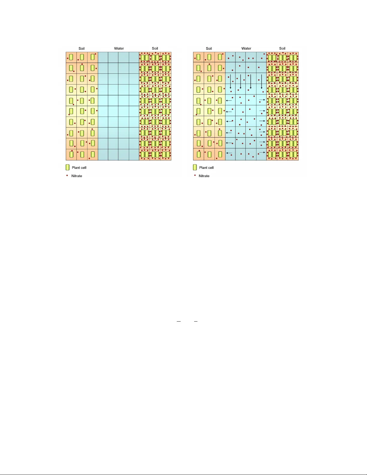
Proceedings of 5th W orkshop on Membrane Computing and Biologically Inspired Process Calculi (MeCBIC 2011) Pages 25–39, 2011. c  L. Bioglio, C. Calcagno, M. Coppo, F . Damiani, E. Sciacca, S. Spinella and A. T roina All the rights to the paper remain with the authors. A Spatial Calculus of Wrapped Compartments ∗ Li vio Bioglio 1 , Cristina Calcagno 1 , 2 , Mario Coppo 1 , Ferruccio Damiani 1 , Ev a Sciacca 1 , Salv atore Spinella 1 , Angelo T roina 1 1 Dipartimento di Informatica, Univ ersit ` a di T orino 2 Dipartimento di Biologia V egetale, Uni versit ` a di T orino The Calculus of Wrapped Compartments (CWC) is a recently proposed modelling language for the representation and simulation of biological systems beha viour . Although CWC has no explicit struc- ture modelling a spatial geometry , its compartment labelling feature can be exploited to model various examples of spatial interactions in a natural way . Howe ver , specifying large networks of compart- ments may require a long modelling phase. In this w ork we present a surface language for CWC that provides basic constructs for modelling spatial interactions. These constructs can be compiled away to obtain a standard CWC model, thus exploiting the existing CWC simulation tool. A case study concerning the modelling of Arbuscular Mychorrizal fungi gro wth is discussed. 1 Intr oduction Se veral complex biological phenomena include aspects in which space plays an essential role, key ex- amples are the gro wth of tissues and organisms, embryogenesis and morphogenesis processes or cell proliferation. This has encouraged, in recent years, the dev elopment of formal models for the description of biological systems in which spatial properties can be taken into account [9, 4, 19], as required by the emerging field of spatial systems biology [26] which aims at integrating the analysis of biological systems with spatial properties The Calculus of Wrapped Compartments (CWC) [12, 11, 10] is a calculus for the description of biochemical systems which is based on the notion of a compartment which represents, in some sense, the abstraction of a region with specific properties (characterized by a label , a wrap and a content ). Biochemical transformations are described via a set of stochastic reduction rules which characterize the behaviour of the represented system. In a recent work [7] we ha ve ha ve sho wn ho w CWC can be used to model spatial properties of bi- ological systems. The idea is to e xploit the notion of compartment to represent spatial regions (with a fixed, two-dimensional topology) in which the labels plays a key role in defining the spatial properties. In this framew ork, the mo vement and growth of system elements are described, via specific rules (in v olv- ing adjacent compartments) and the functionalities of biological components are affected by the spatial constraints gi ven by the sector in which the y interact with other elements. CWC allo ws to model sev eral spatial interactions in a very natural way . Ho wev er , when the complexity of simulation scenarios in- creases, the specification of large netw orks of compartments each one having its own peculiar behaviour and initial state may require a long and error prone modelling phase. In this paper we introduce a surf ace language for CWC that defines a framework in which the notion of space is included as an essential component of the system. The space is structured as a square grid, whose dimension must be declared as part of the system specification. The surface language provides ∗ This research is funded by the BioBITs Project ( Conver ging T echnologies 2007, area: Biotechnology-ICT), Regione Piemonte. basic constructs for modelling spatial interactions on the grid. These constructs can be compiled away to obtain a standard CWC model, thus exploiting the e xisting CWC simulation tool. A similar approach can be found in [19] where the topological structure of the components is ex- pressed via explicit links which require ad-hoc rules to represent mov ements of biological entities and a logic-oriented language to flexibly specify complex simulation scenarios is provided. In order to deal with larger biological systems, we are planning to extend the CWC to the spatial domain incrementally . At this early stage we ne glected to consider problems related to the increase of the spatial rules with the increasing dimension of the grid 1 . A partial solution to this problem is the use of appropriate data struc- tures to represent entities scattered on a grid. A further step in this direction should be that of allo wing the definition of dif ferent topological representations for spatial distributions of the biological entities, like in [7]. This requires, obviously , that also the surf ace language be enriched with primitiv es suitable to express different spatial topology and related concepts (like the notion of proximity of locations and that of movement in space). The right spatial topology could also help to minimize the number of spatial rules needed for modeling phenomena. A more ambitious goal will be that of providing a basis for com- putational geometry to our simulator , in order to identify spatially significant e vents for the simulation. This will requires ho wev er a much bigger implementation ef fort. Organisation of the Paper Section 2 recalls the CWC frame work. Section 3 presents the surface language needed to describe spatial terms and rules. Section 4 presents a case study concerning some spatial aspects in the modelling of Arb uscular Mychorrizal fungi. Section 5 concludes the paper by briefly discussing related w ork and possible directions for further work. The Appendix presents the software module implementing the surface language. 2 The Calculus of Wrapped Compartments The Calculus of Wrapped Compartments (CWC) (see [12, 10, 11]) is based on a nested structure of ambients delimited by membranes with specific proprieties. Biological entities like cells, bacteria and their interactions can be easily described in CWC. 2.1 T erm Syntax Let A be a set of atomic elements ( atoms for short), ranged over by a , b , ..., and L a set of compartment types represented as labels ranged over by ,  0 ,  1 , . . . A term of CWC is a multiset t of simple terms where a simple term is either an atom a or a compartment ( a c t 0 )  consisting of a wrap (represented by the multiset of atoms a ), a content (represented by the term t 0 ) and a type (represented by the label  ). As usual, the notation n ∗ t denotes n occurrences of the simple term t . W e denote an empty term with • . An example of CWC term is 2 ∗ a b ( c d c e f )  representing a multiset (multisets are denoted by listing the elements separated by a space) consisting of two occurrences of a , one occurrence of b (e.g. three molecules) and an  -type compartment ( c d c e f )  which, in turn, consists of a wrap (a membrane) with two atoms c and d (e.g. two proteins) on its surface, and containing the atoms e (e.g. a molecule) and f (e.g. a DN A strand). See Figure 1 for some other examples with a simple graphical representation. 1 note that in a 2D model the space-related rules grow according to the square of the grid dimension 26 (a) (b) (c) Figure 1: (a) represents ( a b c c • )  ; (b) represents ( a b c c ( d e c • )  0 )  ; (c) represents ( a b c c ( d e c • )  0 f g )  2.2 Rewriting Rules System transformations are defined by rewriting rules, defined by resorting to CWC terms that may contain v ariables. W e call pattern the l.h.s. component p of a rewrite rule and open term the r .h.s. component o of a re write rule, defined as multiset of simple patterns p and simple open terms o gi v en by the follo wing syntax: p :: = a   ( a x c p X )  o :: = a   ( q c o )    X q :: = a   x where a is a multiset of atoms, p is a pattern (a, possibly empty , multiset of simple patterns), x is a wrap variable (can be instantiated by a multiset of atoms), X is a content variable (can be instantiated by a CWC term), q is a multiset of atoms and wrap v ariables and o is an open term (a, possibly empty , multiset of simple open terms). Patterns are intended to match, via substitution of v ariables with ground terms (containing no variables), with compartments occurring as subterms of the term representing the whole system. Note that we force exactly one v ariable to occur in each compartment content and wrap of our patterns and simple patterns. This pre vents ambiguities in the instantiations needed to match a gi v en compartment. 2 A r e write rule is a triple ( , p , o ) , denoted by  : p 7− → o , where p and o are such that the v ariables occurring in o are a subset of the v ariables occurring in p . The application of a rule  : p 7− → o to a term t is performed in the follo wing w ay: 1) Find in t (if it e xists) a compartment of type  with content u and a substitution σ of v ariables by ground terms such that u = σ ( p X ) 3 and 2) Replace in t the subterm u with σ ( o X ) . W e write t 7− → t 0 if t 0 is obtained by applying a rewrite rule to t . The re write rule  : p 7− → o can be applied to any compartment of type  with p in its content (that will be rewritten with o ). For instance, the rewrite rule  : a b 7− → c means that in all compartments of type  an occurrence of a b can be replaced by c While the rule does not change the label  of the compartment where the rule is applied, it may change all the labels of the compartments occurring in its content. For instance, the rewrite rule  : ( a x c X )  1 7− → ( a x c X )  2 means that, if contained in a compartment of type  , all compartments of type  1 and containing an a in their wrap can change their type to  2 . For uniformity reasons we assume that the whole system is alw ays represented by a term consisting of a single compartment with distinguished label > and empty wrap, i.e., any system is represented by a 2 The linearity condition, in biological terms, corresponds to excluding that a transformation can depend on the presence of two (or more) identical (and generic) components in dif ferent compartments (see also [20]). 3 The implicit (distinguished) variable X matches with all the remaining part of the compartment content. 27 term of the shape ( • c t ) > , which will be also written as t , for simplicity . 2.3 Stochastic Simulation A stochastic simulation model for biological systems can be defined along the lines of the one presented by Gillespie in [14], which is, de facto , the standard way to model quantitativ e aspects of biological systems. The basic idea of Gillespie’ s algorithm is that a rate function is associated with each considered chemical reaction which is used as the parameter of an exponential distrib ution modelling the probability that he reaction takes place. In the standard approach this reaction rate is obtained by multiplying the kinetic constant of the reaction by the number of possible combinations of reactants that may occur in the region in which the reaction tak es place, thus modelling the law of mass action. For rules defining spatial mov ement the kinetic constant can be interpreted as the speed of the movement. In [12], the reaction rate is defined in a more general way by associating to each reduction rule a function which can also define rates based on dif ferent principles as, for instance, the Michaelis-Menten nonlinear kinetics. For simplicity , in this paper , we will follow the standard approach in defining reaction rates. Each reduction rule is then enriched by the kinetic constant k of the reaction that it represents (notation  : p k 7− → o ). For instance in ev aluating the application rate of the stochastic rewrite rule R =  : a b k 7− → c (written in the simplified form) to the term t = a a b b in a compartment of type  we must consider the number of the possible combinations of reactants of the form a b in t . Since each occurrence of a can react with each occurrence of b , this number is 4. So the application rate of R is k · 4. 2.4 The CWC simulator The CWC simulator [1] is a tool under de velopment at the Computer Science Department of the T urin Uni versity , based on Gillespie’ s direct method algorithm [14]. It treats CWC models with different rating semantics (law of mass action, Michaelis-Menten kinetics, Hill equation) and it can run independent stochastic simulations ov er CWC models, featuring deep parallel optimizations for multi-core platforms on the top of FastFlo w [2]. It also performs online analysis by a modular statistical framew ork. 3 A Surface Language In this section we embed CWC into a surface language able to express, in a synthetic form, both spatial (in a two-dimensional grid) and biochemical CWC transformations. The semantics of a surface language model is defined by translation into a standard CWC model. W e distinguish between two kind of compartments: 1. Standar d compartments (corresponding to the usual CWC compartments), used to represent enti- ties (like bacteria or cells) that can mo ve through space. 2. Spatial compartments, used to represent portions of space. Each spatial compartment defines a location in a two dimensional grid through a special atom, called coor dinate , that occurs on its wrap. A coordinate is denoted by row.column , where row and column are intergers. Spatial compartments hav e distinguished labels, called spatial labels , that can be used to provide a specific characterisation of a portion of space. 28 For simplicity we assume that the wraps of each spatial compartment contains only the coordinate. There- fore, spatial compartment dif ferentiations can be expressed only in terms of labels. 4 For e xample, the spatial compartment ( 1.2 c 2 ∗ b ) soil represents the cell of the grid located in the first row and the second column, and has type soil , the spatial compartment ( 2.3 c 3 ∗ b c ) water repre- sents a water -type spatial compartment in position 2.3 . In our grid we assume that molecules can float only through neighbor cells: all the rules of interaction between spatial compartments must obviously contain the indexes of their location. For example, the rule > : ( 1.2 x c a X ) water ( 2.2 y c Y ) soil k 7− → ( 1.2 x c X ) water ( 2.2 y c a Y ) soil mov es the molecule a from the water compartment in position 1.2 to the soil compartment in position 2.2 with a rate k representing in this case, the speed of the mov ement of a in do wnwards direction from a cell of water -type to a cell of soil -type. Let R and C denote the dimensions of our R × C grid defined by R rows and C columns. T o increase the e xpressivity of the language we define a fe w structures to denote portions (i.e. sets of cells) of the grid. With Θ we denote a set of coordinates of the grid and we use the notion r.c ∈ Θ when the coordinate r.c is contained in the set Θ . W e define rectangles by rect [ r.c , r’.c’ ] where r.c , r’.c’ represent the edges of the rectangle. W e project rows and columns of our grid with the constructions row [ i ] and col [ j ] respecti vely . Example 3.1 The set Θ = { 6 . 6 } ∪ rect [ 1 . 1 , 3 . 2 ] ∪ col [ 5 ] r epresents the set of coor dinates Θ = { 6 . 6 } ∪ { 1 . 1 , 2 . 1 , 3 . 1 , 1 . 2 , 2 . 2 , 3 . 2 } ∪ { i . 5 | ∀ i ∈ [ 1 , R ] } . Note that row [ i ] is just a shorthand for rect [ i.1 , i.C ]. Similarly for columns. W e use [*] as shorthand to indicate the whole grid (i.e. rect[1.1,R.C] ). W e also define four dir ection operators, N, W, S, E that applied to a range of cells shift them, respecti vely , up, left, do wn and right. F or instance E(1.1) = 1.2 . In the intuitiv e way , we also define the four diagonal mo vements (namely , NW , SW , NE , SE ). With ∆ we denote a set of directions and we use the special symbol  to denote the set containing all eight possible directions. W e con vene that when a coordinate, for effect of a shit, goes out of the range of the grid the corre- sponding point is eliminated from the set. 3.1 Surface T erms W e define the initial state of the system under analysis as a set of compartments modelling the two- dimensional grid containing the biological entities of interest. Let Θ denote a set of coordinates and  s a spatial label. W e use the notation: Θ ,  s  t to define a set of cells of the grid. Namely Θ ,  s  t denotes the top le vel CWC term: ( • c ( r 1 . c 1 c t )  s . . . ( r n . c n c t )  s ) > where r i . c j range ov er all elements of Θ . A spatial CWC term is thus defined by the set of grid cells cov ering the entire grid. 4 Allowing the wrap of spatial compartments to contain other atoms, thus providing an additional mean to express spatial compartment differentiations, should not pose particular technical problems (extend the rules of the surface language to deal with a general wrap content also for spatial compartments should be straightforward). 29 (a) Initial state (b) Spatial ev ents Figure 2: Graphical representations of the grid described in the Example 3 . 2. Example 3.2 The CWC term obtained by the thr ee grid cell constructions: rect [ 1 . 1 , 10 . 3 ] , soil  nit r ( rece p t ors c cyt o pl asm nucl eus ) Pl antCel l rect [ 1 . 4 , 10 . 7 ] , wat er  • rect [ 1 . 8 , 10 . 10 ] , soil  10 ∗ ni t r 2 ∗ ( r ece p t or s c cy t o pl asm nucl eus ) Pl antCel l builds a 10 × 10 grid composed by two portions of soil (the right-most one r eacher of nitrates and plant cells) divided by a river of water (see F igure 2(a)). 3.2 Surface Rewrite Rules W e consider rules for modelling three kind of ev ents. Non-Spatial Events: are described by standard CWC rules, i.e. by rules of the shape:  : p k 7− → o Non-spatial rules can be applied to any compartment of type  occurring in any portion of the grid and do not depend on a particular location. Example 3.3 A plant cell might perform its activity in any location of the grid. The following rules, describing some usual activities within a cell, might happen in any spatial compartment containing the plant cells under considerations: Pl antC el l : nucl eus k 1 7− → nucl eus mRN A Pl antC el l : mRN A cyt o pl asm k 2 7− → mRN A cyt o pl asm pr ot ein. Spatial Events: are described by rules that can be applied to specific spatial compartments. These rules allo w to change the spatial label of the considered compartment. Spatial e vents are described by rules of 30 the follo wing shape: Θ   s : p k 7− →  0 s : o Spatial rules can be applied only within the spatial compartments with coordinates contained in the set Θ and with the spatial label  s . The application of the rule may also change the label of the spatial compartments  s to  0 s . This rule is translated into the CWC set of rules: > : ( r i . c i x c p X )  s k 7− → ( r i . c i x c o X )  0 s ∀ r i . c i ∈ Θ . Note that spatial rules are analogous to non spatial ones. The only difference is the e xplicit indication of the set Θ which allows to write a single rule instead of a set of rule (one for each element of Θ ). Example 3.4 If we suppose that the river of water in the middle of the grid defined in Example 3.2 has a downwar d str eaming, we might consider the initial part of the river (framed by the first r ow rect[1.4,1.7] ) to be a sour ce of nitrates (as they ar e coming fr om a r e gion which is not modelled in the actual consider ed grid). The spatial rule: rect [ 1 . 4 , 1 . 7 ]  wa t er : • k 3 7− → wat er : ni t r models the arrival of nitrates at the first modeled portion of the river (in this case it does not c hange the label of the spatial compartment in volved by the rule). Spatial Movement Events: are described by rules considering the content of two adjacent spatial com- partments and are described by rules of the follo wing shape: Θ  ∆   s 1 ,  s 2 : p 1 , p 2 k 7− →  0 s 1 ,  0 s 2 : o 1 , o 2 This rule changes the content of tw o adjacent (according to the possible directions contained in ∆ ) spatial compartments and thus allo ws to define the mo vement of objects. The pattern matching is performed by checking the content of a spatial compartment of type  s 1 located in a portion of the grid defined by Θ and the content of the adjacent spatial compartment of type  s 2 . Such a rule could also change the labels of the spatial compartments. This rule is translated into the CWC set of rules: > : ( r i . c i x c p 1 X )  s 1 ( d ir ( r i . c i ) y c p 2 Y )  s 2 k 7− → ( r i . c i x c o 1 X )  0 s 1 ( d ir ( r i . c i ) y c o 2 Y )  0 s 2 for all r i . c i ∈ Θ and for all d ir ∈ ∆ . Example 3.5 W e assume that the flux of the river moves the nitrates in the water according to a down- war d dir ection in our grid and with a constant speed in any portion of the river with the following rule: rect [ 1 . 4 , 9 . 7 ]  { S }  wat er , wa t er : ni t r , • k 4 7− → wat er , wat er : • , nit r when nitrates r each the down-most r ow in our grid they just disappear (non moving e vent): rect [ 10 . 4 , 10 . 7 ]  wa t er : ni t r k 4 7− → wat er : • . Mor eover , nitrates str eaming in the river may be absorbed by the soil on the riverside with the rule: rect [ 1 . 4 , 10 . 7 ]  { W , E }  wat er , soil : nit r , • k 5 7− → wat er , soil : • , nit r . A graphical r epr esentation of these events is shown in F igur e 2(b). Other rules can be defined to move the nitrates within the soil etc. 4 Case Study: A Growth Model for AM Fungi In this section we illustrate a case study concerning the modelling of Arbuscular Mychorrizal fungi gro wth. 31 Figure 3: Extraradical mycelia of an arbuscular mycorrhizal fungus. 4.1 Biological Model The arbuscular mycorrhizal (AM) symbiosis is an example of association with high compatibility formed between fungi belonging to the Glomeromycota phylum and the roots of most land plants[15]. AM fungi are obligate symbionts, in the absence of a host plant, spores of AM fungi germinate and produce a limited amount of mycelium. The recognition between the two symbionts is driv en by the perception of diffusible signals and once reached the root surface the AM fungus enters in the root, overcomes the epidermal layer and it gro ws inter-and intracellularly all along the root in order to spread fungal structures. Once inside the inner layers of the cortical cells the dif ferentiation of specialized, highly branched intracellular hyphae called arb uscules occur . Arbuscules are considered the major site for nutrients exchange between the tw o org anisms. The fungus supply the host with essential nutrients such as phosphate, nitrate and other minerals from the soil. In return, AM fungi recei ve carbohydrates deri ved from photosynthesis in the host. Simultaneously to intraradical colonization, the fungus dev elops an extensi v e netw ork of hyphae which explores and exploits soil microhabitats for nutrient acquisition. AM fungi hav e different hyphal gro wth patterns, anastomosis and branching frequencies which result in the occupation of dif ferent niche in the soil and probably reflect a functional diversity [18] (see Figure 3). The mycelial netw ork that de velops outside the roots is considered as the most functionally di verse component of this symbiosis. Extraradical mycelia (ERM) not only provide extensi ve pathways for nutrient fluxes through the soil, but also hav e strong influences upon biogeochemical cycling and agro-ecosystem functioning [22]. The mechanisms by which fungal networks extend and function remain poorly characterized. The functioning of ERM presumably relies on the existence of a complex regulation of fungal gene expression with reg ard 32 to nutrient sensing and acquisition. The fungal life c ycle is then completed by the formation, from the external mycelium, of a ne w generation of spores able to survi ve under unf a vourable conditions. In v estigations on carbon (C) metabolism in AM fungi hav e proved useful to offer some explanation for their obligate biotrophism. As mentioned above, an AM fungus relies almost entirely on the host plant for its carbon supply . Intraradical fungal structures (presumably the arb uscules) are known to take up photosynthetically fix ed plant C as hexoses. Unfortunately , no fungal he xose transporter -coding gene has been characterized yet in AM fungi. In order to quantify the contribution of arbuscular mycorrhizal (AM) fungi to plant nutrition, the de velopment and e xtent of the external fung al mycelium and its nutrient uptake capacity are of particular importance. Shnepf and collegues [25] developed and analysed a model of the extraradical growth of AM fungi associated with plant roots considering the gro wth of fungal hyphae from a cylindrical root in radial polar coordinates. Measurements of fungal growth can only be made in the presence of plant. Due to this practical dif ficulty experimental data for calibrating the spatial and temporal explicit models are scarce. Jakobsen and collegues [16] presented measurements of hyphal length densities of three AM fungi: Scutellospora calospora (Nicol.& Gerd.) W alker & Sanders; Glomus sp. associated with clover ( T rifolium subterra- neum L.);these data appeared suitable for comparison with modelled hyphal length densities. The model in [25] describes, by means of a system of Partial Dif ferential Equations (PDE), the de- velopment and distrib ution of the fungal mycelium in soil in terms of the creation and death of hyphae, tip-tip and tip-hypha anastomosis, and the nature of the root-fungus interface. It is calibrated and cor - roborated using published experimental data for hyphal length densities at dif ferent distances away from root surfaces. A good agreement between measured and simulated v alues was found for the three fungal species with dif ferent morphologies associated with T rifolium subterr aneum L. The model and findings are expected to contribute to the quantification of the role of AM fungi in plant mineral nutrition and the interpretation of dif ferent foraging strategies among fungal species. 4.2 Surface CWC Model In this Section we describe ho w to model the growth of arb uscular mycorrhyzal fungi using the surface spatial CWC. W e model the gro wth of AM fungal hyphae in a soil en vironment partitioned into 13 dif- ferent layers (spatial compartments with label soil ) to account for the distance in centimetres between the plant root and the fungal hyphae where the soil layer at the interface with the plant root is at posi- tion 1 . 1. W e describe the mycelium by two atoms: the h yphae (atom H y p ) related to the length densities (number of hyphae in a gi ven compartment) and the hyphal tips (atom T i p ). The plant root (atom Root ) is contained in the soil compartment at position 1 . 1. The tips and hyphae at the root-fungus interface proliferate according to the following spatial e vents: { 1 . 1 }  soil : Root ˜ a 7− → soil : Root H y p { 1 . 1 }  soil : Root a 7− → soil : Root T i p where ˜ a and a is the root proliferation factor for the hyphae and tips respecti v ely . Hyphal tips are important, because growth occurs due to the elongation of the region just behind the tips. Therefore, the spatial mov ement ev ent describing the hyphal segment created during a tip shift to a nearby compartment is: 33 [ ∗ ]  { E , W }  soil , soil : T i p , • v 7− → soil , soil : H y p , T i p where v is the rate of tip mov ement. The hyphal length is related to tips mov ement, i.e. an hyphal trail is left behind as tips mov e through the compartments. W e consider hyphal death to be linearly proportional to the hyphal density , so that the rule describing this spatial event is: [ ∗ ]  soil : H y p d H 7− → soil : • where d H is the rate of hyphal death. Mycorrhizal fungi are known to branch mainly apically where one tip splits into two. In the simplest case, branching and tip death are linearly proportional to the e xisting tips in that location modelled with the follo wing spatial ev ents: [ ∗ ]  soil : T i p b T 7− → soil : 2 ∗ T i p [ ∗ ]  soil : T i p d T 7− → soil : • where b T is the tip branching rate and d T is the tip death rate. Alternati vely , if we assume that branching decreases with increasing tip density and ceases at a gi ven maximal tip density , we employ the spatial e vent: [ ∗ ]  soil : 2 ∗ T i p c T 7− → soil : • where c T = b T T max . From a biological point of view , this beha viour take into account the v olume saturation when the tip density achie ves the maximal number of tips T max . The fusion of two hyphal tips or a tip with a hypha can create interconnected networks by means of anastomosis: [ ∗ ]  soil : 2 ∗ T i p a 1 7− → soil : T i p [ ∗ ]  soil : T i p H y p a 2 7− → soil : T i p where a 1 and a 2 are the tip-tip and tip-hypha anastomosis rate constants, respecti vely . The initial state of the system is gi ven by the follo wing grid cell definition: { 1 . 1 } , soil  Root T 0 ∗ T i p H 0 ∗ H y p rect [ 1 . 2 , 1 . 13 ] , soil  • where T 0 and H 0 are the initial number of tips and hyphae respectiv ely at the interface with the plant root. 4.3 Results W e run 60 simulations on the model for the fungal species Scutellospora calospora and Glomus sp. Figure 4 sho w the mean v alues of hyphae (atoms H y p ) of the resulting stochastic simulations in function of the elapsed time in days and of the distance from the root surface. The rate parameters of the model are taken from [25]. The results for S. calospora are in accordance with the linear PDE model of [25] which is charac- terized by linear branching with a relatively small net branching rate and both kinds of anastomosis are 34 0 2 4 6 8 10 12 0 5 10 15 20 25 30 35 40 45 50 0 20 40 60 80 100 120 number of hyphae distance from root (cm) time (days) number of hyphae 0 20 40 60 80 100 120 0 2 4 6 8 10 12 0 5 10 15 20 25 30 35 40 45 50 0 5 10 15 20 25 30 35 number of hyphae distance from root (cm) time (days) number of hyphae 0 5 10 15 20 25 30 35 Figure 4: Mean v alues of 60 stochastic simulations of hyphal growth (atoms H y p ) results for S. calospora and Glomus sp. fungi. negligible when compared with the other species. This model imply that the fungus is mainly gro wing and allocating resources for getting a wider catchment area rather than local expoloitation of mineral resources via hyphal branching. The model for Glomus sp. considers the effect of nonlinear branching due to the competition be- tween tips for space. The results obtained for Glomus sp. are in accordance with the non–linear PDE model of [25] which imply that local exploitation for resources via hyphal branching is important for this fungus as long as the hyphal tip density is small. Reaching near the maximum tip density , branching decreases. Symbioses between a given host plant and different AM fungi have been shown to dif fer functionally [23]. 5 Conclusions and Related W orks For the well-mixed chemical systems (e ven divided into nested compartments) often found in cellular biology , interaction and distribution analysis are sufficient to study the system’ s behaviour . Howe ver , there are many other situations, like in cell growth and de velopmental biology where dynamic spatial arrangements of cells determines fundamental functionalities, where a spatial analysis becomes essential. Thus, a realistic modelling of biological processes requires space to be taken into account [17]. This has brought to the extension of many formalisms dev eloped for the analysis of biological sys- tems with (e ven continuous) spatial features. In [9], Cardelli and Gardner develop a calculus of processes located in a three-dimensional geometric space. The calculus, introduces a single new geometric construct, called frame shift , which applies a three-dimensional space transformation to an e volving process. In such a work, standard notions of process equi valence gi ve rise to geometric in v ariants. In [5], a varia nt of P-systems embodying concepts of space and position inside a membrane is pre- sented. The objects inside a membrane are associated with a specific position. Rules can alter the position of the objects. The authors also define exclusive objects (only one exclusi ve object can be contained in- side a membrane). In [3], an spatial extension of CLS is given in a 2D/3D space. The spatial terms of the calculus may move autonomously during the passage of time, and may interact when the constraints on their positions are satisfied. The authors consider a hard-spher e based notion of space: two objects, represented as spheres, cannot occupy the same space, thus conflicts may arise by mo ving objects. Such 35 conflicts are resolved by specific algorithms considering the forces in volv ed and appropriate pushing among the objects. BioShape [6] is a spatial, particle-based and multi-scale 3D simulator . It treats biological entities of dif ferent size as geometric 3D shapes . A shape is either basic (polyhedron, sphere, cone or cylinder) or composed (aggregation of shapes glued on common surfaces of contact). Every element inv olv ed in the simulation is a 3D process and has associated its physical motion law . Adding too many features to the model (e.g., coordinates, position, extension, motion direction and speed, rotation, collision and ov erlap detection, communication range, etc.) could heavily rise the com- plexity of the analysis. T o ov ercome this risk, a detailed study of the possible subsets of these features, chosen to meet the requirements of particular classes of biological phenomena, might be considered. In this paper we pursued this direction by extending CWC with a surface language providing a frame work for incorporating basic spatial features (namely , coordinates, position and mov ement). In fu- ture work we plan to extend the surf ace language to deal with three dimensional spaces and to in vestigate the possibility to incorporate other spatial features to the CWC simulation frame work. Notably , the framew ork presented in this paper could also be applied to other calculi which are able to express compartmentalisation (see, e.g., BioAmbients [24], Brane Calculi [8], Beta-Binders [13], etc.). Refer ences [1] M. Aldinucci, M. Coppo, F . Damiani, M. Drocco, E. Giov annetti, E. Grassi, E. Sciacca, S. Spinella & A. T roina (2010): CWC Simulator . Dipartimento di Informatica, Universit ` a di T orino. http:// cwcsimulator.sourceforge.net/ . [2] M. Aldinucci & M. T orquati (2009): F astFlow website . FastFlo w . http://mc- fastflow.sourceforge. net/ . [3] R. Barbuti, A. Maggiolo-Schettini, P . Milazzo & G. Pardini (2009): Spatial Calculus of Looping Sequences . Electr . Notes Theor . Comput. Sci. 229(1), pp. 21–39. A vailable at http://dx.doi.org/10.1016/j. entcs.2009.02.003 . [4] R. Barbuti, A. Maggiolo-Schettini, P . Milazzo & G. Pardini (2011): Spatial Calculus of Looping Sequences . Theoretical Computer Science . [5] R. Barb uti, A. Maggiolo-Schettini, P . Milazzo, G. Pardini & L. T esei (2011): Spatial P systems . Natural Computing 10(1), pp. 3–16. A v ailable at http://dx.doi.org/10.1007/s11047- 010- 9187- z . [6] F . Buti, D. Cacciagrano, F . Corradini, E. Merelli & L. T esei (2010): BioShape: A Spatial Shape-based Scale- independent Simulation En vir onment for Biological Systems . Procedia CS 1(1), pp. 827–835. A vailable at http://dx.doi.org/10.1016/j.procs.2010.04.090 . [7] C. Calcagno, M. Coppo, F . Damiani, M. Drocco, E. Sciacca, S. Spinella & A. T roina (T o Appear): Modelling Spatial Interactions in the AM Symbiosis using CWC . In: CompMod 2011 . [8] L. Cardelli (2004): Brane Calculi . In: Proc. of CMSB’04 , LNCS 3082, Springer , pp. 257–278. [9] L. Cardelli & P . Gardner (2010): Pr ocesses in Space . In: Proc. of the 6th international conference on Computability in Europe , CiE’10, Springer-V erlag, pp. 78–87. [10] M. Coppo, F . Damiani, M. Drocco, E. Grassi, M. Guether & A. T roina (2011): Modelling Ammonium T rans- porters in Arbuscular Mycorrhiza Symbiosis . Transactions on Computational Systems Biology XIII, pp. 85–109. [11] M. Coppo, F . Damiani, M. Drocco, E. Grassi, E. Sciacca, S. Spinella & A. T roina (2010): Hybrid Calculus of Wrapped Compartments . In: Proceedings Compendium of the Fourth W orkshop on Membrane Computing and Biologically Inspired Process Calculi (MeCBIC’10) , 40, EPTCS, pp. 103–121. 36 [12] M. Coppo, Damiani. F ., M. Drocco, Grassi. E. & A. T roina (2010): Stochastic Calculus of Wrapped Com- partments . In: 8th W orkshop on Quantitativ e Aspects of Programming Languages (QAPL ’10) , 28, EPTCS, pp. 82–98. [13] P . Deg ano, D. Prandi, C. Priami & P . Quaglia (2006): Beta-binders for Biological Quantitative Experiments . Electr . Notes Theor . Comput. Sci. 164(3), pp. 101–117. A vailable at http://dx.doi.org/10.1016/j. entcs.2006.07.014 . [14] D. Gillespie (1977): Exact Stochastic Simulation of Coupled Chemical Reactions . J. Phys. Chem. 81, pp. 2340–2361. [15] M.J. Harrison (2005): Signaling in the Arbuscular Mycorrhizal Symbiosis . Annu. Re v . Microbiol. 59, pp. 19–42. [16] I. Jakobsen, LK Abbott & AD Robson (1992): External Hyphae of V esicular-arb uscular Mycorrhizal Fungi Associated with T rifolium Subterraneum L. 1. Spr ead of Hyphae and Phosphorus Inflow into Roots . Ne w Phytologist 120(3), pp. 371–379. [17] B. Kholodenko (2006): Cell-signalling Dynamics in T ime and Space . Nature Revie ws Molecular Cell Biol- ogy 7, pp. 165–176. [18] H. Maherali & J.N. Klironomos (2007): Influence of Phylogeny on Fungal Community Assembly and Ecosys- tem Functioning . Science 316(5832), p. 1746. [19] S. Montagna & M. V iroli (2010): A F rame work for Modelling and Simulating Networks of Cells . Electr . Notes Theor . Comput. Sci. 268, pp. 115–129. A vailable at http://dx.doi.org/10.1016/j.entcs.2010.12. 009 . [20] N. Oury & G. Plotkin (2011): Multi-Level Modelling via Stochastic Multi-Level Multiset Re writing . Draft submitted to MSCS. [21] T . Parr et al.: ANTLR website . http://www.antlr.org/ . [22] S. Purin & M.C. Rillig (2008): P arasitism of Arb uscular Mycorrhizal Fungi: Reviewing the Evidence . FEMS Microbiology Letters 279(1), pp. 8–14. [23] S. Ravnsko v & I. Jakobsen (1995): Functional Compatibility in Arbuscular Mycorrhizas Measur ed as Hyphal P transport to the Plant . Ne w Phytologist 129(4), pp. 611–618. [24] A. Rege v , E. M. Panina, W . Silv erman, L. Cardelli & E. Y . Shapiro (2004): BioAmbients: An Abstraction for Biological Compartments . Theor . Comput. Sci. 325(1), pp. 141–167. [25] A. Schnepf, T . Roose & P . Schweiger (2008): Gr owth Model for Arbuscular Mycorrhizal Fungi . Journal of The Royal Society Interface 5(24), p. 773. [26] A. Spicher , O. Michel & J.-L. Giavitto (2011): Interaction-Based Simulations for Inte grative Spatial Systems Biology . In: Understanding the Dynamics of Biological Systems , Springer New Y ork, pp. 195–231. A ppendix: Implementation of the Surface Language This Section presents a software module implementing the translation of a surf ace language model into the corresponding standard CWC model that can be executed by the CWC simulator (cf. Sec. 2.4). The module is written in Jav a by means of the ANTLR parser generator [21]. The input syntax of the software is defined as follo wing. P atterns, T erms and Open T erms: pattern, terms and open terms follo w the syntax of CWC. In the definition of a compartment, its label is written in braces, as the first element in the round brackets. The symbol c is translated into | , and the empty sequence • into \ e . If a pattern, term or open term is repeated se veral times, we write the number of repetitions before it. Grid Coordinates: the row and the column of a grid coordinate are divided by a comma. All the con- structions of the surface language are implemented. The components of a set of coordinates are di vided by a blank space. 37 Dir ections: for the directions we use the same keyw ords of the surface language, plus the special iden- tifiers + , x , * to identify all the orthogonal directions ( N , S , W , E ), all the diagonal directions ( NW , SW , NE , SE ) and all the directions, respecti vely . Model Name: the name of the model is defined following the syntax model st r ing ; where s t r ing is the name of the model. Grid Dimensions: the dimensions of the grid are expressed with the syntax grid r , c ; where r and c are the number of rows and columns of the grid, respecti vely . Grid Cell Construction: the notation of a grid cell Θ ,  s  t is translated into the code line cell < Θ > {  s } t ; the module writes as many CWC compartments as the number of coordinates in Θ : each of these copies has the same label  s and the same content t , but a dif ferent coordinate in the wrap. Non Spatial Events: the notation of a non spatial event  : p k 7− → o is translated into the code line nse {  } p [ k ] o ; the module translates this line in a unique CWC rule. Spatial Events: the notation of a spatial event Θ   s : p k 7− →  0 s : o is translated into the code line se < Θ > {  s } p [ k ] {  0 s } o ; As shortcuts, the absence of < Θ > indicates the whole grid, and the absence of {  0 s } indicates that the label of the spatial compartment does not change. The module writes a CWC rule for each coordinate in Θ : a rule differs from the others only in the coordinate written in its wrap. Spatial Movement Events: the notation of a spatial movement e vent Θ  ∆   s 1 ,  s 2 : p 1 , p 2 k 7− →  0 s 1 ,  0 s 2 : o 1 , o 2 is translated into the code line sme < Θ > [ ∆ ] {  s 1 } p 1 {  s 2 } p 2 [ k ] {  0 s 1 } o 1 {  0 s 2 } o 2 ; As shortcuts, the absence of < Θ > indicates the whole grid, and the absence of {  0 s 1 } or {  0 s 2 } indicates that the label of the spatial compartment does not change. In case of absence of {  0 s 2 } , an underscore is used to separate o 1 and o 2 . For each coordinate in Θ , the module writes as many CWC rules as the number of directions in ∆ ; in case of a coordinate on the edge of the grid, the module writes a CWC rule for a direction only if this one identifies an adjacent spatial compartment on the grid. The number of CWC rules is therefore less or equal to | Θ | × | ∆ | . Monitors: a monitor permits to e xpose what pattern we need to monitor: at the end of simulation, all the states of this pattern are written in a log file. The syntax to design a monitor is the following: monitor st r ing < Θ > {  s } p ; where s t r ing is a string describing the monitor and p is the pattern, contained into a spatial compartment labelled by  s and the coordinates Θ , to monitor . As shortcut, the absence of < Θ > indicates the av erage of the monitors in the whole grid, and the absence of {  s } indicates to write a monitor for each label defined in the model. The module writes a monitor for each coordinate in Θ ; in case of the absence of {  s } , the module writes a monitor for each combination of coordinates in Θ and spatial labels defined in the model. The construction of a model follo ws the order used to describe the translator syntax: first the model name and the grid dimensions, then the rules of the model. After the rules, we define the grid cell, and finally the monitors. Listings 1 and 2 sho w the input file for the CWC Surface Language software to model the S. calospora and Glomus sp. fungi growth. 38 Listing 1: Input file for the Surface Language parser to model the S. calospora fungus gro wth m o d e l " A M F u n g i G r o w t h M o d e l S . C a l o s p o r a " ; g r i d 1 , 1 3 ; / / T i p s a n d h y p h a e p r o l i f e r a t i o n a t t h e r o o t - f u n g u s i n t e r f a c e s e < 0 , 0 > { g r i d } R o o t [ 2 . 5 2 ] R o o t T i p ; s e < 0 , 0 > { g r i d } R o o t [ 3 . 5 ] R o o t H y p ; / / T i p s b r a n c h i n g a n d d e a t h s e { g r i d } T i p [ 0 . 0 2 ] 2 T i p ; s e { g r i d } T i p [ 0 . 0 0 5 2 ] \ e ; / / H y p h a e d e a t h s e { g r i d } H y p [ 0 . 1 8 ] \ e ; / / H y p h a l c r e a t i o n d u r i n g a t i p s h i f t t o a n e a r b y c o m p a r t m e n t s m e [ E W ] { g r i d } T i p { g r i d } \ e [ 0 . 1 2 5 ] H y p _ T i p ; / / I n i t i a l s t a t e c e l l < 0 , 0 > { g r i d } R o o t 9 7 T i p 1 1 5 H y p ; c e l l < r e c t [ 0 , 1 0 , 1 2 ] > { g r i d } \ e ; m o n i t o r " H y p " < r e c t [ 0 , 0 0 , 1 2 ] > { g r i d } H y p ; Listing 2: Input file for the Surface Language parser to model the Glomus sp. fungus gro wth m o d e l " A M F u n g i G r o w t h M o d e l G l o m u s s p . " ; g r i d 1 , 1 3 ; / / T i p s a n d h y p h a e p r o l i f e r a t i o n a t t h e r o o t - f u n g u s i n t e r f a c e s e < 0 , 0 > { g r i d } R o o t [ 2 . 2 4 ] R o o t T i p ; s e < 0 , 0 > { g r i d } R o o t [ 1 . 0 4 ] R o o t H y p ; / / T i p s b r a n c h i n g a n d d e a t h s e { g r i d } T i p [ 1 . 9 1 ] 2 T i p ; s e { g r i d } T i p [ 0 . 1 5 ] \ e ; / / T i p s s a t u r a t i o n s e { g r i d } 2 T i p [ 0 . 1 5 ] \ e ; / / H y p h a e d e a t h s e { g r i d } H y p [ 0 . 2 8 ] \ e ; / / H y p h a l c r e a t i o n d u r i n g a t i p s h i f t t o a n e a r b y c o m p a r t m e n t s m e [ E W ] { g r i d } T i p { g r i d } \ e [ 0 . 0 6 5 ] H y p _ T i p ; / / I n i t i a l s t a t e c e l l < 0 , 0 > { g r i d } R o o t 8 4 T i p 3 5 H y p ; c e l l < r e c t [ 0 , 1 0 , 1 2 ] > { g r i d } \ e ; m o n i t o r " H y p " < r e c t [ 0 , 0 0 , 1 2 ] > { g r i d } H y p ; 39