Sparse Signal Recovery with Temporally Correlated Source Vectors Using Sparse Bayesian Learning

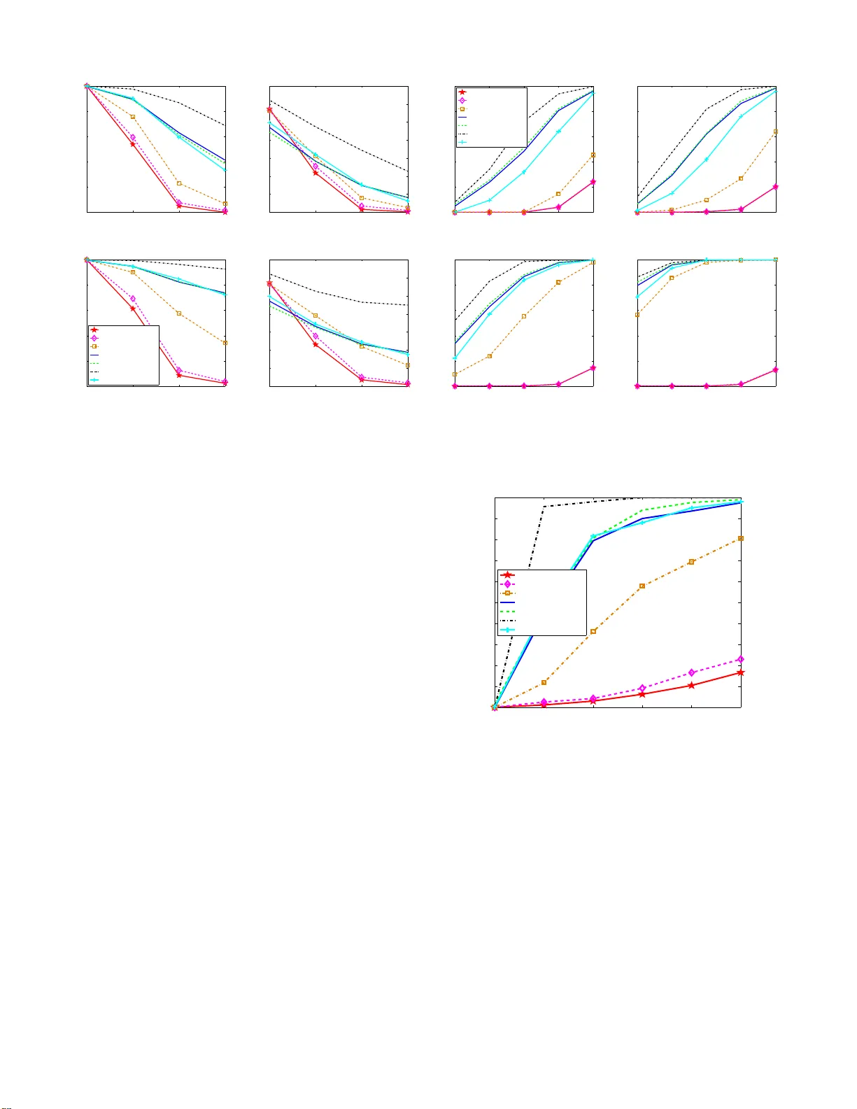
TO APPEAR IN IEE E JOURNAL OF SELECTED TOPICS IN SIGN AL PROCESSING, VOL.5, NO.5, 2011 1 Sparse Signal Reco v er y with T emporally Correlate d Source V ectors Using Sparse Bayesian Learning Zhilin Zhang, Student Member , IEEE and Bha skar D. Rao, F ellow , IEEE Abstract — W e address the sparse signal recov ery problem in the context of mul tiple measurem ent vectors (MM V) when elements in each nonzero row o f the solution matrix are tem- porally correla ted. Existing algorithms d o not consider such temporal correlation and thus their p erf ormance degrades si g- niﬁcantly with the correlation. In this work, we propose a block sparse Bayesian learning framew ork whi ch models the temporal correlation. W e derive two sparse Bayesian learning (SBL) algorithms, which ha ve superior re cov ery perform ance compared to existing algorithms, esp ecially in the presence of high temp oral correlation. Fu rthermore , our algorithms are better at handling highly underdetermined problems a nd require less row-sparsity on the solution matrix. W e also pr ovide analysis of the global and local minima of their co st function, and show that the SBL cost function has the very desirable property that the global m inimum is at the sp arsest solution to th e MMV problem. Extensive experiments also provide some interesting results that motivate future theoretical research on th e M MV model. Index T erms — Sparse Signal Recovery , Compressed Sensing, Sparse Bayesia n Learning (SBL), Multiple Measurement V ectors (MMV), T emporal Correlation I . I N T RO D U C T I O N Sparse signal recovery , or compressed sensing, is an emerg- ing ﬁeld in sig nal processing [1] –[4]. The basic mathematical model is y = Φx + v , (1) where Φ ∈ R N × M ( N ≪ M ) is a known dictionary matrix , and any N co lumns of Φ are linearly independen t (i.e. satisﬁ es the Uniqu e Represen tation Pr operty (URP) condition [5] ), y ∈ R N × 1 is a n a vailable measurem ent vector , and v is an u nknown n oise vector . The task is to e stimate the so urce vector x . T o e nsure a u nique g lobal solution, the number of n onzero entries in x has to be less th an a thresho ld [5 ], [6]. This single measuremen t vector (SMV) model (1) has a wide ran ge o f app lications, su ch as elec troenceph alograph y (EEG)/Magn etoenceph alography (MEG) source localization [7], d irection-o f-arriv al (DOA) estimation [8 ], r adar detec tion [9], and magn etic resonan ce imagin g (MRI) [10] . Motiv ated b y m any applications such as E EG/MEG source localization and DO A estimation, wh ere a sequen ce of mea- surement vectors are a vailable, the basic m odel (1) has been extended to the multiple measuremen t vector (MMV) mo del in [11] , [12] , given by Y = ΦX + V , (2) Z.Zhang and B.D.Rao are with the Depart ment of Elec trical and Computer Engineeri ng, Univ ersity of California at San Diego, La Jolla, CA 92093- 0407, USA. Em ail: { z4zhang ,brao } @ucsd.edu . T he work was supported by NSF grant CCF-0830612 . where Y , [ Y · 1 , · · · , Y · L ] ∈ R N × L is an av ailable mea- surement m atrix c onsisting of L me asurement vector s, X , [ X · 1 , · · · , X · L ] ∈ R M × L is an unknown source matrix (or called a solution matr ix) with each row representing a possible source 1 , and V is an unknown n oise matrix. A ke y assumption in the MMV mo del is that the supp ort ( i.e. indexes of nonzero entries) of ev ery column in X is iden tical (referred as th e common sparsity assumption in liter ature [12]) . In addition, similar to the constraint in the SMV model, the number of nonzer o rows in X has to b e below a thr eshold to e nsure a unique and glob al solution [12 ]. This leads to the fact that X has a small numb er of non zero rows. It has b een shown that com pared to the SMV case, th e successful recovery rate can be greatly improved u sing multi- ple measure ment vecto rs [ 12]–[1 5]. For example, Cotter and Rao [1 2] showed that by taking advantage of the MMV formu lation, on e can relax the up per bound in the u niqueness condition fo r the solu tion. T ang , Eldar a nd their colleagues [14], [16] showed that und er certain mild assumptio ns the recovery rate increases exponen tially with the number of measuremen t vectors L . Jin and Rao [ 15], [17] analyzed the beneﬁts of in creasing L by r elating th e MMV mo del to the capacity regions of MIMO comm unication chan nels. All these theoretical r esults r ev eal the advantages of the MMV model and suppor t increasing L for be tter rec overy performan ce. Howe ver, under the comm on sparsity assumption we cannot obtain many measureme nt vectors in practical application s. The main reason is that the sp arsity proﬁle of prac tical signals is (slowly) time-varying, so the commo n spar sity assump tion is valid for only a small L in the MMV m odel. For e xample, in EEG/MEG source localization there is con siderable evidence [18] that a giv en pattern of dipole-sou rce distrib utions 2 may only exist for 1 0-20 ms. Since the EEG/MEG sampling frequen cy is gene rally 25 0 Hz, a dipo le-source p attern m ay only exist th rough 5 snapshots (i.e. in the MMV model L = 5 ). In DOA estimation [1 9], directions of targets 3 are continuo usly chang ing, and thus the source vectors that satisfy the commo n spar sity a ssumption are f ew . Of course, one can increase the measurement vector n umber at the cost of increasing the sourc e number, but a larger source number can result in degraded rec overy performan ce. Thanks to numerou s algorithm s f or th e basic SMV mo del, 1 Here for con venie nce we call each ro w in X a source. The term is often used in applica tion-orie nted literature . Throughout the work, the i -th source is denot ed by X i · . 2 In this applicati on the set of indexe s of nonzero rows in X is called a patte rn of dipole-source distributio n. 3 In this applicatio n the inde x of a nonzero ro w in X indi cates a dire ction. TO APPEAR IN IEE E JOURNAL OF SELECTED TOPICS IN SIGN AL PROCESSING, VOL.5, NO.5, 2011 2 most MMV algorithms 4 are obtained by straightforward extension of the SMV algorithms; fo r example, calculating the ℓ 2 norm of each row of X , f orming a vector , and then imposing the sparsity constraint on the vector . These algo - rithms can b e roughly d i vided in to g reedy alg orithms [2 0], [21], algo rithms based on mixed nor m optimization [2 2]– [24], iterative reweighted algo rithms [12 ], [25 ], and Bayesian algorithm s [26], [27]. Among the MM V algorithm s, Bayesian algorithms hav e re- ceiv ed much attention recently s ince they generally achie ve the best recovery performa nce. Sp arse Bayesian lear ning (SBL) is o ne impor tant family of Bayesian algo rithms. It was ﬁrst propo sed by Tipping [28], [2 9], a nd then was gr eatly enriched and extended by many researcher s [25] –[27] , [30]–[3 6]. For example, Wipf and Rao ﬁr st in troduced SBL to sparse sig nal recovery [3 0] for the SMV mod el, and late r extended it to the MMV model, deriving the MSBL algorithm [26]. One attraction o f SBL/MSBL is th at, different from the popular ℓ 1 minimization based algor ithms [37], [38], whose g lobal minimum is ge nerally not the sp arsest solution [ 30], [39], the global min ima of SBL/MSBL are a lw ays the sparsest one. In addition, SBL/MSBL hav e mu ch fewer local minima than some classic algor ithms, such as the FOCUSS family [5], [12]. Motiv ated by application s wh ere signa ls and other types of data of ten contain so me kind of stru ctures, many algo- rithms have be en p roposed [13], [40 ]–[42 ], which exploit special stru ctures in the sour ce matrix X . Howe ver, mo st of these w orks fo cus on e xploiting spatial stru ctures (i.e. the dependency relationsh ip among different so urces) and completely ignore tem poral structu res. Besides, for tra ctability purpo ses, almost all the existing MMV algo rithms (an d theo- retical an alysis) assume that the sources are indepen dent and identically d istributed (i.i.d.) pr ocesses. This contradicts th e real-world scenarios, since a pr actical source o ften has rich temporal stru ctures. For example, the wav eform smo othness of biomedica l signals h as been explo ited in signal processing for several decad es. Besides, due to hig h sampling frequ ency , amplitudes of succe ssi ve samp lings of a sou rce are stron gly correlated. Recen tly , Zdun ek and Cichocki [4 3] pro posed the SOB-MFOCUSS alg orithm, wh ich exploits the waveform smoothne ss via a pre- deﬁned smoo thness matrix. Howe ver, the d esign of th e smoo thness m atrix is completely subjective and n ot data-adap ti ve. In fact, in th e task of sparse signal recovery , learnin g temporal structu res of a source is a difﬁcult problem . Generally , such structures are lear ned via a train ing dataset (which often contains sufﬁcient data withou t no ise for robust statistical infe rence) [4 4], [45]. Although effecti ve f or some sp eciﬁc signals, this meth od is limited. Having n oticed that the temporal struc tures strongly affect the perfor mance of existing algorithms, in [31] we derived t he AR-SBL algo rithm, which m odels each sou rce as a ﬁrst-order autoregre ssi ve (AR) process and learns AR coef ﬁcients from the data per se. Although the algo rithm has superior per forman ce compar ed to MM V algorithm s in the p resence of tempora l co rrelation, it is slow , which limits its app lications. As suc h, ther e is a 4 For con venien ce, algorithms for the MMV model are called MMV algorit hms; algo rithms for the SMV model are called SMV algorit hms. need for efﬁcient algorithm s that can d eal mo re effectively with tem poral correlatio n. In this work, we present a block sparse Bayesian learn ing (bSBL) fra mew ork, which tran sforms the MMV m odel (2) to a SMV mod el. This fr amew ork allows us to easily mod el the temporal co rrelation of sources. Based on it, we derive an algorithm , called T -SBL, which is very effectiv e but is slow due to its oper ation in a higher dimensional p arameter spac e resulting fro m the MMV -to-SMV transform ation. Th us, we make some appr oximations and derive a fast version , called T - MSBL, which operates in the original parameter space. Si milar to T -SBL, T -MSBL is also effective but has much lower c om- putational complexity . In terestingly , when compared to MSB L, the o nly change of T -MSBL is the replacem ent of k X i · k 2 2 with the M ahalanobis distance measure, i.e. X i · B − 1 X T i · , wh ere B is a positive deﬁnite m atrix e stimated from data and can b e partially interpreted a s a c ov ariance matr ix. W e analyze the global minimu m and the loca l minima of th e two algorith ms’ cost fu nction. On e of the key results is that in the noiseless case th e global minimum is at the sparsest solution. Extensive experiments not o nly show the sup eriority of th e prop osed algorithm s, but also provide some inter esting ( e ven co unter- intuitive) phen omena that may moti vate futu re theoretical study . The rest of the work is o rganized as follows. In Section II we present the bSBL fra mew o rk. In Section III we der i ve the T -SBL algorith m. Its fast version, the T -MSBL algorithm , is d eriv ed in Sectio n IV. Section V provides th eoretical analysis on the algorith ms. Expe rimental results are presented in Section VI. Finally , discussion s and co nclusions are dr awn in th e last two sectio ns. W e introd uce the n otations u sed in th is paper: • k x k 1 , k x k 2 , k A k F denote th e ℓ 1 norm of th e vector x , the ℓ 2 norm of x , and the Frobenius n orm of the ma trix A , respectiv ely . k A k 0 and k x k 0 denote the number of nonzer o rows in the m atrix A and th e num ber of n onzero elements in th e vector x , resp ecti vely; • Bold sy mbols a re reserved for vectors and matrices. Particularly , I L denotes the identity m atrix with size L × L . When the dimensio n is evident from the co ntext, for simp licity , we ju st u se I ; • diag { a 1 , · · · , a M } denotes a diago nal matrix with principal diagona l elements being a 1 , · · · , a M in turn; if A 1 , · · · , A M are square matrices, then diag { A 1 , · · · , A M } deno tes a block diag onal matrix with princ ipal diagon al blocks being A 1 , · · · , A M in turn; • For a matrix A , A i · denotes the i -th r ow , A · i denotes the i -th co lumn, and A i,j denotes the elemen t that lies in th e i -th row and the j -th colu mn; • A ⊗ B represen ts th e Kro necker produ ct of the two matrices A and B . vec ( A ) deno tes the vector ization of the matrix A fo rmed by stacking its colu mns into a single column v ector . T r( A ) denotes the trace o f A . A T denotes the tr anspose of A . TO APPEAR IN IEE E JOURNAL OF SELECTED TOPICS IN SIGN AL PROCESSING, VOL.5, NO.5, 2011 3 I I . B L O C K S PA R S E B AY E S I A N L E A R N I N G F R A M E W O R K Most existing works do not deal with the temp oral cor re- lation of so urces. For many n on-Bayesian a lgorithms, in cor- porating temporal correlatio n is not easy due to the lack of a well d eﬁned meth odolog y to modif y the diversity me asures employed in the optimizatio n proce dure. For example, it is not clear how to best incorp orate correlation in ℓ 1 norm based methods. For this reason, we adopt a probabilistic approa ch to incorpo rate correlation structure. Particularly , we hav e foun d it conv enient to inco rporate correlation into the sparse Bayesian learning (SBL) metho dology . Initially , SBL was pro posed for regression and classiﬁcation in machin e learning [28]. Then W ipf and Rao [30] applied it to the SMV mo del (1) for sparse signal recovery . Th e idea is to ﬁnd the posterior probability p ( x | y ; Θ) via the Bayesian rule, where Θ ind icates the set of all the hyperparam eters. Given the hyperp arameters, the solution b x is given by th e Maximum -A- Posterior (MAP) estimate. The hyperpar ameters ar e estimated from d ata by m arginalizing over x and th en p erformin g evidence maximiza tion or T ype-II Maximum Likeliho od [2 8]. T o solve the MMV problem (2), W ipf and Rao [2 6] proposed the MSBL algorith m, which implicitly app lies the ℓ 2 norm on each sour ce X i · . One drawback of th is algor ithm is that the temporal correlation of so urces is no t exploited to imp rove perfor mance. T o exploit the temporal correlation, we propose another SBL framework, called th e block sparse Bayesian learn ing (bSBL) framework. In this framew ork, the MMV model is transformed to a blo ck SMV mod el. In th is way , we can easily mod el the temporal correlation of source s and der i ve new algo rithms. First, we assume all th e sources X i · ( ∀ i ) are mu tually indepen dent, and th e den sity of each X i · is Ga ussian, g i ven by p ( X i · ; γ i , B i ) ∼ N ( 0 , γ i B i ) , i = 1 , · · · , M where γ i is a nonnegative hyperp arameter contro lling the row sparsity of X a s in the basic SBL [26 ], [28], [ 30]. Whe n γ i = 0 , the a ssociated X i · becomes ze ros. B i is a po siti ve deﬁnite matrix th at capture s the cor relation structure of X i · and n eeds to be estimated. By letting y = vec ( Y T ) ∈ R N L × 1 , D = Φ ⊗ I L , x = vec ( X T ) ∈ R M L × 1 , v = vec( V T ) , we can tran sform the MMV mode l to the block SMV mo del y = Dx + v . (3) T o elabora te the block sparsity m odel (3), we rewrite it as y = [ φ 1 ⊗ I L , · · · , φ M ⊗ I L ][ x T 1 , · · · , x T M ] T + v = P M i =1 ( φ i ⊗ I L ) x i + v , where φ i is the i -th column in Φ , and x i ∈ R L × 1 is th e i - th blo ck in x and x i = X T i · . K nonze ro rows in X means K n onzero blo cks in x . Th us x is block-sparse. Assume elemen ts in the noise vector v ar e indep endent an d each has a Gaussian d istribution, i.e. p ( v i ) ∼ N (0 , λ ) , where v i is the i -th element in v an d λ is the variance. For the block model (3), the Gaussian likelihood is p ( y | x ; λ ) ∼ N y | x ( Dx , λ I ) . The prior for x is given by p ( x ; γ i , B i , ∀ i ) ∼ N x ( 0 , Σ 0 ) , where Σ 0 is Σ 0 =    γ 1 B 1 . . . γ M B M    . (4) Using the Bay es rule we obtain th e po sterior density of x , which is also Gaussian, p ( x | y ; λ, γ i , B i , ∀ i ) = N x ( µ x , Σ x ) with th e mean µ x = 1 λ Σ x D T y (5) and the covariance matrix Σ x = ( Σ − 1 0 + 1 λ D T D ) − 1 = Σ 0 − Σ 0 D T  λ I + DΣ 0 D T  − 1 DΣ 0 . (6) So given a ll the h yperpa rameters λ, γ i , B i , ∀ i , the MAP estimate of x is given by: x ∗ , µ x = ( λ Σ − 1 0 + D T D ) − 1 D T y = Σ 0 D T  λ I + DΣ 0 D T  − 1 y (7) where the last equation fo llows the matrix identity ( I + AB ) − 1 A ≡ A ( I + BA ) − 1 , an d Σ 0 is the b lock diagon al matrix given b y (4) with many diagonal block matr ices being zeros. Clearly , the b lock spa rsity of x ∗ is co ntrolled b y the γ i ’ s in Σ 0 : during the learning p rocedur e, wh en γ k = 0 , the associated k - th block in x ∗ becomes zeros, and the associated dictionary vector s φ k ⊗ I L are pru ned ou t 5 . T o estimate the h yperpar ameters w e can use evidence max- imization or T ype-II max imum likelihoo d [2 8]. Th is inv olves marginalizing over th e weights x and then p erform ing maxi- mum likelihood estimation . W e refer to the whole framework including the solution (7) an d the hyperpar ameter estimation as the block sparse Bayesian learning (bSBL) frame work. Note that in contrast to th e origin al SBL fra mew o rk, th e bSBL framework mod els the temporal stru ctures of sources in the prior density via the matrices B i ( i = 1 , · · · , M ). Different ways to learn the matrices result in d ifferent algor ithms. W e will discuss the learnin g o f the se matrices an d o ther hyperp arameters in the following sections. I I I . E S T I M AT I O N O F H Y P E R PA R A M E T E R S Before estimating the hyp erparameter s, we no te that as- signing a d ifferent matrix B i to each source X i · will result in overﬁtting [46] , [47 ] due to limited data a nd too many parameters. T o av oid the overﬁtting, we consider using one positive deﬁnite matrix B to mod el all the source covariance matrices up to a scalar 6 . Th us Eq .(4) becom es Σ 0 = Γ ⊗ B 5 In practice, we judge whether γ k is less than a small threshold, e.g. 10 − 5 . If it is, then the associat ed dictionary vectors are pruned out from the learning procedure and the associ ated block in x is set to zeros. 6 Note that the cov ariance matrix in the density of X i · is γ i B i . TO APPEAR IN IEE E JOURNAL OF SELE CTED TOPICS IN SI GNAL PROCESSI NG, VOL.5, NO.5, 2011 4 with Γ , diag( γ 1 , · · · , γ M ) . Altho ugh this strategy is e quiv- alent to assuming all the sou rces hav e th e same cor relation structure, it leads to very good results even if a ll the sources have totally different corr elation structur es (see Section VI). More importantly , this co nstraint d oes no t destroy the glob al minimum property (i.e. the glo bal un ique solution is the sparsest solution ) of our alg orithms, as c onﬁrmed by Theorem 1 in Section V. T o ﬁnd th e hyper parameters Θ = { γ 1 , · · · , γ M , B , λ } , we employ the Ex pectation-Max imization (EM) me thod to maxi- mize p ( y ; Θ) . This is eq uiv alen t to min imizing − log p ( y ; Θ ) , yielding the effecti ve cost fun ction: L (Θ) = y T Σ − 1 y y + log | Σ y | , (8) where Σ y , λ I + DΣ 0 D T . T he EM f ormulation pro ceeds by treating x as hidde n variables and th en m aximizing: Q (Θ) = E x | y ;Θ (old)  log p ( y , x ; Θ)  = E x | y ;Θ (old)  log p ( y | x ; λ )  + E x | y ;Θ (old)  log p ( x ; γ 1 , · · · , γ M , B )  (9) where Θ (old) denotes the estimated hy perparam eters in the previous iteration. T o estimate γ , [ γ 1 , · · · , γ M ] and B , we notice tha t the ﬁrst term in (9) is unrelated to γ and B . So, the Q function (9) can be simpliﬁed to: Q ( γ , B ) = E x | y ;Θ (old)  log p ( x ; γ , B )  . It can be shown that 7 log p ( x ; γ , B ) ∝ − 1 2 log  | Γ | L | B | M  − 1 2 x T ( Γ − 1 ⊗ B − 1 ) x , which results in Q ( γ , B ) ∝ − L 2 log  | Γ |  − M 2 log  | B |  − 1 2 T r h  Γ − 1 ⊗ B − 1  Σ x + µ x µ T x  i , (10 ) where µ x and Σ x are ev aluated acc ording to (5) and (6), giv en the estimated hyp erparameter s Θ (old) . The deriv ativ e o f (10) with resp ect to γ i ( i = 1 , · · · , M ) is giv en by ∂ Q ∂ γ i = − L 2 γ i + 1 2 γ 2 i T r h B − 1  Σ i x + µ i x ( µ i x ) T  i , where we deﬁne (usin g the MA TLAB notations)  µ i x , µ x (( i − 1) L + 1 : iL ) Σ i x , Σ x (( i − 1 ) L + 1 : iL , ( i − 1 ) L + 1 : iL ) (11) So the learning rule fo r γ i ( i = 1 , · · · , M ) is given by γ i ← T r  B − 1  Σ i x + µ i x ( µ i x ) T  L , i = 1 , · · · , M (12) On th e oth er hand , the g radient of (10) over B is given by ∂ Q ∂ B = − M 2 B − 1 + 1 2 M X i =1 1 γ i B − 1  Σ i x + µ i x ( µ i x ) T  B − 1 . 7 The ∝ notati on is used to indica te that terms th at do not contribut e to the subsequent opti mization of the pa rameters hav e been dropped. This con vent ion will be follo wed throug h out the paper . Thus we obtain the learn ing rule for B : B ← 1 M M X i =1 Σ i x + µ i x ( µ i x ) T γ i . (13) T o estimate λ , the Q f unction ( 9) can be simpliﬁed to Q ( λ ) = E x | y ;Θ (old)  log p ( y | x ; λ )  ∝ − N L 2 log λ − 1 2 λ E x | y ;Θ (old)  k y − Dx k 2 2  = − N L 2 log λ − 1 2 λ h k y − D µ x k 2 2 + E x | y ;Θ (old)  k D ( x − µ x ) k 2 2  i = − N L 2 log λ − 1 2 λ h k y − D µ x k 2 2 + T r  Σ x D T D  i = − N L 2 log λ − 1 2 λ h k y − D µ x k 2 2 + b λ T r  Σ x ( Σ − 1 x − Σ − 1 0 )  i (14) = − N L 2 log λ − 1 2 λ h k y − D µ x k 2 2 + b λ  M L − T r( Σ x Σ − 1 0 )  i , (15) where (14) follo ws fro m the ﬁrst equa tion in (6), and b λ denotes the estimated λ in the previous iteration. Th e λ learnin g r ule is o btained by setting the deriv ativ e of (15) over λ to zero, leading to λ ← k y − D µ x k 2 2 + λ  M L − T r ( Σ x Σ − 1 0 )  N L , (16) where the λ o n the right-han d side is the b λ in (15). The re are some c hallenges to estimate λ in SMV mod els. This, howe ver , is alleviated in MMV mo dels whe n con sidering tempo ral correlation . W e elab orate on this n ext. In the SBL fr amew ork (eith er fo r the SMV model or for the MMV model) , many learning rules for λ have been d eriv ed [26], [28 ], [30 ], [34]. However , in no isy en vironm ents some of the learnin g rules pro bably c annot provide an op timal λ , th us leading to degrad ed p erform ance. For th e b asic SBL/MSBL algorithm s, W ipf et al [26] pointed out that the reaso n is that λ and approp riate N nonzero hyperp arameters γ i make an identical contribution to the cov ariance Σ y = λ I + ΦΓΦ T in the cost functions of SBL/MSBL. T o explain this, they gave an example: let a dictio nary matrix Φ ′ = [ Φ 0 , I ] , whe re Φ ′ ∈ R N × M and Φ 0 ∈ R N × ( M − N ) . Th en the λ as well as the N hy perpara meters { γ M − N +1 , · · · , γ M } associated with the columns of the identity matrix in Φ ′ are not iden tiﬁable, because Σ y = λ I + Φ ′ ΓΦ ′ T = λ I + [ Φ 0 , I ]diag { γ 1 , · · · , γ M } [ Φ 0 , I ] T = λ I + Φ 0 diag { γ 1 , · · · , γ M − N } Φ T 0 +diag { γ M − N +1 , · · · , γ M } indicating a non zero value of λ and appro priate v alues of the N nonzero hyper parameters, i.e. γ M − N +1 , · · · , γ M , can make an id entical contr ibution to the covariance matrix Σ y . Th is TO APPEAR IN IEE E JOURNAL OF SELE CTED TOPICS IN SI GNAL PROCESSI NG, VOL.5, NO.5, 2011 5 problem can b e worse when th e noise covariance m atrix is diag( λ 1 , · · · , λ N ) with arbitrar y non zero λ i , instead of λ I . Howe ver, ou r learn ing r ule (16) does n ot hav e such amb i- guity pr oblem. T o see this, we now examine the cov ariance matrix Σ y in o ur c ost fun ction (8). Noting that D = Φ ′ ⊗ I , we have Σ y = λ I + DΣ 0 D T = λ I + ( Φ ′ ⊗ I )  diag { γ 1 , · · · , γ M } ⊗ B  ( Φ ′ ⊗ I ) T = λ I + [ Φ 0 ⊗ I , I ⊗ I ]  diag { γ 1 , · · · , γ M } ⊗ B  · [ Φ 0 ⊗ I , I ⊗ I ] T = λ I + ( Φ 0 diag { γ 1 , · · · , γ M − N } Φ T 0 ) ⊗ B +diag { γ M − N +1 , · · · , γ M } ⊗ B . Obviously , since B is n ot an i dentity matrix 8 , λ an d { γ M − N +1 , · · · , γ M } canno t identically contribute to Σ y . The SBL algorithm using the learn ing rules (6), (7), (1 2), (13) and (16) is den oted by T -SBL . I V . A N E FFI C I E N T A L G O R I T H M P R O C E S S I N G I N T H E O R I G I N A L P RO B L E M S PAC E The propo sed T -SBL algor ithm has excellent perf ormance in terms of recovery per formance (see Section VI). But it is not fast bec ause it learn s the param eters in a higher d imensional space instead of the or iginal p roblem sp ace 9 . For example, the d ictionary matrix is of the size N L × M L in the bSBL framework, while it is only of the size N × M in the original MMV model. I nterestingly , the MSBL developed f or i. i.d. sources has comp lexity O ( N 2 M ) and do es n ot exhibit th is drawback [2 6]. Motiv a ted b y this, we make a reasonable approx imation and back-m ap T -SBL to the o riginal space 10 . For conv enience, we ﬁrst list the MSBL algorithm d eriv ed in [26] : Ξ x =  Γ − 1 + 1 λ Φ T Φ  − 1 (17) X = ΓΦ T  λ I + ΦΓΦ T  − 1 Y (18) γ i = 1 L k X i · k 2 2 + ( Ξ x ) ii , ∀ i (19) An im portant o bservation is the lower dimension of the matr ix operation s inv olved in this algor ithm. W e attem pt to ach ie ve similar co mplexity for the T -SBL algo rithm by adoptin g the following appro ximation:  λ I N L + DΣ 0 D T  − 1 =  λ I N L + ( ΦΓΦ T ) ⊗ B  − 1 ≈  λ I N + ΦΓΦ T  − 1 ⊗ B − 1 (20) which is exact wh en λ = 0 or B = I L . For hig h sign al-to- noise ratio (SNR) or low correlation the approx imation is quite 8 Note that ev en all the sources are i.i.d. processes, the estimated B in practi ce is not an exact identi ty matrix. 9 T -SBL can be dire ctly used to solve the bl ock sparsity m odels [13], [22], [41]. In this case, the algorithm directly performs in the original parameter space and thus it is not slow (compared to the speed of some other algorithms for the block sparsity models). 10 By back-mappi ng, we mean we use some appro ximation to simplify the algorit hm such that the simpliﬁed version directl y operates in the paramet er space of the origina l MMV model . reasonable. But our experimen ts will show that our algor ithm adopting this appro ximation pe rforms quite well over a broader range o f co nditions ( see Section VI). Now we use the approx imation to simplify the γ i learning rule (12). First, we con sider the fo llowing term in (12): 1 L T r  B − 1 Σ i x  = 1 L T r h γ i I L − γ 2 i ( φ T i ⊗ I L )( λ I N L + DΣ 0 D T ) − 1 ( φ i ⊗ I L ) · B i (21) ≈ γ i − γ 2 i L T r h  φ T i  λ I N + ΦΓΦ T  − 1 φ i  ⊗ B − 1  B i = γ i − γ 2 i L T r h φ T i  λ I N + ΦΓΦ T  − 1 φ i  I L i = γ i − γ 2 i φ T i  λ I N + ΦΓΦ T  − 1 φ i = ( Ξ x ) ii (22) where (2 1) follows the second eq uation in (6) , and Ξ x is g i ven in (17). Using the same approx imation (20), the µ x in (1 2) can be exp ressed as µ x ≈ ( Γ ⊗ B )( Φ T ⊗ I ) ·  λ I + ΦΓΦ T  − 1 ⊗ B − 1  vec ( Y T ) (23) =  ΓΦ T  λ I + ΦΓΦ T  − 1  ⊗ I · vec( Y T ) = vec  Y T  λ I + ΦΓΦ T  − 1 ΦΓ  = vec ( X T ) (24) where (23) f ollows (5) and the ap proxima tion (2 0), and X is given in (18). T herefor e, based on (22) and (24), we can transform the γ i learning rule (12) to the fo llowing f orm: γ i ← 1 L X i · B − 1 X T i · + ( Ξ x ) ii , ∀ i (25) T o simplify the B lear ning ru le (1 3), we n ote th at Σ x = Σ 0 − Σ 0 D T ( λ I + DΣ 0 D T ) − 1 DΣ 0 = Γ ⊗ B − ( Γ ⊗ B )( Φ T ⊗ I )( λ I + DΣ 0 D T ) − 1 · ( Φ ⊗ I )( Γ ⊗ B ) ≈ Γ ⊗ B −  ( ΓΦ T ) ⊗ B  ( λ I + ΦΓΦ T ) − 1 ⊗ B − 1  ·  ( ΦΓ ) ⊗ B  (26) =  Γ − ΓΦ T ( λ I + ΦΓΦ T ) − 1 ΦΓ  ⊗ B = Ξ x ⊗ B , where (2 6) uses the a pproxim ation (2 0). Using the d eﬁnition (11), we have Σ i x = ( Ξ x ) ii B . Th erefore, the learning rule (13) becomes: B ←  1 M M X i =1 ( Ξ x ) ii γ i  B + 1 M M X i =1 X T i · X i · γ i . (27) From the learning rule above, we can directly construct a ﬁxed- point learning rule, given by B ← 1 M (1 − ρ ) M X i =1 X T i · X i · γ i TO APPEAR IN IEE E JOURNAL OF SELE CTED TOPICS IN SI GNAL PROCESSI NG, VOL.5, NO.5, 2011 6 where ρ = 1 M P M i =1 γ − 1 i ( Ξ x ) ii . T o incr ease the r obustness, howe ver, we suggest usin g the ru le below: e B ← M X i =1 X T i · X i · γ i (28) B ← e B / k e B k F (29) where ( 29) is to remove the ambiguity b etween B and γ i ( ∀ i ). Th is learn ing rule per forms well in h igh SNR cases and noiseless cases 11 . Howe ver, in low o r me dium SNR cases (e.g. SNR ≤ 20dB ) it is not robust d ue to err ors from the estimated γ i and X i · . For these cases, we suggest ad ding a regularization item in e B , namely , e B ← M X i =1 X T i · X i · γ i + η I (30) where η is a positive scalar . This regularized form (30) ensu res that e B is positive deﬁnite. Similarly , we simp lify th e λ learning rule (1 6) as follows: λ ← k y − D µ x k 2 2 + λ  M L − T r( Σ x Σ − 1 0 )  N L = k y − D µ x k 2 2 + λ T r ( Σ 0 D T Σ − 1 y D ) N L (31) ≈ 1 N L k Y − ΦX k 2 F + λ N L T r h ( Γ ⊗ B )( Φ T ⊗ I ) ·  ( λ I + ΦΓΦ T ) − 1 ⊗ B − 1  ( Φ ⊗ I ) i (32) = 1 N L k Y − ΦX k 2 F + λ N T r  ΦΓΦ T ( λ I + ΦΓΦ T ) − 1  (33) where in (31) we u se the ﬁrst equ ation in (6), and in (32) we use the appro ximation ( 20). Empirically , we ﬁnd that setting the off-diago nal elements o f ΦΓΦ T to zero s further imp roves the r obustness of the λ learnin g rule in stron gly no isy cases. In our experiments we will use the modiﬁed version when SNR ≤ 20dB . W e denote the algo rithm using the learning rules (17), (18), (25), ( 28), (29) (o r (30)), and (33) by T -MSBL (the nam e emphasizes the algo rithm is a temp oral extension o f MSBL). Note th at T -MSBL canno t be der i ved by modif ying the cost function of MSBL. Comparing the γ i learning rule of T -MSBL (Eq .(25)) with the one of MSBL (Eq.( 19)), we observe that the on ly change is the replacemen t of k X i · k 2 2 with X i · B − 1 X T i · , which incorpo - rates the tem poral correlation of th e sources. Henc e, T - MSBL has only extra com putational load for calcu lating the matrix B an d the item X i · B − 1 X T i · 12 . Sin ce th e matrix B has a 11 Note that in (28) when the number of distinct nonzero rows in X is smaller than the number of measurement vectors, the matrix e B is not in vertibl e. But this case is rarel y encountered in practica l problems, since in practice the number of measurement vectors is generally small, as we expl ained previo usly . T he presenc e of noise in practic al problems also requires the use of the re gulariz ed form (30), which is al ways inv ertible. 12 Here we do not compare the λ learning rules of both algorith ms, since in some cases one can feed the algorithms with suitable ﬁxed v alues of λ , instead of using the λ learning rules. Ho we ver , the computational load of the simpliﬁed λ lear ning rule of T -MSBL is also not high. small size and is positive deﬁn ite and symm etric, the extra computatio nal load is low . Note that X i · B − 1 X T i · is th e qu adratic Mahalano bis distance between X i · and its mean (a vector of zero s). In the following section we will get mo re insight into th is c hange. V . A N A LY S I S O F G L O BA L M I N I M U M A N D L O C A L M I N I M A Since our bSBL f ramework ge neralizes the basic SBL framework, many proofs below are rooted in the theo retic work on the b asic SBL [3 0]. Howe ver , some essential modiﬁcations are necessary in order to adapt the results to the bSBL model. Du e to the equiv ale nce o f the orig inal MMV m odel (2) and the tran sformed bloc k sparsity model (3), in the following discussions we use (2) or (3) inter changeab ly and per conv enience. Throu ghout our analysis, the true source matrix is denoted by X gen , which is th e sparsest solutio n amo ng all the po ssible solutions. T he num ber of n onzero rows in X gen is denoted by K 0 . W e assume that X gen is f ull co lumn-ran k, the dictio nary matrix Φ satisﬁes the URP co ndition [ 5], and the matrix B (or B i , ∀ i ) and its estimate a re p ositi ve deﬁnite. A. Analysis o f the Global Minimum W e have the following result on th e global minimum o f the cost functio n (8) 13 : Theor em 1 : I n the limit as λ → 0 , assuming K 0 < ( N + L ) / 2 , f or the cost function (8) th e un ique glob al minimum b γ , [ b γ 1 , · · · , b γ M ] produce s a sour ce estimate b X that equ als to X gen irrespective of the estimated b B i , ∀ i , wher e b X is ob tained from vec( b X T ) = b x and b x is comp uted using Eq.(7). The proof is given in the Appen dix. If we chang e the co ndition K 0 < ( N + L ) / 2 to K 0 < N , then we hav e the co nclusion that the sou rce estima te b X equals to X gen with probab ility 1, ir respective of b B i , ∀ i . This is due to the r esult in [48] tha t if K 0 < N the ab ove con clusion still holds for all X except o n a set with zero measur e. Note th at b γ is a f unction of the estimated b B i ( ∀ i ). Howe ver, the theorem implies that e ven when the estimated b B i is different from the true B i , the estimated sources ar e the tr ue sources at the glob al min imum o f the cost functio n. As a reminder, in deriving our algorithms, we assumed B i = B ( ∀ i ) to avoid overﬁtting. Theorem 1 ensu res our algorithms u sing this strategy also have the global minim um pro perty . Also, the th eorem explains why MSBL has the ability to exactly recover true so urces in noiseless cases even wh en sources are temporally correlated. But we hasten to add that this does not mean B is not impor tant for the p erform ance o f the algorithm s. For in stance, MSBL is m ore fre quently attracted to lo cal m inima than our proposed alg orithms, a s experimen ts show later . B. Analysis o f the Local Minima In this subsection we d iscuss the loc al minimum pr operty of the co st f unction L in (8) with r espect to γ , [ γ 1 , · · · , γ M ] , 13 For c on venience , in thi s theorem we con sider the cost function with Σ 0 gi ven by (4), i.e. the one before we use our strate gy to avoi d the over ﬁtting. TO APPEAR IN IEE E JOURNAL OF SELE CTED TOPICS IN SI GNAL PROCESSI NG, VOL.5, NO.5, 2011 7 in which Σ 0 = Γ ⊗ B for ﬁxed B . Before presenting our results, we provide two lem mas nee ded to p rove th e results. Lemma 1 : log | Σ y | , log | λ I + DΣ 0 D T | is concave with respect to γ . This can b e shown u sing the comp osition property of concave functions [ 49]. Lemma 2 : y T Σ − 1 y y e quals a constant C when γ satisﬁes the linear con straints A · ( γ ⊗ 1 L ) = b (34) with b , y − λ u (35) A , ( Φ ⊗ B )diag ( D T u ) (36) where A is full r ow rank , 1 L is an L × 1 vector of ones, and u is any ﬁxed vector suc h that y T u = C . The pro of is g i ven in the Append ix. Accord ing to the deﬁnition of basic f easible solution (BFS) [50] , we know that if γ satisﬁes Equation (34), then it is a BFS to (34) if k γ k 0 ≤ N L , or a degener ate BFS to (34) if k γ k 0 < N L . Now we give the f ollowing result: Theor em 2 : Every local minimu m of the co st fu nction L with respect to γ is ach iev ed at a solu tion with k b γ k 0 ≤ N L , regardless of the values o f λ an d B . The proof is given in the Appen dix. Admittedly , th e bound on the local minima k b γ k 0 is lo ose, and it is not meaning ful when N L > M . Howe ver, we empirically foun d tha t k b γ k 0 actually is very smaller than N L . Now , we calculate the lo cal minim a of the cost function L . T he result can provide some insights to the ro le of B . Particularly , we are more in terested in the local minima satisfying k b γ k 0 ≤ N , since the global minimum satisﬁes k b γ k 0 < N . For these local minima, we have the following result: Lemma 3 : In n oiseless cases ( λ → 0 ), for every local minimum of L that satisﬁes k b γ k 0 , K ≤ N , its i -th n onzero element is g iv en by b γ ( i ) = 1 L e X i · B − 1 e X T i · ( i = 1 , · · · , K ) , where e X i · is th e i - th nonze ro row of b X and b X is the basic feasible solution to Y = ΦX . The proof is given in the Appen dix. From this lemma we immediately hav e the closed form of the glob al minimum . B actu ally plays a role of tem porally whitening the sources during the learning of γ . T o see this, assume all the sources have the same correlatio n structure, i.e. share the same matrix B . Let Z i · , e X i · B − 1 / 2 . From Le mma 3, at the global minimum we have b γ ( i ) = 1 L Z i · Z T i · ( i = 1 , · · · , K 0 ) . On th e other h and, in the case o f i.i.d . sour ces, at the g lobal minim um we have b γ ( i ) = 1 L e X i · e X T i · ( i = 1 , · · · , K 0 ) . So the results for the two cases have the same f orm. Since E { Z T i · Z i · } = γ i I , we can see in the learn ing of γ , B plays the role of whitening each source. This giv es us a m otiv ation to modify most state-o f-the- art iterati ve reweighted alg orithms by tempo rally whitening the estimated sources during iterations [32 ], [33 ]. V I . C O M P U T E R E X P E R I M E N T S Extensive comp uter exp eriments h av e been con ducted an d a few represen tati ve an d inf ormative resu lts ar e pr esented. All th e experim ents consisted of 100 0 indepen dent trials. In each trial a d ictionary matrix Φ ∈ R N × M was created with colum ns unifo rmly d rawn fr om the surface of a unit hypersp here ( except the experiment in Sec tion VI-G), as advocated b y Donoho et al [51]. And the sour ce matrix X gen ∈ R M × L was randomly generated w ith K nonzero rows (i. e. sources). In each trial the ind exes of the sources were rando mly cho sen. In mo st exper iments ( except to the experiment in Section VI -D) ea ch sou rce was ge nerated as AR(1) process. Thu s the AR coefﬁcient of the i -th source, denoted by β i , ind icated its temporal co rrelation. As done in [20], [24] , fo r noiseless cases, the ℓ 2 norm of eac h source was rescaled to be un iformly distributed between 1 / 3 and 1; fo r noisy cases, rescaled to be unit norm. Finally , the measureme nt matrix Y was constructed by Y = ΦX gen + V where V was a zero-mea n homoscedastic Gaussian noise matrix with variance adjusted to have a desired value of SNR, which is de ﬁned by SNR(dB) , 20 log 10 ( k ΦX gen k F / k V k F ) . W e used two per forman ce measur es. One was the F a ilur e Rate deﬁned in [26], which in dicated the percen tage o f failed trials in th e total trials. I n no iseless cases, a failed trial was recogn ized if the in dexes of e stimated sour ces were n ot the same as the tru e ind exes. In noisy cases, since any algor ithm cannot recover X gen exactly in these c ases, a failed tr ial was recogn ized if th e indexes of estimated sources with th e K largest ℓ 2 norms wer e n ot the same as the tr ue indexes. In noisy cases, th e mean square err or (MSE) was also used as a pe rforman ce measure, d eﬁned by k b X − X gen k 2 F / k X gen k 2 F , where b X was the estimated sou rce m atrix. In our exper iments we compar ed our T -SBL and T -MSBL with th e following algor ithms: • MSBL, p roposed in [26] 14 ; • MFOCUSS, the regular ized M-FOCUSS propo sed in [12]. In all the experiments, we set its p- norm p = 0 . 8 , as suggested b y th e author s 15 ; • SOB-MFOCUSS, a smoothness constrained M-FOCUSS propo sed in [43] . In all the experimen ts, we set its p-no rm p = 0 . 8 . For its smooth ness matrix , we cho se the iden tity matrix when L ≤ 2 , and a seco nd-ord er smoo thness matrix when L ≥ 3 , as sug gested b y the autho rs. Since in ou r experim ents L is small, no overlap block s were used 16 ; • ISL0, an improved smo oth ℓ 0 algorithm for th e MMV model wh ich was p roposed in [52] . The regu larization parameters were cho sen accor ding to the auth ors’ sug - gestions 17 ; • Re weig hted ℓ 1 /ℓ 2 , an itera ti ve reweighted ℓ 1 /ℓ 2 algo- rithm suggested in [ 25]. It is a n MMV extension of the 14 The MA TLAB code was do wnloaded at http://dsp.ucs d.edu/ ˜ zhilin/MSBL_co de.zip . 15 The MA TLAB code was do wnloaded at http://dsp.ucs d.edu/ ˜ zhilin/MFOCUSS .m . 16 The MA TLAB c ode was pro vided by the ﬁrst a uthor of [43] in personal communicat ion. In the code the second-order smoothness matrix S was deﬁned as (in MA TLAB notations): S = eye( L ) − 0 . 25 ∗ (diag( e (1 : L − 1) , − 1) + diag( e (1 : L − 1) , 1) + (diag( e (1 : L − 2) , − 2) + diag( e (1 : L − 2) , 2))) , where e is an L × 1 vect or with ones. 17 The MA TLAB c ode was pro vided by the ﬁrst a uthor of [52] in personal communicat ion. TO APPEAR IN IEE E JOURNAL OF SELE CTED TOPICS IN SI GNAL PROCESSI NG, VOL.5, NO.5, 2011 8 iterativ e re weig hted ℓ 1 algorithm [39] via the mixed ℓ 1 /ℓ 2 norm. The algorith m is given by 1) Set the iteration coun t k to zer o and w (0) i = 1 , i = 1 , · · · , M 2) Solve the weig hted MMV ℓ 1 minimization p roblem X ( k ) = arg min M X i =1 w ( k ) i k X i · k 2 s . t . Y = ΦX 3) Update th e weigh ts for each i = 1 , · · · , M w ( k +1) i = 1 k X ( k ) i · k 2 + ǫ ( k ) where ǫ ( k ) is adap ti vely adjusted a s in [39]; 4) T erm inate on convergence or wh en k attains a speciﬁed maximum n umber of iterations k max . Oth- erwise, increm ent k and go to Step 2 ). For no isy cases, Step 2) is mo diﬁed to X ( k ) = arg min M X i =1 w ( k ) i k X i · k 2 s . t . k Y − ΦX k F ≤ δ Throu ghout our experiments, k max = 5 . W e im plemented it using the CVX op timization too lbox 18 . In noisy cases, we ch ose the op timal values for the regular- ization paramete r λ in MFOCUSS and the para meter δ in Re weighted ℓ 1 /ℓ 2 by exhaustive search. Practically , we used a set o f c andidate p arameter v alues an d for each value we ran an alg orithm for 50 trials, and then picked up th e on e which gave the smallest a vera ged failure rate. By comparin g eno ugh number of cand idate values we c ould ensure a n early optimal value of the r egularization p arameter for this alg orithm. For T -MSBL, T -SBL and MSBL, we ﬁxed λ = 10 − 9 for noiseless cases, and used th eir λ learning rules for no isy cases. Besides, for T -MSBL we cho se th e learning rule (30) with η = 2 to estimate B when SNR ≤ 15dB . For reprod ucibility , the experi- ment codes can be download ed at http://dsp.u csd.edu/ ˜ zhilin/TSBL_ code.zip . A. Beneﬁt fr om Multiple Mea su r ement V ector s at Differ ent T emporal Correlation Levels In th is exper iment we study how algor ithms beneﬁt from multiple me asurement vectors and how the ben eﬁt is d is- counted by th e temporal co rrelation o f sou rces. Th e dictio nary matrix Φ was of the size 25 × 125 and the n umber of sou rces K = 12 . The numb er o f measurem ent vector s L varied fr om 1 to 4 . No no ise was added . All the sou rces were AR(1) pro- cesses with the common AR coefﬁcient β , such that we could easily observe the relationship between tempo ral co rrelation and algorith m per forman ce. No te th at for small L , modelin g sources as AR(1) p rocesses, instead of AR( p ) pro cesses with p > 1 , is sufﬁcient to cover wide ranges of temp oral structure. W e co mpared algorithm s at six d ifferent temporal corr elation lev els, i.e. β = − 0 . 9 , − 0 . 5 , 0 , 0 . 5 , 0 . 9 , 0 . 99 . 18 The toolbox was do wnloaded at: http://cvxr.com/cvx/ Figure 1 shows that with L incr easing, all the algorithms had be tter pe rforman ce. But as | β | → 1 , for all the comp ared algorithm s the beneﬁt f rom mu ltiple measureme nt vectors diminished. One surprising observation is that our T -MSBL and T -SBL had excellent p erforman ce in all cases, n o m atter what the temp oral c orrelation was. Notice that even sourc es had no tempor al corr elation ( β = 0 ), T -MSBL and T - SBL still had better perfo rmance than MSBL. Next we co mpare all the algorithms in noisy en vironm ents. W e set SNR = 25 dB while kept other exp erimental settings unchan ged. Th e behaviors of all th e algorithm s were similar to the no iseless case. T o sa ve space, we on ly present the ca ses of β = 0 . 7 and β = 0 . 9 in Fig.2. Since th e perfo rmance of all the algor ithms at a given correlation lev el β is the same as the ir per formanc e a t th e correlation level − β , in th e following we m ainly show their perfor mance at p ositiv e cor relation levels. 1 2 3 4 0 0.2 0.4 0.6 0.8 1 Number of Measurement Vectors L Failure Rate (a) β = − 0 . 9 1 2 3 4 0 0.2 0.4 0.6 0.8 1 Number of Measurement Vectors L Failure Rate (b) β = − 0 . 5 1 2 3 4 0 0.2 0.4 0.6 0.8 1 Number of Measurement Vectors L Failure Rate (c) β = 0 1 2 3 4 0 0.2 0.4 0.6 0.8 1 Number of Measurement Vectors L Failure Rate (d) β = 0 . 5 1 2 3 4 0 0.2 0.4 0.6 0.8 1 Number of Measurement Vectors L Failure Rate (e) β = 0 . 9 1 2 3 4 0 0.2 0.4 0.6 0.8 1 Number of Measurement Vectors L Failure Rate T−MSBL T−SBL MSBL MFOCUSS SOB−MFOCUSS ISL0 Reweighted L1/L2 (f) β = 0 . 99 Fig. 1. Performance of all the algorithms at dif ferent temporal correlatio n le vels when L varied from 1 to 4. B. Recover ed So ur c e Numbe r at Differ en t T emporal Correla- tion Levels In this experimen t we stud y the e ffects of tempor al cor- relation o n th e number of accur ately recovered sources in TO APPEAR IN IEE E JOURNAL OF SELE CTED TOPICS IN SI GNAL PROCESSI NG, VOL.5, NO.5, 2011 9 1 2 3 4 0 0.2 0.4 0.6 0.8 1 Number of Measurement Vectors L Failure Rate (a) β = 0 . 7 1 2 3 4 0 0.2 0.4 0.6 0.8 1 1.2 1.4 Number of Measurement Vectors L Mean Square Error (MSE) (b) β = 0 . 7 1 2 3 4 0 0.2 0.4 0.6 0.8 1 Number of Measurement Vectors L Failure Rate T−MSBL T−SBL MSBL MFOCUSS SOB−MFOCUSS ISL0 Reweighted L1/L2 (c) β = 0 . 9 1 2 3 4 0 0.2 0.4 0.6 0.8 1 1.2 1.4 Number of Measurement Vectors L Mean Square Error (MSE) (d) β = 0 . 9 Fig. 2. Performance of all the algorithms at dif ferent temporal correlatio n le vels when L v aried from 1 to 4 and SNR was 25 dB. a n oiseless case. The dictiona ry matrix Φ was of the size 25 × 12 5 . L was 4. K varied from 10 to 18 . Th e sour ces were gen erated in the sam e man ner as before. Algo rithms were compare d at four different temporal correlation le vels, i.e. β = 0 , 0 . 5 , 0 . 9 , and 0 . 99 . Results (Fig.3) show tha t T - MSBL a nd T - SBL accu rately r ecovered mu ch more sources than oth er alg orithms, especially at h igh temp oral correlation lev els. T his indicates that our pro posed algo rithms are very advantageous in the cases when the source num ber is large. C. Ability to Hand le Highly Underdetermined Pr oble m Most publishe d works on ly co mpared algo rithms in mildly underd etermined cases, namely , the ratio of M / N was ab out 2 ∼ 5 . Howe ver, in some applications such as neu roimaging , one can easily hav e N ≈ 1 00 and M ≈ 100 0 00 . So, in this experim ent we comp are th e algorithm s in the h ighly underd etermined c ases when N was ﬁxed at 2 5 and M / N varied fro m 1 to 25. The source number K was 12, and the measur ement vector number L was 4. SNR was 25 dB. Different to pr evious experime nts, all the sou rces were AR(1) processes but with d ifferent AR coe fﬁ cients. Their AR coefﬁcients were un iformly c hosen from (0 . 5 , 1) at r andom. Results are pr esented in Fig. 4, fr om which we can see that when M / N ≥ 10 , all the co mpared algorithm s had la rge errors. In c ontrast, ou r prop osed alg orithms had m uch lower errors. Note that d ue to the p erforma nce trade -off between N and M , if one increases N , algo rithms can keep the same recovery perfor mance for larger M / N . D. Recovery P erformance fo r Differ ent Kinds of So u r ces In previous exper iments all the sources wer e AR(1) pro- cesses. Altho ugh we hav e poin ted out that for sm all L model- ing sources by AR(1) processes is sufﬁcient, here we carr y 10 12 14 16 18 0 0.2 0.4 0.6 0.8 1 Nonzero Source Number K Failure Rate T−MSBL T−SBL MSBL MFOCUSS SOB−MFOCUSS ISL0 Reweighted L1/L2 (a) β = 0 10 12 14 16 18 0 0.2 0.4 0.6 0.8 1 Nonzero Source Number K Failure Rate (b) β = 0 . 5 10 12 14 16 18 0 0.2 0.4 0.6 0.8 1 Nonzero Source Number K Failure Rate (c) β = 0 . 9 10 12 14 16 18 0 0.2 0.4 0.6 0.8 1 Nonzero Source Number K Failure Rate (d) β = 0 . 99 Fig. 3. Failure rates of all the algo rithms when K varie d from 10 to 18 at dif ferent tempora l correlatio n le vel s. 1 5 10 15 20 25 0 0.1 0.2 0.3 0.4 0.5 0.6 0.7 0.8 0.9 1 Underdetermine Degree M/N Failure Rate T−MSBL T−SBL MSBL MFOCUSS SOB−MFOCUSS ISL0 Reweighted L1/L2 Fig. 4. Performance compar ison in highly underdetermi ned cases. out an experiment to show o ur alg orithms m aintaining the same superio rity for various time series. Since f rom previous experiments we h av e seen that T -SBL has similar p erform ance to T -MSBL, an d that M SBL has the best per formance among the com pared algor ithms, in this experiment we on ly com pare T -MSBL with MSBL. The dictionary matrix was of the size 25 × 125 . L was 4. K was 14 . SNR was 25dB. First we generated sour ces as three kind s of AR proce sses, i.e. AR( p ) ( p = 1 , 2 , 3 ). All the AR coefﬁcients were rando mly unifo rmly chosen from the feasible regions such that the proc esses were stable. W e examined the algor ithms’ perf ormance as a fun ction of the AR or der p . Results are given in Fig.5, showing th at T - MSBL again ou tperfor med MSBL. W ith large p , the performan ce gap between the two algorithms increased. W e repeated th e TO APPEAR IN IEE E JOURNAL OF SELE CTED TOPICS IN SI GNAL PROCESSI NG, VOL.5, NO.5, 2011 10 previous experiment with th e same experiment settin gs except that we replaced the AR( p ) sources b y moving -av eraging sources MA( p ) ( p = 1 , 2 , 3 ). The MA co efﬁcients we re unifor mly chosen from (0 , 1 ] a t r andom. Again, we ob tained the same results. The se results imply that ou r algorith ms maintain th eir superio rity for various tempor ally stru ctured sources, not only AR pro cesses. 1 2 3 0 0.02 0.04 0.06 0.08 0.1 0.12 Order p MSE (a) 1 2 3 0 0.05 0.1 0.15 0.2 Order p Failure Rate T−MSBL, AR(p) MSBL, AR(p) T−MSBL, MA(p) MSBL, MA(p) (b) Fig. 5. Performa nce of T -MSBL and MSBL for di ffe rent A R(p) sources and dif ferent MA(p) sources measure d in terms of MSE and failu re rat es. E. Recovery Ab ility a t Differ en t Noise Levels 5 7.5 10 12.5 15 10 −2 10 −1 10 0 SNR(dB) MSE (a) 5 7.5 10 12.5 15 10 −3 10 −2 10 −1 10 0 SNR(dB) Failure Rate T−MSBL T−MSBL(use λ rule) T−SBL MSBL MSBL(use λ rule) MFOCUSS Reweighted L1/L2 (b) Fig. 6. Performance of v arious alg orithms at differe nt noise le vels. From previous experim ents we have seen that the pro posed algorithm s signiﬁcantly ou tperform ed a ll the compared algo- rithms in n oiseless scenarios an d mildly no isy cases, ev en though to derive T -MSBL w e used the appro ximation ( 20) which takes the equal sign o nly wh en B = I (no temporal correlation ) o r λ = 0 ( no no ise). Some n atural questions may be raised: What is th e perform ance of T -SBL and T - MSBL in strongly noisy cases? Is it still beneﬁcial to exploit tem poral correlation in these ca ses? T o an swer these question s, we carry out the following exper iment. The dictionary matrix was of the size 25 × 1 2 5 . The n umber of measuremen t vectors L was 4. T he sou rce number K was 7. All the sources were AR(1) pr ocesses and the tempor al correlation of ea ch source was 0.8. SNR varied fro m 5 dB to 1 5 dB. The experimen t was repeated 2 000 trials. W e co m- pared the propo sed T -SBL, T -MSBL with three repr esentativ e algorithm s, i.e. M SBL, MFOCUSS, and Reweighted ℓ 1 /ℓ 2 . Note that in low SNR cases, the estimated B o f T -SBL and T -MSBL can include la rge erro rs, and thus the estimated amplitudes o f sources ar e distor ted. T o reduce the distor tion, we set B = I once th e num ber o f non zero γ i was less tha n N during the learning procedu re. The r eason is that th e role of B is to prevent T -SBL/T -MSBL from arriving at lo cal minima; once the algo rithms appr oach glo bal minima very closely , B is n o lo nger u seful. Also note that th e λ learning rules o f T -SBL, T -MSBL an d MSBL may not lead to optim al perfo rmance in low SNR cases. T o avoid the po tential distur bance of these λ learn ing rules, we provided th e thre e SBL algo rithms with th e op timal λ ∗ ’ s, which were obtained by th e exhausti ve sear ch method stated previously . Figure 6 s hows that T -SBL and T -MSBL ou tperform ed other algorithm s in all the noise levels . This implies th at even in low SNR cases exploitin g temporal co rrelation of source s is beneﬁcial. But we want to emph asize th at althoug h the λ lea rning rules o f the th ree SBL alg orithms ma y no t be op timal in low SNR cases, o ur proposed λ learnin g ru les ca n lead to near-optimal pe rforman ce, compar ed to the o ne of M SBL. T o see this, we ran T -MSBL and MSBL ag ain, but th is tim e both a lgorithms u sed th eir λ learnin g rules. T -MSBL used the modiﬁed version of the λ learnin g ru le (33), i.e. setting the off-diagonal elements of ΦΓΦ T to zeros. The results (Fig. 6) show that MSBL had very poo r perform ance when using its λ le arning r ule. In contrast, T - MSBL ’ s p erforma nce was very close to its perfo rmance when using its op timal λ ∗ 19 . The results indicate our pr oposed algorithm s are ad vantageous in practical applications, since in practice the op timal λ ∗ ’ s are difﬁcult to obtain, if not imp ossible. F . T emp oral Corr elation: B eneﬁcial o r Detrimental? From p revious expe riments o ne may think that tempor al correlation is alw ays harmf ul to algorithms’ perfor mance, at least not h elpful. However , in this experiment we will show that wh en SNR is h igh, the per formanc e of our prop osed algorithm s increases with increasing tem poral co rrelation. W e set N = 25 , L = 4 , K = 14 , and SNR = 5 0dB . The underd eterminacy ratio M / N varied from 5 to 20. Sou rces were generated as AR(1 ) p rocesses with the com mon AR coefﬁcient β . W e considered the perf ormance of T -MSBL and MSBL in th ree cases, i.e. the temp oral cor relation β was 0, 0.5, and 0.9 , resp ecti vely . Results are shown in Fig.7. As ex- pected, the p erforman ce of MSBL deterio rated with increasing temporal correlatio n. Bu t the beh a vior of T -MSBL was rath er counterin tuitiv e. It is surp rising that the best per formance of T - MSBL w a s not achieved at β = 0 , but at β = 0 . 9 . Clearly , high temporal corr elation enab led T -MSBL to handle more high ly underd etermined pro blems. For example, its per forman ce at M / N = 20 with β = 0 . 9 was better than that at M / N = 15 with β = 0 . 5 o r β = 0 . The same phenom enon was observed in n oiseless c ases as well, and was observed fo r T - SBL. The results indicatin g that tempor al corr elation is helpfu l may appear counterintu iti ve at ﬁrst glance. A closer exami- nation of the sp arse recovery pro blems in dicates a plausible 19 T -SBL had the same beha vior . But for clarity we do not present its performanc e curv e. TO APPEAR IN IEE E JOURNAL OF SELE CTED TOPICS IN SI GNAL PROCESSI NG, VOL.5, NO.5, 2011 11 5 10 15 20 0 0.1 0.2 0.3 0.4 0.5 0.6 0.7 0.8 0.9 1 M/N Failure Rate T−MSBL( β =0) T−MSBL( β =0.5) T−MSBL( β =0.9) MSBL( β =0) MSBL( β =0.5) MSBL( β =0.9) Fig. 7. Beha viors of MSBL and T -MSBL at differe nt temporal corre lation le vels when SNR = 50dB . explanation. Ther e are two elem ents to the sparse r ecovery task; one is the location of the nonzer o en tries and the other is th e value for the nonzer o entries. Both tasks interact and combine to deter mine the overall per forman ce. Correlatio n helps the estimation of the values for the n onzero en tries and this may be impor tant for the problem when dealing with ﬁnite matrices a nd m ay b e lost when dealing with limiting results as the matrix dimen sion g o to inﬁnity . A more rigoro us study of the in terplay between estimation o f th e values and estimation of the location s is an interesting top ic. G. An Extr eme Exp eriment on the Importan ce of E xploiting T emporal Correlation It m ay be natural to take f or gr anted that in noiseless cases, when source vectors are almost identical, algorithm s have almost the same p erform ance as in the case when o nly one measuremen t vecto r is av ailable. In the following we show that it is not the case. W e designed a no iseless experim ent. First, we generated a Hadamard matrix of the size 128 × 1 28 . From th e matrix, 40 r ows were randomly selected in eac h trial and f ormed a dictionary matrix of the size 40 × 128 . The source nu mber K was 12 , and the measurem ent vector nu mber L was 3 . Sources were g enerated as AR(1) processes with the com mon AR coefﬁcient β , wh ere β = sign( C )(1 − 10 −| C | ) . W e varied C from - 10 to 10 in order to see how algorithms b ehaved when the absolute tem poral co rrelation, | β | , ap proxim ated to 1. Figure 8 (a) shows the perfo rmance curves of T -MSBL and MSBL when | β | → 1 , and also shows the p erforma nce curve o f MSBL w hen β = 1 . W e o bserve an in teresting pheno menon. First, as | β | → 1 , MSBL ’ s perfor mance closely approx imated to its p erform ance in th e case of β = 1 . It seems to m ake sense, because when | β | → 1 , e very source vector p rovides almost the same info rmation o n lo cations and amplitud es o f nonze ro elem ents. Counter-intuitively , no matter how close | β | was to 1, the perfor mance of T -MSBL did not ch ange. Fig ure 8 (b) shows the av eraged con dition number s of the sub matrix f ormed by the sources (i.e. nonzer o rows in X gen ) at different correlatio n levels. W e can see that the con dition numbers increased with the increasing temp oral correlation . This suggests that T -MSBL was not sensiti ve to the ill-condition issue in the sou rce ma trix, wh ile MSBL is very sensiti ve. Althoug h not shown h ere, we found th at T - SBL had the sam e beh avior a s T -MSBL, while other MMV a lgorithms had the same behaviors as MSBL. The phen omenon was also ob served when using other d ictionary matrices, such as random Gau ssian matrices. These results em phasize the impo rtance o f exploiting th e temporal correlation, and a lso motivate future th eoretical stud- ies on the temporal corr elation and the ill-co ndition issue of source matrices. −10 −8 −6 −4 −2 0 2 4 6 8 10 0 0.1 0.2 0.3 0.4 0.5 Correlation Index C Failure Rate T−MSBL (L=3, | β | → 1) MSBL (L=3, | β | → 1) MSBL (L=3, β = 1) (a) −10 −8 −6 −4 −2 0 2 4 6 8 10 10 2 10 4 Condition Number Correlation Index C (b) Fig. 8. (a) The perfo rmance and (b) the conditio n numbers of the submatrix formed by sources when the temporal correla tion approximated to 1. T he temporal correlation β = si gn(C)(1 − 10 −| C | ) , where C was the correlati on inde x varyi ng from -10 to 10. V I I . D I S C U S S I O N S Although the re are a few works tr ying to exploit temporal correlation in the MMV mo del, based on o ur knowledge no works h av e explicitly studied the effects of temp oral correlation , and no existing algorithms ar e effecti ve in the presence of such correlation . Our work is a starting po int in the direction of considering tem poral correlation in the MMV model. Howev er , ther e a re m any issues that ar e unclear so far . In this section we discuss some of them. A. The Matrix B : T rade-off Between Accu rately Modelin g and Pr eventing Overﬁtting In ou r a lgorithm development we u sed o ne single matrix B as the covariance matrix (up to a scalar) fo r each sou rce model in ord er to av o id overﬁtting. Mathematically , it is straight- forward to extend o ur algorithms to u se multiple ma trices to capture the covariance structu res of sourc es. For example, one can classify sou rces into sev eral g roups, say G g roups, an d the sources in a group are all assigned by a common matrix B i ( i = 1 , · · · , G, G ≪ M ) as the covariance matrix (up to a scalar). It seems that this extension can b etter capture the covariance structures of sour ces while st ill a voiding overﬁtting. Howe ver, we ﬁnd that this extension (even fo r G = 2 ) h as much p oorer p erform ance than our pr oposed a lgorithms an d MSBL. One possible rea son is tha t d uring th e early stage of the learning procedure of our algorithm s, the estimated sources TO APPEAR IN IEE E JOURNAL OF SELE CTED TOPICS IN SI GNAL PROCESSI NG, VOL.5, NO.5, 2011 12 from ea ch itera tion ar e far fro m the true sources, and thus group ing them based on their covariance structu res is d ifﬁ cult, if no t imp ossible. The grou ping error may cau se av alanche effect, leading to the noted po or p erforma nce. Reducing the group ing e rror and mo re accu rately captur ing the tempor al correlation structure s is an area fo r fu ture work. Howe ver, as we have stated, B plays a r ole of whiten ing each source. In o ur recent work [3 2], [33 ] we f ound th at the operation X i · B − 1 X T i · ( ∀ i ) can replace the row-norm s (such as the ℓ 2 norm and the ℓ ∞ norm) in iterati ve reweighted ℓ 2 and ℓ 1 algorithm s for the MMV model, functio ning as a row regula rization. Th is in dicates that using one sin gle matrix B may b e a better method than using m ultiple m atrices B 1 , · · · , B G . On the other hand , there may be many ways to parameterize and estimate B . In this work we p rovide a gener al method to estimate B . In [ 31] we propo sed a method to parame terize B by a hype rparameter β , i.e., B =      1 β · · · β L − 1 β 1 · · · β L − 2 . . . . . . . . . . . . β L − 1 β L − 2 · · · 1      which equiv alently assume s the sources are AR(1) pro cesses with the commo n AR coefﬁcient β . The resulting algorithms have go od perfo rmance as well. Also, for low SNR cases in our experiments, we added an identity matrix (with a scalar) to th e estimated B in T -MSBL, and achieved satisfying pe rforman ce. All these imply that B co uld have many forms. Find ing the forms th at are advantageous in strong ly noisy en v ironments is an im portant issue and needs furth er study . B. The P arameter λ : Noise V ariance or Regularization P a- rameter? In our algorith ms the co variance matrix of th e multi-chann el noise V · i ( i = 1 , · · · , L ) is λ I N with the implicit assum ption that each ch annel noise h as the same variance λ . It is straight- forward to extend o ur alg orithms to consider the genera l noise covariance matrix diag([ λ 1 , · · · , λ N ]) , i.e. assumin g different channel noise have d ifferent variance. Howe ver, this largely increases parameters to estimate, an d thus we may once a gain encoun ter an overﬁtting prob lem (similar to the overﬁtting problem in learning the matrix B i ). Some works [34] , [5 3] c onsidered alternative noise covari- ance models. I n [ 34] the auth ors assumed that the covariance matrix of mu lti-channel noise is λ C , instead of λ I N , whe re C is a known p ositi ve deﬁnite and symme tric matrix a nd λ is an unk nown n oise-variance param eter . This mod el may better captu re the noise cov ariance structures, but g enerally one does no t know the exact value of C . Thu s there is no clear b eneﬁt f rom this covariance m odel. In [53], in stead of deriving a le arning r ule fo r th e no ise covariance inside the SBL fram ew o rk, the autho rs estimated the noise cov ariance by a method in depend ent of the SBL framework. But this meth od is b ased o n a large nu mber of measurement vecto rs, and h as a high comp utational load. On th e oth er hand , due to the works in [25 ], [27], [ 54], which con nected SBL alg orithms to traditional conve x relax- ation method s such as L asso [37] and Basis Pursuit Denoising [38], it was fo und that λ is fun ctionally the same as the reg- ularization parameters of tho se conve x r elaxation alg orithms. This suggests the u se of m ethods such as the mo diﬁed L-curve proced ure [ 55] or th e c ross-validation [37] , [38] to choose λ especially in stron gly noisy environments. It is also interesting to see that SBL algorithms could adopt the continuation strategies [ 56], [5 7], used in Lasso-type a lgorithms, to adjust the value of λ for better recovery per formanc e or faster speed. Howe ver, if som e channels con tain very large noise (e.g. outliers) an d the numb er of such chan nels is very small, then as suggested in [5 8], we can extend the d ictionary m atrix Φ to [ Φ , I ] and perfor m any sparse signal recovery algorithms with- out modiﬁcation . The estimated ‘sour ces’ associated with the identity dictionar y matrix are these large noise compo nents. C. Con nections to Other Models In fact, ou r bSBL framew ork is a block sparsity model [13], [22], [41 ], and thus the d erived T -SBL algor ithm can be directly used for th is model. Compared to m ost existing algorithm s derived in this model [2 2], [41] , [59], an imp ortant difference is that T -SBL consider s the correlation within each block. The time-varying sparsity model [60], [61] is another re- lated m odel. Different to our MMV mode l that assumes the support o f each source vecto r is th e same, the time-varying sparsity mod el assumes the support is slowly time-varying. It is interesting to no te that th is mod el can be approxima ted by concatenatio n of several MMV mod els, wher e in each MMV model the supp ort does not ch ange. Thus o ur pr oposed T - SBL and T - MSBL can b e used for this model. The resu lts ar e appealing , as shown in our rece nt work [33]. It sho uld be no ted that the proposed algo rithms can be directly used f or the SMV mod el. In this case the m atrix B reduces to a scalar, and the γ i learning rules ar e the same as the one in the basic SBL alg orithm [30] . But du e to the effecti ve λ learning ru les, our alg orithms are superior to the basic SBL algorithm, espe cially in noisy cases. V I I I . C O N C L U S I O N S W e addressed a multiple measurement vector (MMV) mod el in practical scenario s, wh ere th e source vectors are tempor ally correlated and the num ber of measurem ent vectors is small due to the common sparsity constraint. W e showed th at existing algorithm s have poor perfo rmance when temporal co rrelation is p resent, and thus they have limited ab ility in p ractice. T o solve this prob lem, we prop osed a blo ck sparse Bayesian learning framework, which allows f or easily modelin g the temporal cor relation and in corpor ating this infor mation into derived algorithms. Based on th is framework, we der i ved two algorithm s, n amely , T - SBL and T -MSBL. The latter can be seen as a n extension o f MSBL b y r eplacing th e ℓ 2 norm imposed o n each source with a Mahalano bis d istance m ea- sure. Extensiv e exp eriments have shown th at the pro posed TO APPEAR IN IEE E JOURNAL OF SELE CTED TOPICS IN SI GNAL PROCESSI NG, VOL.5, NO.5, 2011 13 algorithm s have superior perf ormance to many state-of- the- art algor ithms. Th eoretical a nalysis also has shown that the propo sed algorith ms have de sirable global and local minim um proper ties. A C K N O W L E D G E M E N T Z.Z would like to than k Dr . David W ipf for his considerab le help with the study of SBL, Ms. Jing W an for kind help in perfor ming some experim ents, Mr . T im Mullen f or kind he lp in the paper writing, Dr . Rafal Zdu nek fo r providing the co de of SOB-MFOCUSS, and Mr . Md Mashud Hy der for provid ing the co de o f ISL0 . The autho rs than k the reviewers for th eir helpful com ments an d especially th ank a reviewer for th e idea of using mu ltiple covariance m atrices, which is d iscussed in Section VII.A. A P P E N D I X A. Outline of the Pr oo f of Th e o r em 1 Since th e pro of is a gener alization of the T heorem 1 in [ 53], we only give an outline. For convenience we con sider the eq uiv alen t model (3) . Let b x be computed using b x = ( λ b Σ − 1 0 + D T D ) − 1 D T y with b Σ 0 = diag { b γ 1 b B 1 , · · · , b γ M b B M } , and b γ , [ b γ 1 , · · · , b γ M ] is obtained by globally minimizin g the cost f unction fo r g i ven b B i ( ∀ i ) 20 : L ( γ i ) = y T Σ − 1 y y + log | Σ y | . It can be shown [53] that when λ → 0 (noiseless ca se), the above problem is equivalent to min : g ( x ) , min γ  x T Σ − 1 0 x + log | Σ y |  (37) s . t . : y = Dx (38) So we only n eed to show the glob al minimizer of (37) satisﬁes the pro perty stated in the theo rem. Assume in th e noiseless pro blem Y = ΦX , Φ satisﬁes the URP condition [5]. For its any so lution b X , d enote the numb er of n onzero rows b y K . Thus f ollowing the method in [53], we can show the above g ( x ) satisﬁes g ( x ) = O (1 ) +  N L − min[ N L, K L ]  log λ, ( 39) providing b B i is full rank . Here we adopt the notation f ( s ) = O (1 ) to indicate that | f ( s ) | < C 1 for all s < C 2 , with C 1 and C 2 constants in depende nt of s . Theref ore, by g lobally minimizing (3 9), i.e. g lobally min imizing (37), K will achieve its minimu m value, which will be shown to be K 0 , the number of nonzer o rows in X gen . According to the result in [6 ], [12 ], if X gen satisﬁes K 0 < N + L 2 then there is no other solution (with K nonzer o rows) such that Y = ΦX with K < N + L 2 . So, K ≥ K 0 , i.e. the minimu m value of K is K 0 . Once K ach iev es its min imum, we h av e b X = X gen . 20 In the proof we ﬁx b B i because we will see b B i has no effec t on the global minimum property . In su mmary , the global minimum solution b γ lead s to the solution that equals to the unique sparsest solution X gen . An d we can see, p roviding b B i is f ull ran k, it does not affect the conclusion . B. Pr oof of Lemma 2 Re-write th e equation y T Σ − 1 y y = C by y T u = C , where u , Σ − 1 y y =  λ I + DΣ 0 D T  − 1 y , from wh ich we have y − λ u = DΣ 0 D T u = D ( Γ ⊗ B ) D T u = D ( I M ⊗ B )( Γ ⊗ I L ) D T u = D ( I M ⊗ B )diag( D T u )diag( Γ ⊗ I L ) = ( Φ ⊗ B )diag( D T u )( γ ⊗ 1 L ) . It can be seen that the matrix A , ( Φ ⊗ B )diag ( D T u ) is full row ran k. C. Pr oof of Th e or em 2 The proo f follows a long the lines of T heorem 2 in [30 ] using our Lemma 1 an d Lemm a 2. Consider the optim ization problem :    min : f ( γ ) , log | λ I + DΣ 0 D T | s . t . : A · ( γ ⊗ 1 L ) = b γ  0 (40) where A an d b a re deﬁned in Lemma 2. Fr om Lem ma 1 and Lemma 2 we can see the op timization pr oblem (4 0) is o ptimizing a concave functio n over a closed, bou nded conv ex p olytope. Obviously , any local minimum of L , e. g. γ ∗ , mu st a lso be a local minim um of the above op timization problem with C = y T  λ I + D ( Γ ∗ ⊗ B ) D T  − 1 y , where Γ ∗ , diag( γ ∗ ) . Based on the Theorem 6 .5.3 in [50] the minimum of (40) is ach ie ved at an extrem e po int. Fu rther, based o n the Theo rem in Chapter 2.5 of [5 0] the extreme point is a BFS to  A · ( γ ⊗ 1 L ) = b γ  0 which indicates k γ k 0 ≤ N L . D. Pr oof of Lemma 3 For conv enience we ﬁrst consider the case of K = N . Let e γ be th e vector co nsisting o f no nzero ele ments in b γ , and e Φ be a matr ix consisting o f the columns o f Φ whose indexes are the same as those o f no nzero elements in b γ . T hus, the equatio n Y = Φ b X can be rewritten as Y = e Φ e X . By transferring it to its equiv alen t block sparse Bayesian learning mo del, we have y = e D e x , wh ere y , v ec( Y T ) , e D , e Φ ⊗ I L , a nd e x , vec( e X T ) . Since e D is a square matrix with full rank , we have e x = e D − 1 y . For convenience, let e x i , e x [( i − 1) L +1: iL ] , i.e. e x i consists of elements of e x with ind exes fro m ( i − 1) L + 1 to i L . N ow consider the cost fun ction L , which b ecomes L ( γ ) = N X i =1  e x T i B − 1 e x i e γ i + L log e γ i  + M log | B | +2 log | e D | . Letting ∂ L ( γ ) ∂ e γ i = 0 gives e γ i = 1 L e x T i B − 1 e x i , i = 1 , · · · , K TO APPEAR IN IEE E JOURNAL OF SELE CTED TOPICS IN SI GNAL PROCESSI NG, VOL.5, NO.5, 2011 14 The second derivati ve of L at e γ i = 1 L e x T i B − 1 e x i is g iv en by ∂ 2 L ( γ ) ∂ e γ 2 i    e γ i = e x T i B − 1 e x i = e x T i B − 1 e x i e γ 3 i . Since B is positiv e deﬁnite and e x i 6 = 0 , e x T i B − 1 e x i e γ 3 i > 0 . So e γ i = 1 L e x T i b B − 1 e x i ( i = 1 , · · · , K ) is a lo cal minimum . If k b γ k 0 , K < N , which imp lies there exists e x ∈ R K L × 1 such th at y = e D e x , then we can exp and the matrix e D to a f ull- rank square matrix [ e D , D e ] by addin g an arbitrary full column- rank matrix D e . And we expand e x to [ e x T , ε T ] T , where ε ∈ R ( N − K ) L × 1 and ε → 0 . Th erefore, [ e D , D e ][ e x T , ε T ] T → e D e x = y . Similarly , we also expand e γ to [ e γ T , ζ T ] T with ζ → 0 . Then , fo llowing the a bove steps, we can o btain the same result. Theref ore, we ﬁnish th e pr oof. R E F E R E N C E S [1] D. L. Donoho, “Compressed sensing, ” IEEE T rans. on Information Theory , vol. 52, no. 4, pp. 1289 – 130 6, 2006. [2] E. J. Candes, J. Romber g, and T . T ao, “Robu st uncerta inty principles: exa ct signal reconstruct ion from highly incompl ete frequenc y informa- tion, ” IE EE T rans. on Information Theory , vo l. 52, no. 2, pp. 489–509, 2006. [3] R. G. Baraniuk, “Compressi ve sensing, ” IEEE Signal Pr ocessing Mag- azine , vol . 24, no. 4, pp. 118–124, 2007. [4] M. Elad, Sparse and Redundant Repre sentati ons: F r om Theory to Applicat ions in Sign al and Image Pr ocessing . Springer , 2010. [5] I. F . Gorodnitsk y and B. D. Rao, “Sparse signal recon structio n from limited data using FOCUSS: a re-weighted minimum norm algo rithm, ” IEEE T rans. on Signal Pr ocessing , vol. 45, no. 3, pp. 600– 616, 1997. [6] D. L. Dono ho a nd M. Elad, “Optimally sparse representa tion in general (nonorthog onal) dictionari es via l 1 minimizat ion, ” PNAS , v ol. 100, no. 5, pp. 2197–220 2, 2003. [7] I. F . Gorodnitsk y , J. S. Geor ge, and B. D. Rao , “Neuromagne tic source imaging wit h FOCUSS: a recursi ve weighted minimum norm algorithm, ” Electr oencepha logr aphy and Clinical Neur ophysiol ogy , vol. 95, pp . 231– 251, 1995. [8] D. Maliouto v , M. Cetin, and A. S. Will sky , “ A sparse signal re construc- tion perspect i ve for source localiza tion with sensor arrays, ” IEEE T rans. on Signal Pr ocessing , vo l. 53, no. 8, pp. 3010–30 22, 2005. [9] J. H. G. Ender , “On compressi ve sensing applied to radar , ” Signal Pr ocessing , vo l. 90, pp. 1402–1414, 2010. [10] U. Gamper , P . Boesiger , and S. Koze rke, “Compressed sensing in dynamic MRI, ” Ma gnetic Resonanc e in Medicine , vo l. 59, pp. 365–373, 2008. [11] B. D. Rao and K. Kreutz-De lgado, “Sparse solutions to line ar inv erse problems with multiple measurement ve ctors, ” in Proc. IE EE Digital Signal Pr ocessing W orkshop , Bryce Canyo n, UT , 1998. [12] S. F . Cotter , B. D. Rao, K. Engan, and K. Kreutz-Delg ado, “Sparse solutions to linear in verse problems with multiple m easureme nt vectors, ” IEEE T rans. on Signal P r ocessing , vol. 53, no. 7, pp. 2477–2488, 2005. [13] Y . C. Eldar and M. Mishali, “Robust recov ery of signals from a structure d union of subspaces, ” IE EE T rans. on Informatio n Theory , vol. 55, no. 11 , pp. 5302–5316, 2009. [14] Y . C. Eldar a nd H. Rauh ut, “ A ve rage case a nalysis of multi channel sparse reco very using con vex rel axati on, ” IE EE T rans. on Information Theory , vol. 56, no. 1, pp. 505–519, 2010. [15] Y . Jin and B. D. Rao, “Insights into the stable reco very of sparse solutions in ov ercomple te representati ons using network informatio n theory , ” in Pr oc. of the 33th Internation al Confere nce on A coustic s, Speec h, and Signal Pro cessing (ICASSP 2008) , Las V e gas, USA, pp. 3921–3924. [16] G. T ang and A. Nehorai, “Performance analysis for sparse support reco very , ” IEEE T rans. on Information Theory , vol. 56, no. 3, pp. 1383– 1399, 2010. [17] Y . Jin and B. D. R ao, “On the ro le of the p ropertie s of the nonzero entri es on sparse signal re cov ery , ” in Proc . of the 44th A silomar Confer ence on Signals, Systems, and Computer s , USA, 2010, pp. 753–757. [18] C. M. Miche l, T . Koe nig, D. Brandeis, and et al , Elec trical Neu r oimag - ing , 1st ed. Ca mbridge Univ ersity Press, 2009. [19] S. F . Cotter , “Multip le snapsho t matching pursuit for direction of arriv al (DOA) estimation, ” in P r oc. of the 15th Eur opean Signal Proce ssing Confer ence (EUSIPCO 2007) , Poznan, Poland, 2007. [20] J. A. Trop p, A. C. Gilbert , and M. J. Strauss, “ Algori thms for simulta- neous sparse appro ximation. Pa rt I: Greedy pursuit, ” Sig nal Pr ocessing , vol. 86, pp. 572–58 8, 2006. [21] K. Lee and Y . Bresler , “Subspa ce-augmen ted MUSIC for joint sparse reco very , ” 2011. [Online]. A v ailab le: http:// arxi v . org/ abs/1004.3071 v3 [22] S. Neg ahban and M. J. W ainwright, “Simultaneo us support reco very in high dimensions: beneﬁts and pe rils of block ℓ 1 /ℓ ∞ -regu lariza tion, ” IEEE T rans. on Information Theory , vol. 57, no. 6 , pp. 3841–38 63, 2011. [23] J. A. Tropp, “ Algori thms for simultaneous sparse approxima tion. Part II: Con vex relax ation, ” Signal Proce ssing , vol. 86, pp. 589–6 02, 2006. [24] F . R. Bach , “Consistenc y of the group lasso and multiple ke rnel learni ng, ” J ournal of Machine Learning Researc h , vol. 9, pp. 1179– 1225, 2008. [25] D. W ipf and S. Nagaraj an, “Itera ti ve rewei ghted ℓ 1 and ℓ 2 methods for ﬁ nding sparse solu tions, ” IEEE Jou rnal of Selecte d T opics in Signal Pr ocessing , vo l. 4, no. 2, pp. 317–329, 2010. [26] D. P . Wipf and B. D. Rao, “ An empirical Baye sian strateg y for solving the simultaneous sparse approximation problem, ” IEE E Tr ans. on Signal Pr ocessing , vo l. 55, no. 7, pp. 3704–37 16, 2007. [27] D. W ipf, B. D. Rao, and S. Nagarajan, “Latent variabl e Bayesian models for promoti ng sparsity , ” accepted by IEEE T rans. on Information Theory , 2010. [28] M. E. Tipp ing, “Sparse Bayesian learning and the rele vance vector machine, ” J ournal of Mac hine Learning Resea rc h , vol. 1, pp. 211–244, 2001. [29] A. C. Fa ul and M. E. Tippin g, “ Anal ysis of sparse baye sian learning , ” in Advances in Neural Information Proce ssing Systems 14 , 2002, pp. 383–389. [30] D. P . W ipf and B. D. Rao, “Sparse Baye sian learning for basis select ion, ” IEEE T rans. on Signal P r ocessing , vol. 52, no. 8, pp. 2153–2164, 2004. [31] Z. Zhang and B. D. Rao, “Sparse signal reco very in the presence of correlated multiple measurement vectors, ” in Pro c. of the 35th Internati onal Confer ence on Acoustics, Speec h, and Signal Proc essing (ICASSP 2010) , T exa s, USA, 2010, pp. 3986–3989. [32] ——, “Itera ti ve re weighted algorit hms for sparse signal recove ry with temporal ly corre lated sourc e v ectors, ” in Pr oc. of the 36th International Confer ence on Acoustics, Speech, and Signal Proc essing (ICASSP 2011) , Prague, the Czech Republ ic, 2011. [33] ——, “Exploitin g c orrelat ion in sparse signal recov ery problems: Multipl e me asurement vectors, block sparsity , a nd time-v arying sparsity , ” in ICML 2011 W orkshop on Structure d Sparsit y: Learning and Infer ence , W ashington, USA, 2011. [Online]. A v ailabl e: http:/ /arxi v .org/pdf/1105.0725v1 [34] K. Qiu and A. Dogandzic, “V ariance-compon ent based s parse signal reconstru ction and model s elec tion, ” IEEE T rans. on Signal Pr ocessing , vol. 58, no. 6, pp. 293 5–2952, 2010. [35] S. Ji, Y . Xue, and L. Carin, “Bay esian compressi ve sensing, ” IEEE T rans. on Signal Pr ocessing , vo l. 56, no. 6, pp. 2346–23 56, 2008. [36] G. Tzagkara kis, D. Milioris, and P . Tsakalides, “Multip le-measure ment Bayesia n compressed sensing using GSM priors for DOA estimation, ” in Proc . of the 35th International Confere nce on A coustic s, Speech, and Signal Pr ocessing (ICASSP 2010) , T e xas, USA, 2010, pp. 2610–2613 . [37] R. T ibshirani, “Re gression shrinkage and selection via the Lasso, ” J . R. Statist . Soc. B , v ol. 58, no. 1, pp. 267– 288, 1996. [38] S. S. Chen, D. L. Donoho, and M. A. Saunders, “ Atomic decomposition by basis pursuit, ” SIAM J. Sci. Comput. , vol. 20, no. 1, pp. 33–61, 1998. [39] E. J. Candes, M. B. W akin, and S. P . Boyd , “Enhanci ng sparsity by re weighte d ℓ 1 minimizat ion, ” J F ourier Anal A ppl , vol. 14, pp. 877– 905, 2008. [40] R. G. Ba raniuk, V . Ce vher , M. F . Dua rte, and C. Heg de, “Model-ba sed compressi ve sensing, ” IEEE T rans. on Information Theory , vol. 56, no. 4, pp. 1982–200 1, 2010. [41] M. Y uan and Y . Lin, “Model selecti on and estimation in regression with grouped v ariabl es, ” J . R. Statist. Soc. B , vol . 68, pp. 49–67, 2006. [42] P . Z hao, G. Rocha, and B. Y u, “The composite absolute penalties family for grouped and hierarchic al varia ble selection, ” The Annals of Statistics , vol. 37, no. 6A, pp. 346 8–3497, 2009. [43] R. Zdunek and A. Cichocki, “Improved M-FOCUSS algorith m with ov erlappi ng blocks for locally smooth sparse signa ls, ” IEEE T rans. on Signal Pr ocessing , v ol. 56, no. 10, pp. 4752– 4761, 2008. [44] Y . Cho and L . K. Saul, “Sparse decomposition of mixed audio signals by basis pursuit with autore gressi ve models, ” in P r oc. of the 34th Internati onal Confer ence on Acoustics, Speec h, and Signal Proc essing (ICASSP 2009) , T aipei , pp. 1705–1708. TO APPEAR IN IEE E JOURNAL OF SELE CTED TOPICS IN SI GNAL PROCESSI NG, VOL.5, NO.5, 2011 15 [45] A. Hyv ¨ a rinen, “Opti mal approximat ion of signal priors, ” Neur al Com- putatio n , vol. 20, no. 12, pp. 3087–3110, 2008. [46] G. C. Cawle y and N. L . C. T albot, “Prev enting o ver-ﬁtti ng during m odel select ion via Bayesian regulari sation of the hyper -parameters, ” J ournal of Mac hine Learning Researc h , vol . 8, pp. 841–861, 2007. [47] I. Guyon, A. Saffa ri, G. Dror , and G. Cawle y , “Model selecti on: be yond the Bayesian /frequen tist divid e, ” Journal of Machine Learning Researc h , vol. 11, pp. 61 –87, 2010. [48] M. Elad, “Sparse representa tions are most like ly to be the sparsest possible, ” EUROSI P J ournal on Applied Signal Proce ssing , vo l. 2006, pp. 1–12, 2006. [49] S. Boyd and L. V andenberghe , Con ve x Optimizatio n . Cambridge Uni versi ty Press, 2004. [50] D. G. L uenber ger, Linear and Nonli near Pr ogramming , 2nd ed. Springer , 2005. [51] D. L. Donoho, “For most large underdetermin ed systems of linear equati ons the minimal ℓ 1 -norm solution is also the sparsest solution, ” Stanfor d Unive rsity T ec hnical Report , 2004. [52] M. M. Hyder and K. Mahata, “ A robust algorithm for joint-sparse reco very , ” IEE E Signal Proc essing Letter s , vol. 16, no. 12, pp. 1091– 1094, 2009. [53] D. W ipf, J. P . Owen, H. T . Attias, and et al, “Rob ust Bayesian estimation of the location, orientatio n, and time course of multiple correlate d neural sources using meg, ” Neur oImag e , vol. 49, pp. 641 –655, 2010. [54] D. Wi pf and S. Nagarajan, “ A new vie w of automatic rele va nce deter- mination , ” in A dvance s in Neural Information Proce ssing Systems 20 , J. Platt, D. Koller , Y . Singer , and S. Rowe is, Eds. Cambridge, MA: MIT Press, 2008, pp. 1625–163 2. [55] B. D. Rao, K. Engan, S. F . Cotter , J. Palmer , and K. Kreutz-De lgado, “Subset selection in noise based on di versity measure minimizatio n, ” IEEE T rans. on Signal Pr ocessing , vol. 51, no. 3, pp. 760– 770, 2003. [56] S. Beck er, J. Bobin, and E. J. Candes, “NEST A: A f ast and accurat e ﬁrs t- order method for sparse reco very , ” SIAM Journal on Imaging Scie nces , vol. 4, no. 1, pp . 1–39, 2011. [57] E. T . Hale , W . Y in, and Y . Zhang, “ A ﬁxed-point conti nuatio n method for ℓ 1 -regu larize d minimization with applica tions to compressed s ensing, ” CAAM T echnical Report TR07-07, Rice Univer sity , 2007. [58] J. W right, A. Y . Y ang, A. Ganesh, and et al, “Robust fa ce recogn ition via sparse represe ntation , ” IEEE T rans. on P attern Analysis and Mach ine Intell igen ce , vol. 31, no. 2, pp. 210– 227, 2009. [59] Y . C. Eldar , P . Kuppinger , and H. Bolcske i, “Block-sparse signals: uncerta inty relations and ef ﬁcient reco very , ” IEEE T rans. on Signal Pr ocessing , vo l. 58, no. 6, pp. 3042–30 54, 2010. [60] N. V aswani, “Kal man ﬁltered compressed sensing, ” in Pr oc. of the15th IEEE International Confer ence on Image Pro cessing (ICIP 2008) , San Dieg o, USA, 2008, pp. 893–896. [61] J. Z iniel , L . C. Potter , and P . Schniter , “T racking and smoothing of time- v arying s parse signals via approxi mate beli ef propagat ion, ” in Pr oc. of the 44th Asilomar Confere nce on Signals, Systems and Computers , 2010, pp. 808–812. Zhilin Zhang (S’08) recei ved the B.S. degre e in automati cs and the M.S. de gree in elec trical engi- neering from the Uni versit y of E lectr onic Science and T echnol ogy of China. Since 2007 he has been workin g to ward the Ph.D . degree in the Depart ment of Electric al and Computer Engineering at Univ er- sity of Califo rnia, San Diego. His research interests includ e sparse s ignal re- cov ery/compressed sensing, blind sour ce separation, neuroimagi ng, computation al and cogniti ve neuro- science . Bhaskar D. Rao (F’00) recei ved the B.T ech. degree in electronic s and elect rical communication engi- neering from the Indian Institu te of T echnology , Kharagpur , India, in 1979 and the M.S. and Ph.D. degre es from the Uni versity of Southern Califor nia, Los Angeles, in 1981 and 1983, respecti vely . Since 1983, he has been with the U ni versity of California at San Diego, L a Jolla, where he is curre ntly a Pro- fessor with the Electrical and Computer Engineering Departmen t and holder of the Ericsson endo wed chair in wireless access networks. His interests are in the area s of digital signal processing, estima tion theory , and optimiz ation theory , w ith application s to digital communications, speech signal processing, and human-comput er interaction s. He is the ho lder of th e Ericsson endo wed chair in W ireless Acc ess Networks and is the Director of the Center for Wirel ess Communicati ons. His research group has rece i ved seve ral paper aw ards. His paper recei ved the best paper aw ard at the 2000 speech coding workshop and his students hav e recei ved student paper aw ards at both the 2005 and 2006 Internati onal conference on Acoustic s, Speech and Signal Processing conferenc e as well as the best student paper a ward at NIPS 2006. A paper he co-aut hored with B. Song and R. Cruz recei ved the 2008 Stephen O. Rice Prize Paper A wa rd in the Field of Communicatio ns Systems. He wa s elec ted to the fello w grade in 2000 for his contrib utions in high resolution spectral estimati on. Dr . Rao has been a member of the Stat istical Signal and Array Processing technic al committee , the Signa l Processing Theory and Methods tec hnical committee , the Communicati ons technical committee of the IEE E Signal Processing Society . He has also served on the editoria l board of the EURASIP Signal Processing Journal.

Sparse Signal Recovery with Temporally Correlated Source Vectors Using Sparse Bayesian Learning

Original Paper

Comments & Academic Discussion

Leave a Comment

Original Paper

Related Papers

Comments & Academic Discussion

Leave a Comment