Payoff-based Inhomogeneous Partially Irrational Play for Potential Game Theoretic Cooperative Control of Multi-agent Systems

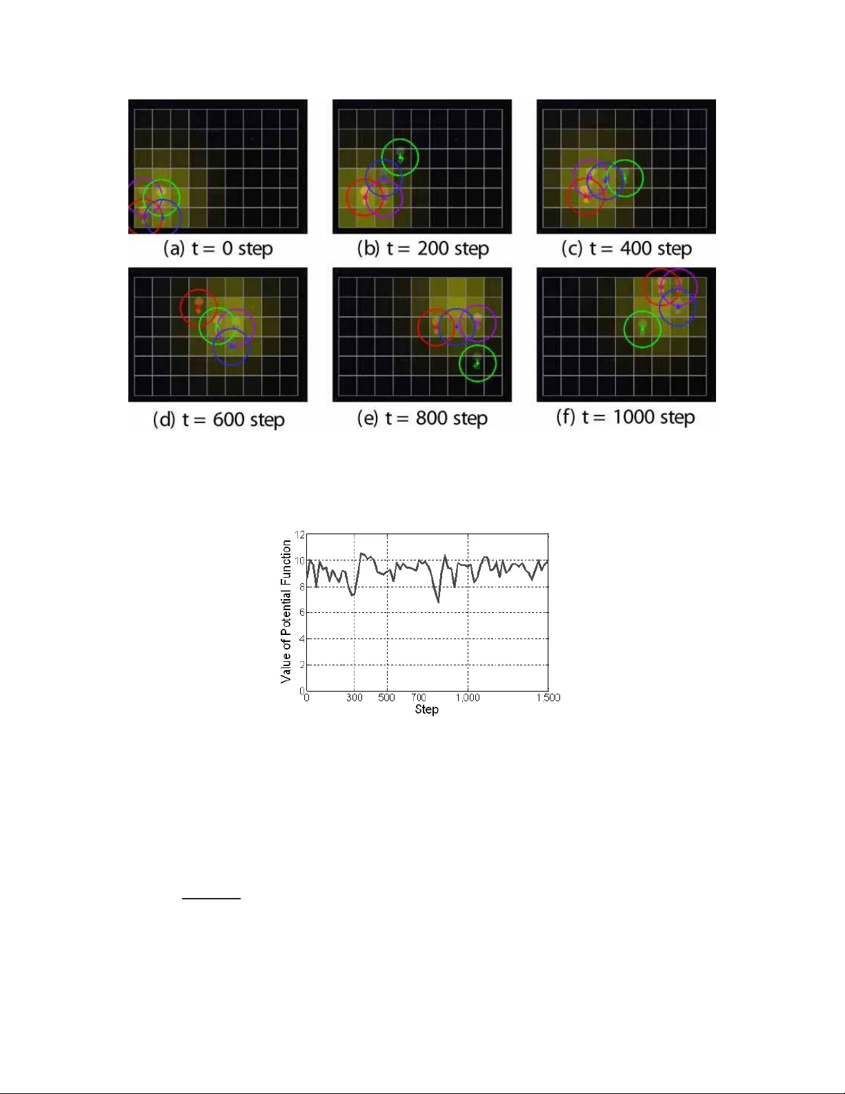
1 P ayof f-based Inhomogeneous P artiall y Irrati onal Play for Potential Game Theoretic Cooperati v e Con trol of Multi-agent Systems T atsuhiko Goto, T akeshi Hatana ka, Member , IEEE and Ma sayuki Fujita, Me mber , IEEE Abstract This paper han dles a kind of strategic game called po tential games and develops a novel learn ing algorithm P ay off-based Inh omogen eous Partially Irrationa l Play (PIPIP). The pre sent algorithm is based on Distributed Inho mogen eous Sy nchron ous Learning (DISL) presented in an existing work but, unlike DISL, PIPIP allo w s agents to make irrational decisions with a specified probability , i.e. agents can choose an action with a lo w utility from the past ac tions stored in the memory . Du e to th e irrational decisions, we can prove conv ergence in probability of c ollectiv e actions to poten tial fu nction m aximizers. Finally , we demonstra te the effecti veness of the present algorithm throug h expe riments on a sensor coverage problem . It is revealed throu gh the demo nstration th at the present lear ning algorithm successfully lead s agents to around po tential function maximizers even in th e p resence of undesirab le Nash eq uilibria. W e also see th rough th e exper iment with a moving de nsity fun ction that PIPIP has adaptability to en viron mental changes. Index T erms potential game, learn ing algorith m, coop erativ e control, mu lti-agent system T atsuhik o Goto is with T oshiba Corporation, T akesh i Hatanaka(correspond ing author) and Masayu ki Fujit a are with the Department of Mec hanical and Control Engineering, T ok yo Institute of T echnology , T ok yo 152-8550 , JAP AN, hatana ka@ctrl.t itech.ac.jp , fu jita@ctr l.titech. ac.jp Nov ember 6, 2018 DRAFT 2 I . I N T R O D U C T I O N Cooperativ e control of multi-agent systems basically aims at desi gning local interactions of agents in order to meet som e glob al objective of t he group [1], [2]. It is also required depending on scenarios that agents achieve the gl obal objective under imperfect prior knowledge on en vi- ronments whil e adapting to the network and en vironmental changes. Nev ertheless, con ventional cooperativ e control schemes do not always embody such functions . For example, in sensor deployment or coverage , mos t of the cont rol s chemes as in [3], [4], [5] assume prior knowledge on a densit y function defined over a missio n space and hence are hardly applicable t o the mission over unknown surroundi ngs. A game theoretic framew ork as in [6] holds tremendous potential for overcoming the drawback of the con ventional schemes. A game theoreti c approach to cooperative control form ulates the problems as non-cooperative games and identifies the objectiv e in cooperative con trol with arri val at some s pecific Nash equilibria [6], [7], [8]. In particular , it is sho wn by J. Marden et al. [ 6] that a v ariety of cooperati ve control problems are related t o so-called potent ial games [9]. Unlike the other game t heory , potential games give a design p erspecti ve, whi ch consists of two kinds of desig n problem: utilit y design and learning algorithm design [10]. T he objective of uti lity design is to al ign local ut ility functions t o be maximi zed by each agent so that t he result ing game constitutes a potent ial game, where the literature [11], [12] provides general design methodologi es. The learning algorit hm design determines action selection rules of agents so that the actions con ver ge to Nash equilib ria. In this paper , we focus on the learning algo rithm desi gn for coop erati ve control of mu lti-agent systems. A l ot of learning algorithm s ha ve been established in game theory literature and recently some alg orithms are also developed mainl y by J. Marden and h is collabo rators. The algorith ms therein are classified into sever al categories dependi ng on their features. The first issue is whether an algorithm presum es finite or infinit e memories. For example, Fictitious Play (FP) [13], Re gret Mat ching (RM) [14], Joint Strategy Fictitious Play (JSFP) with Inerti a [15] and Regret-Based Dynamics [16] require infinit e number of memories for exe cuting the algorithms. M eanwhile, Adaptive Play (AP) [17], Better Reply Process with Finite Memory and Inertia [18], (Restricti ve) Spa tial Adaptive Play ((R )SAP) [19], [6] and Payof f-based Dynamics (PD) [20], Payof f-based version of Log-Linear Learning (PLLL) [21] and Dist ributed Inhomogeneous Synchronous Learning (DISL) [7] require o nly a finite numb er of memories. Of Nov ember 6, 2018 DRAFT 3 course, the finite m emory algorithms are m ore p referable for practical app lications. The second issue is what information is necessary for executing learning al gorithms. For example, FP presum es that all the inform ation of the other agents ’ actio ns are av ailable, which strongly restricts its applications . On th e other hand, RM, JSFP with Inertia and (R)SAP assume a vailability of a s o-called virtual payoff , i .e. the uti lity which would b e obtained if an agent chose an action . Moreover , PD, PLLL and DISL utilize only t he actual payoffs obtained after taking actions, which h as a potential to overcome t he aforementioned drawback of the sensor cove rage schemes [7]. The main objective of standard game th eory is to compute Nash equilibria and hence most of the above algorith ms exce pt for [6], [21] assure only con vergence to pure Nash equilibria. Howe ver , in most of cooperative control prob lems, it i s insufficient for achie ving the global objective and selection of the m ost ef ficient equilibria is required [21]. In this paper , we thus deal with con ver gence of the actions to the Nash equil ibria m aximizing the potential function which are call ed opt imal Nash equ ilibria in thi s paper , s ince th e potential fun ction is usuall y designed in m any cooperative control problems so that its maxi mizers coincide with the actio n profiles achieving the gl obal objectives. The prim ary contribution o f this paper is to d e velop a novel l earning algo rithm called P a yoff- based Inhomogeneous P a rtially Irrational Play (PIPIP ). The learning algorithm is based on DISL presented in [7] and i nherits its seve ral desirable features: (i) The algori thm requires finite and a littl e m emory , (ii) The algorithm is payoff -based, (iii) The algorith m allows agents t o choose acti ons i n a syn chronous fashion at each iteration, (iv) The actio n selectio n procedure in PIPIP consis ts of sim ple rules, (v) The algorithm is capable of dealing with constraint s on action selection. The main difference of PIPIP from DISL is to allow agents to make i rrational decisions with a certain probabili ty , whi ch renders agents opport unities to escape from undesirable Nash equilibria. Thanks to the irratio nal decisions , PIPIP assures th at the actions of the g roup con ver g e in probability to op timal Nash equi libria, though only conv er gence to a pure Nash equilibri um is proved in [7]. M eanwhile, som e learning algorithms as in [6], [21] dealing w ith con ver gence to the optim al Nash equilibria ha ve been presented and we also mention the advantages of PIPIP over these learning algo rithms in the following. RSAP [6] gu arantees con vergence of t he distribution of actio ns t o a stati onary distribution such that the probabi lity stayi ng the optim al Nash equil ibria is arbitrarily specified b y a design parameter . Howe ver , RSAP is not synchronou s Nov ember 6, 2018 DRAFT 4 and virtual payoff-based and hence its applications are restricted. PLLL [21] also allo ws irrational and exploration decisions si milarly to PIPIP and the resulting conclu sion is alm ost compatible with this paper . Howev er , in [21], how to handle the action constraints is not explicit ly shown and con ver gence in probability to the optimal Nash equil ibria is not proved in a strict sens e. The secondary contribution of this paper is to d emonstrate the eff ectiv eness of the present learning algorithm through experiments on a sensor coverage problem, where the learning algorithm is applied to a robotic system compensated by local controllers and logics. Such in vestigatio ns have not been suffic iently addressed in th e existing works. Here, we mainly check the performance o f the l earning algo rithm in finite tim e and adaptabi lity to en vironmental changes. In order to deal with the former issue, we prepare obstacles i n the miss ion space to generate apparent undesirable Nash equilibria. Then, we compare the performance of PIPIP with DISL. The results therein will support our claim that what this paper provides is not a minor extension of [7] and contains a signi ficant contribution from a practical point of view . W e next demons trate the adaptability by employing a moving densit y function defined over the mission space. Though adaptation to time-varying density is in principle expected for payof f- based algorithms, its demo nstration has not been addressed in p re vious works. W e see from the results that desirable group b eha viors, i.e. tracking to the moving high density region are achie ved b y PIPIP eve n in the absence of any knowledge on the density . This paper is organized as follows: In Section II, we give s ome termino logies and b asis necessary for statin g the resul ts of t his paper . In Section III, we present the learning algorithm PIPIP and state the main result associated with the algorithm, i. e. con vergence in probability to the optimal Nash equil ibria. Then, Section IV gives the proof of th e main result. In Section V, we demonstrate the effecti veness o f PIPIP throu gh experiments on a sensor coverage problem. Finally , Section VI draws conclusions. I I . P R E L I M I N A RY A. Constrained P otential Ga mes In this paper , we con sider a constrained st rategic game Γ = ( V , A , { U i ( · ) } i ∈V , {R i ( · ) } i ∈V ) . Here, V := { 1 , · · · , n } is th e set of agents’ unique ident ifiers. The set A is called a collective action set and defined as A := A 1 × · · · × A n , where A i , i ∈ V is the set o f actions which agent i can take. The function U i : A → R is a so-called utility functi on of agent i ∈ V and each Nov ember 6, 2018 DRAFT 5 agent basically beha ves so as to maxi mize t he function. T he function R i : A i → 2 A i provides a so-called constrained action set and R i ( a i ) is the set of actions which agent i wil l be able to take in case he takes an action a i . Namely , at each iteration t ∈ Z + := { 0 , 1 , 2 , · · · } , each agent chooses an action a i ( t ) from the set R i ( a i ( t − 1)) . Throughout this paper , we denote coll ection of actions oth er than agent i by a − i := ( a 1 , · · · , a i − 1 , a i +1 , · · · , a n ) . Then, th e jo int action a = ( a 1 , · · · , a n ) ∈ A is described as a = ( a i , a − i ) . Let us now make the following assumpt ions. Assumption 1 The functio n R i : A i → 2 A i satisfies the following three conditions . • (Re versibil ity [6]) For any i ∈ V and any actions a 1 i , a 2 i ∈ A i , the inclusion a 2 i ∈ R i ( a 1 i ) is equiv alent to a 1 i ∈ R i ( a 2 i ) . • (Feasibility [6]) For any i ∈ V and any actio ns a 1 i , a m i ∈ A i , there exists a sequence of actions a 1 i → a 2 i → · · · → a m i satisfying a l i ∈ R i ( a l − 1 i ) for all l ∈ { 1 , · · · , m } . • For any i ∈ V and any action a i ∈ A i , the num ber of a vailable actions i n R i ( a i ) is greater than or equal t o 3 . Assumption 2 For any ( a, a ′ ) satisfying a ′ i ∈ R i ( a i ) and a − i = a ′ − i , the inequalit y U i ( a ′ ) − U i ( a ) < 1 holds true for all i ∈ V . Assumptio n 2 m eans that when onl y o ne agent changes his action, the difference in the util ity function U i should be smaller th an 1 . This assum ption is satisfied by just scaling all agent s’ utility functions appropri ately . Let us now i ntroduce the potential games under consideration in thi s paper . Definition 1 (Constrained Potential G ames [6], [7]) A constrained strategic game Γ is said to be a cons trained potential game wit h potential function φ : A → R i f for all i ∈ V , e very a i ∈ A i and e very a − i ∈ Q j 6 = i A j , the following equati on holds for every a ′ i ∈ R i ( a i ) . U i ( a ′ i , a − i ) − U i ( a i , a − i ) = φ ( a ′ i , a − i ) − φ ( a i , a − i ) (1) Throughout this paper , we suppose that a potential function φ is designed so that its maximizers coincide with t he joint action a achieving a g lobal objective of the group. Under the situati on, Nov ember 6, 2018 DRAFT 6 (1) im plies that if an agent changes his action, the change of the local objective function i s equal to that of the group objective function. W e next define the Nash equilibria as bel o w . Definition 2 (Constrained Nash Equillibria) For a constrained strategic game Γ , a collection of action s a ∗ ∈ A is said t o be a con strained pure Nash equi librium if the fol lowing equation holds for all i ∈ V . U i ( a ∗ i , a ∗ − i ) = max a i ∈R i ( a ∗ i ) U i ( a i , a ∗ − i ) (2) It is known [7], [9] t hat any constrain ed p otential game h as at least one pure Nash equilibrium and, in particular , a potential function maximizer is a Nash equilibrium, which is called an optimal Nash equilib rium in thi s p aper . Howe ver , t here may exist undesirable pure Nash equilibria not maximizing the potential funct ion. In o rder to reach the optimal Nash equil ibria while av oiding undesirable equilibria, we have to design appropriately a learning algori thm which determines how to select an action at each i teration. B. Resistance T r ee Let us consid er a Markov process { P 0 t } defined ove r a finite state space X . A perturbation of { P 0 t } i s a Markov process whose transitio n probabilities are sli ghtly perturbed. Specifically , a perturbed Markov process { P ε t } , ε ∈ [0 , 1] is defined as a process such t hat t he transi tion of { P ε t } follows { P 0 t } with probabi lity 1 − ε and d oes not follow with p robability ε . Then, we introduce a notio n of r e gular pertu rbation as below . Definition 3 (Regular Pertu rbation [19]) A family of stochastic processes { P ε t } is called a regular perturbation o f { P 0 t } if the fol lowing conditions are satisfied: (A1) For s ome ε ∗ > 0 , the process { P ε t } is irreducible and aperiodic for all ε ∈ (0 , ε ∗ ] . (A2) Let us d enote by P ε xy the transiti on p robability from x ∈ X to y ∈ X along with the Markov process { P ε t } . Then, lim ε → 0 P ε xy = P 0 xy holds for all x, y ∈ X . (A3) If P ε xy > 0 for so me ε , then there exists a real number χ ( x → y ) ≥ 0 such that lim ε → 0 P ε xy ε χ ( x → y ) ∈ (0 , ∞ ) , (3) where χ ( x → y ) is called r esistance of transiti on from x t o y . Nov ember 6, 2018 DRAFT 7 Remark that, from (A1), if { P ε t } is a regular perturbation of { P 0 t } , t hen { P ε t } has the uniqu e stationary distribution µ ( ε ) for each ε > 0 . W e next introduce th e r esistance λ ( r ) of a path r from x ∈ X to x ′ ∈ X along with transiti ons x (0) = x → x (2) → · · · → x ( m ) = x ′ as the value satisfying lim ε → 0 P ε ( r ) ε λ ( r ) ∈ (0 , ∞ ) , (4) where P ε ( r ) denotes the prob ability of th e sequence of transitions. Then, it i s easy to confirm that λ ( r ) is simply given by λ ( r ) = m − 1 X i =0 χ ( x ( i ) → x ( i +1) ) . (5) A s tate x ∈ X is s aid t o com municate wit h state y ∈ X if bot h x y and y x hold, where the notation x y im plies that y is accessible from x i.e. a process starting at st ate x has non-zero probabilit y of transitio ning into y at some p oint. A re curr ent communication class is a class s uch that eve ry pair of states in the class commun icates with each o ther and no st ate outside the class is accessible to the class. Now , let H 1 , · · · , H J be recurrent comm unication classes o f Marko v process { P 0 t } . T hen, wit hin each class, there is a path wi th zero resist ance from every state to every other . In case of a perturbed Marko v process { P ε t } , t here m ay exist sev eral paths from states in H l to states in H k for any two di stinct recurrent communicatio n classes H l and H k . The m inimal resistance among all su ch paths is denoted by χ lk . Let u s n o w define a weighted complete di rected graph G = ( H , H × H , W ) over the recurrent communication class es H = { H 1 , · · · , H J } , where the weight w lk ∈ W of each edge ( H l , H k ) is equal to the min imal resistance χ lk . W e next define l -tr ee which is a spannin g tree ov er G with a root no de H l ∈ H . W e also denot e by G ( l ) the set of all l -trees. The r esist ance of an l -t r ee is the sum of the weights on all the edges of the tree. The stochastic p otential of th e recurrent commu nication class H l is the min imal resistance among al l l -trees in G ( l ) . W e also introduce the not ion of stochastically st able state as below . Definition 4 (Stochastically Stable State [19]) A s tate x ∈ X is said to be stochastically stable, if x satisfies lim ε → 0+ µ x ( ε ) > 0 , where µ x ( ε ) is the value of an element of stationary distribution µ ( ε ) correspondi ng to state x . Using th e above terminol ogies, we introd uce the following well known result which conn ects the stochasti cally stabl e s tates and stochasti c pot ential. Nov ember 6, 2018 DRAFT 8 Pr oposition 1 [19 ] Let { P ε t } be a regular perturbation of { P 0 t } . Then lim ε → 0+ µ ( ε ) exists and the limitin g di stribution µ (0) is a statio nary distribution of { P 0 t } . Moreover t he sto chastically stable states are contai ned i n the recurrent comm unication classes with minim um st ochastic pot ential. C. Er godicit y Discrete-time M arkov processes can be d ivided int o two types: time-homog eneous and time- inhomogeneous, where a M arko v process { P t } is said to be time-hom ogeneous i f the transition matrix denot ed by P t is independent of the t ime and to be a time-inhomogeneous if it is tim e dependent. W e also denote the probability of the state transition from time k 0 to tim e k by P ( k 0 , k ) = Q k − 1 t = k 0 P t , 0 ≤ k 0 < k . For a Markov process { P t } , we in troduce the notion of ergodicity . Definition 5 (Strong Ergodicity [23]) A Markov process { P t } i s said to be strongl y ergodic if there exists a st ochastic vector µ ∗ such that for any distribution µ o n X and t ime k 0 , we ha ve lim k →∞ µP ( k 0 , k ) = µ ∗ . Definition 6 (W eak Ergodicity [23]) A Markov process { P t } is said to be weakly ergodic i f the following equation hol ds. lim k →∞ ( P xz ( k 0 , k ) − P y z ( k 0 , k )) = 0 ∀ x, y , z ∈ X , ∀ k 0 ∈ Z + If { P t } is strongly ergodic, the di stribution µ conv er ges to the un ique distribution µ ∗ from any initial state. W eak ergodicity implies that the information on the initial state vanishes as tim e increases tho ugh con ver gence of µ may not b e guaranteed. Note that the notions of weak and strong ergodicity are equiv alent in case of tim e-homogeneous Markov processes. W e finally in troduce the following well -known resul ts on ergodicity . Pr oposition 2 [23 ] A Markov process { P t } is strongly er godic if the following condi tions hold: (B1) The Markov process { P t } is weakly er godic. (B2) F or each t , th ere exists a stochastic vector µ t on X such that µ t is the left eigen vector of the transiti on matrix P ( t ) with eigen value 1. (B3) The eigen vector µ t in (B2) satisfies P ∞ t =0 P x ∈X | µ t x − µ t +1 x | < ∞ . Moreover , if µ ∗ = lim t →∞ µ t , then µ ∗ is the vector in Definiti on 5. Nov ember 6, 2018 DRAFT 9 I I I . L E A R N I N G A L G O R I T H M A N D M A I N R E S U LT In this section, we present a l earning algorit hm called P ayof f-based Inh omogeneous P arti ally Irrational Play (PIPIP) and state the main result of this paper . At each iteration t ∈ Z + , the learning algorit hm chooses an action according to the foll o wing procedure assum ing that each agent i ∈ V stores previous two chosen actions a i ( t − 2) , a i ( t − 1) and t he out comes U i ( a ( t − 2)) , U i ( a ( t − 1 )) . Each agent first updates a parameter ε called exploration rate by ε ( t ) = t − 1 n ( D + 1) , (6) where D is defined as D := max i ∈V D i and D i is the min imal num ber of steps required for transitionin g between any two actions of agent i . Then, each agent compares the values of U i ( a ( t − 1)) and U i ( a ( t − 2)) . If U i ( a ( t − 1 ) ) ≥ U i ( a ( t − 2)) holds , then he chooses action a i ( t ) according t o the rule: • a i ( t ) is random ly chosen from R i ( a i ( t − 1)) \ { a i ( t − 1) } wi th probabili ty ε ( t ) , (it is called an exploratory decision). • a i ( t ) = a i ( t − 1) with probabilit y 1 − ε ( t ) . Otherwise ( U i ( a ( t − 1 )) < U i ( a ( t − 2 )) ), action a i ( t ) is chosen according to the rule: • a i ( t ) i s randomly chosen from R i ( a i ( t − 1)) \ { a i ( t − 1) , a i ( t − 2) } with probabilit y ε ( t ) (it is called an e xploratory decision). • a i ( t ) = a i ( t − 1) with probabilit y (1 − ε ( t )) ( κ · ε ( t ) ∆ i ) , ∆ i := U i ( a ( t − 2 )) − U i ( a ( t − 1)) (7) (it is called an irrational decis ion). • a i ( t ) = a i ( t − 2) with probabilit y (1 − ε ( t )) ( 1 − κ · ε ( t ) ∆ i ) . (8) The parameter κ should be chosen s o as to s atisfy κ ∈  1 C − 1 , 1 2 i , C := max i ∈V max a i ∈A i |R i ( a i ) | , (9) where |R i ( a i ) | is the number o f elements of the set R i ( a i ) . It is clear under the third item of Assumptio n 1 that the action a i ( t ) is well-defined. Nov ember 6, 2018 DRAFT 10 Algorithm 1 Payoff-based Inhomogeneous Partially Irrational Play (PIPIP) Initialization: Action a is chosen randomly from A . Set a 1 i ← a i , a 2 i ← a i , U 1 i ← U i ( a ) , U 2 i ← U i ( a ) , ∆ i ← 0 for all i ∈ V and t ← 2 . Step 1: ε ← t ( − 1 / ( n ( D +1))) . Step 2: If U 1 i ≥ U 2 i , then set a tmp i ←    rnd( R i ( a 1 i ) \ { a 1 i } ) , w .p. ε a 1 i , w .p. 1 − ε . Otherwise, set a tmp i ←          rnd( R i ( a 1 i ) \ { a 1 i , a 2 i } ) , w .p. ε ( t ) a 1 i , w .p. (1 − ε )( κ · ε ∆ i ) a 2 i , w .p. (1 − ε )(1 − κ · ε ∆ i ) . Step 3: Execute the selected action a tmp i and recei ve U tmp i ← U i ( a tmp ) . Step 4: Set a 2 i ← a 1 i , a 1 i ← a tmp i , U 2 i ← U 1 i , U 1 i ← U tmp i and ∆ i ← U 2 i − U 1 i . Step 5: t ← t + 1 and go to Step 1 . Finally , each agent i exec utes the selected action a i ( t ) and compu tes the resulting utilit y U i ( a ( t )) vi a feedbacks from en vironment and neighboring agents. At the next it eration, agent s repeat the same procedure. The algorithm PIPIP is compactly described in Algo rithm 1, where t he function rnd( A ′ ) outputs an action chosen random ly from the set A ′ . Note that the algorit hm with a const ant ε ( t ) = ε ∈ (0 , 1 / 2] is called P ayoff-based Homogeneous P artially Irrational Play (PHPIP) , which will be us ed for the proof of the main result of th is paper . PIPIP is developed based on the learning algorithm DISL presented in [7]. T he main difference of PIPIP from DISL is t hat agents may choose the action wit h the lower uti lity in Step 2 with probability (1 − ε )( κ · ε ∆ i ) wh ich depends on the diffe rence of the last two s teps’ u tilities ∆ i and the p arameters κ and ε . Thanks to the irrational d ecisions, agents can escape from undesi rable Nash equili bria as wi ll be proved in t he next section. W e are now ready to st ate t he main result of this paper . Before ment ioning it, we define B := { ( a, a ′ ) ∈ A × A| a ′ i ∈ R i ( a i ) ∀ i ∈ V } . (10) Nov ember 6, 2018 DRAFT 11 and ζ (Γ) as the set of t he optimal Nash equilibri a, i.e. potential function maxim izers, of a constrained potential game Γ . Theor em 1 Consi der a const rained potenti al game Γ satisfyi ng Assumpt ions 1 and 2. Suppose that each agent behaves according to Algorit hm 1. Then, a M arko v process { P t } is defined over the space B and the following equ ation is sati sfied. lim t →∞ Prob [ z ( t ) ∈ diag ( ζ (Γ)) ] = 1 , (11) where z ( t ) := ( a ( t − 1) , a ( t )) and dia g( A ′ ) = { ( a, a ) ∈ A × A| a ∈ A ′ } , A ′ ⊆ A . Equation (11) means that the probabil ity that agents ex ecuting PIPIP take one o f the potential function maximi zers con ver ge to 1 . The proof of th is theorem will be shown in the next section. In PIPIP , the p arameter ε ( t ) is u pdated by (6) to prove th e above theorem, which is t he same as DISL. Howe ver , this update rule takes long time to reach a suffic iently small ε ( t ) when the size o f the game, i.e. n ( D + 1) is large. Thus, from the practical point of view , we migh t have t o decrease ε ( t ) based on heurist ics or u se PHPIP with a sufficiently smal l ε . Even in s uch cases, the following theorem at least holds s imilarly to the paper [20 ]. Theor em 2 Consi der a const rained potenti al game Γ satisfyi ng Assumpt ions 1 and 2. Suppose that each agent behaves acc ording to PHPIP . Then, given any probability p < 1 , if the exploration rate ε is s uf ficiently small, for all sufficiently large time t ∈ Z + , the fol lowing equation holds. Prob [ z ( t ) ∈ diag ( ζ (Γ)) ] > p. (12) Theorem 2 assures that the optimal actions are eventually s elected with high probabil ity as long as the final value of ε ( t ) is s uf ficiently small irrespective of the decay rate of ε ( t ) . I V . P RO O F O F M A I N R E S U LT In this section, we prove the main result of this paper (Th eorem 1 ). W e first consi der PHPIP with a const ant exploration rate ε . The state z ( t ) = ( a ( t − 1) , a ( t )) for PHPIP wit h ε consti tutes a perturbed Markov process { P ε t } on the state sp ace B = { ( a, a ′ ) ∈ A × A| a ′ i ∈ R i ( a i ) ∀ i ∈ V } . In terms of t he Markov process { P ε t } induced by PHPIP , the foll o wing lemma holds. Lemma 1 The Markov p rocess { P ε t } induced by PHPIP applied to a const rained p otential game Γ is a regular perturbati on of { P 0 t } under As sumption 1. Nov ember 6, 2018 DRAFT 12 Pr oof : Consider a feasible trans ition z 1 → z 2 with z 1 = ( a 0 , a 1 ) ∈ B and z 2 = ( a 1 , a 2 ) ∈ B and partitio n the set of agents V according to their behaviors along with the transit ion as Λ 1 = { i ∈ V | U i ( a 1 ) ≥ U i ( a 0 ) , a 2 i ∈ R i ( a 1 i ) \ { a 1 i }} , Λ 2 = { i ∈ V | U i ( a 1 ) ≥ U i ( a 0 ) , a 2 i = a 1 i } , Λ 3 = { i ∈ V | U i ( a 1 ) < U i ( a 0 ) , a 2 i ∈ R i ( a 1 i ) \ { a 0 i , a 1 i }} , Λ 4 = { i ∈ V | U i ( a 1 ) < U i ( a 0 ) , a 2 i = a 1 i } , Λ 5 = { i ∈ V | U i ( a 1 ) < U i ( a 0 ) , a 2 i = a 0 i } . Then, the probabil ity of the transi tion z 1 → z 2 is represented as P ε z 1 z 2 = Y i ∈ Λ 1 ε |R i ( a 1 i ) | − 1 × Y i ∈ Λ 2 (1 − ε ) × Y i ∈ Λ 3 ε |R i ( a 1 i ) | − h i × × Y i ∈ Λ 4 (1 − ε ) κε ∆ i × Y i ∈ Λ 5 (1 − ε )(1 − κε ∆ i ) , (13) where h i = 1 i f a 0 i = a 1 i and h i = 2 otherwise. W e see from (13) that th e resistance o f transiti on z 1 → z 2 defined in (3) is given b y | Λ 1 | + | Λ 3 | + P i ∈ Λ 4 ∆ i since 0 < lim ε → 0 P ε z 1 z 2 ε | Λ 1 | + | Λ 3 | + P i ∈ Λ 4 ∆ i = Y i ∈ Λ 1 1 |R i ( a 1 i ) | − 1 Y i ∈ Λ 3 1 |R i ( a 1 i ) | − h i × κ | Λ 4 | < + ∞ (14) holds. Thus, (A3) in Definit ion 3 is satisfied. In add ition, it is straightforward from the procedure of PHPIP to confirm the condit ion (A2) . It is thus sufficient to check (A1) in Definition 3. From the rule of taking exploratory actions in Algorithm 1 and the second item of Assumption 1, we immedi ately see that the set of the stat es accessible from any z ∈ B i s equal to B . This i mplies that the perturbed Markov process { P ε t } is i rreducible. W e next check aperiodi city of { P ε t } . It is clear t hat any s tate i n diag( A ) = { ( a, a ) ∈ A × A| a ∈ A } has period 1 . Let us next pi ck any ( a 0 , a 1 ) from the s et B \ diag( A ) . Since a 0 i ∈ R i ( a 1 i ) holds iff a 1 i ∈ R i ( a 0 i ) from A ssumption 1, the following two paths are both feasible: ( a 0 , a 1 ) → ( a 1 , a 0 ) → ( a 0 , a 1 ) , ( a 0 , a 1 ) → ( a 1 , a 1 ) → ( a 1 , a 0 ) → ( a 0 , a 1 ) . This implies that t he period of state ( a 0 , a 1 ) is 1 and the process { P ε t } i s proved to be aperiodic. Hence the process { P ε t } is both i rreducible and aperiodic, which means (A1) in Definitio n 3. In summary , condition s (A1) – (A3) in Definition 3 are sat isfied and the proof is compl eted. From Lemma 1, the p erturbed Markov process { P ε t } is irreducible and h ence there exists a unique st ationary dist ribution µ ( ε ) for ev ery ε . Moreover , because { P ε t } i s a regular perturbation Nov ember 6, 2018 DRAFT 13 of { P 0 t } , we see from the former h alf of Proposition 1 that lim ε → 0+ µ ( ε ) exists and the li miting distribution µ (0) is the stationary di stribution of { P 0 t } . W e also have t he fo llowing lemma on the Markov process { P ε t } induced by PHPIP . Lemma 2 Consider the Markov process { P ε t } induced by PHPIP applied to a constrained potential game Γ . Then, t he recurrent com munication classes {H i } o f the unperturbed Markov process { P 0 t } are giv en by elem ents of diag ( A ) = { ( a, a ) ∈ A × A| a ∈ A} , namely H i = { ( a i , a i ) } , i ∈ 1 , · · · , |A| . (15) Pr oof : Because of the rule at Step 2 of PHPIP , it is clear that any state belonging to diag ( A ) cannot move to another s tate without explorations, which im plies that al l the st ates in diag ( A ) itself form recurrent com munication classes of the unperturbed Markov process { P 0 t } . W e n ext consider the states i n B \ diag( A ) and prove that these s tates are n e ver included in recurrent communication cl asses of t he unperturbed Marko v process { P 0 t } . Here, we use induction. W e first consider the case of n = 1 . If U 1 ( a 1 1 ) ≥ U 1 ( a 0 1 ) , then the transition ( a 0 1 , a 1 1 ) → ( a 1 1 , a 1 1 ) i s taken. Otherwise, a sequence of transitio ns ( a 0 1 , a 1 1 ) → ( a 1 1 , a 0 1 ) → ( a 0 1 , a 0 1 ) o ccurs. Thus, in case of n = 1 , the state ( a 0 1 , a 1 1 ) ∈ B \ diag ( A ) is never included in recurrent com munication classes of { P 0 t } . W e next make a hypothesi s that there exists a k ∈ Z + such th at all the states i n B \ diag ( A ) are n ot i ncluded in recurrent communication classes of the unperturbed Marko v process { P 0 t } for all n ≤ k . Then, we consider the case n = k + 1 , where there are three pos sible cases: (i) U i ( a 1 ) ≥ U i ( a 0 ) ∀ i ∈ V = { 1 , · · · , k + 1 } , (ii) U i ( a 1 ) < U i ( a 0 ) ∀ i ∈ V = { 1 , · · · , k + 1 } , (iii) U i ( a 1 ) ≥ U i ( a 0 ) for l agents where l ∈ { 2 , · · · , k } . In case (i), the transiti on ( a 0 , a 1 ) → ( a 1 , a 1 ) must occur for ε = 0 and, i n case (ii), the transition ( a 0 , a 1 ) → ( a 1 , a 0 ) → ( a 0 , a 0 ) should be selected. Thus, all th e states in B \ diag ( A ) satisfyi ng (i) or (ii) are nev er includ ed in recurrent communi cation class es. In case (iii), at t he next it eration, all the agents i satisfyi ng U i ( a 1 ) ≥ U i ( a 0 ) choose the current acti on. Then, such agents possess a single action in the m emory and , in case of ε = 0 , each agent has to choose either of the actions in the m emory . Namely , these agents never change t heir action s in all su bsequent iterations. The resulting situation is thus the same as the case of n = k + 1 − l . From the above hypothesi s, Nov ember 6, 2018 DRAFT 14 we can conclude that the s tates in case (iii) are also not included in recurrent com munication classes. In summ ary , the states in B \ diag( A ) are ne ver included in the recurrent comm unication classes of { P 0 t } . The proof i s thus completed. A feasible path over t he process { P ε t } from z ∈ B to z ′ ∈ B is especially said to be a route if both of the two nodes z and z ′ are element s of diag ( A ) ⊂ B . Note that a rout e is a path and hence the resistance of t he route is als o given by (4). Especially , we define a straight r out e as follows, where we use the not ation E sing le := { ( z = ( a, a ) , z ′ = ( a ′ , a ′ )) ∈ diag ( A ) × diag( A ) | ∃ i ∈ V s.t. a i ∈ R i ( a ′ i ) , a i 6 = a ′ i and a − i = a ′ − i } . (16) Definition 7 (Straight Route) A rou te between any two states z 0 = ( a 0 , a 0 ) and z 1 = ( a 1 , a 1 ) in diag ( A ) su ch that ( z 0 , z 1 ) ∈ E sing le is said to be a straight route i f the path is given by the transitions on the Markov process { P ε t } such that only o ne agent i changes hi s action from a 0 i to a 1 i at first iteration and the explored agent i selects the same action a 1 i at the n ext it eration while the oth er agents choose the s ame action a 0 − i = a 1 − i during the two steps. In terms of t he straight route, we hav e the following lem ma. Lemma 3 Consider paths from any state z 0 = ( a 0 , a 0 ) ∈ diag ( A ) t o any state z 1 = ( a 1 , a 1 ) ∈ diag( A ) such that ( z 0 , z 1 ) ∈ E sing le over the Markov process { P ε t } i nduced by PHPIP appli ed to a constrained pot ential game Γ . Then, under As sumption 2, the resistance λ ( r ) of the straigh t route r from z 0 to z 1 is stri ctly small er than 2 and the resist ance λ ( r ) is minimal amon g all paths from z 0 to z 1 . Pr oof : Along with the straight route, only one agent i first changes action from a 0 i to a 1 i , whose probability i s giv en by (1 − ε ) n − 1 × ε |R i ( a 0 i ) | − 1 . (17) It is easy to confirm from (17) that the resistance of the transition ( a 0 , a 0 ) → ( a 0 , a 1 ) is equal to 1 . W e next con sider the transition from ( a 0 , a 1 ) to ( a 1 , a 1 ) . If U i ( a 1 ) ≥ U i ( a 0 ) is true, the probability of this transition is giv en by ( 1 − ε ) n , whose resistance is equal to 0 . Otherwise, Nov ember 6, 2018 DRAFT 15 U i ( a 1 ) < U i ( a 0 ) holds and the probabili ty of this t ransition is give n by (1 − ε ) n × κε ∆ i , whose resistance is ∆ i . Let us now notice that the resis tance λ ( r ) of the straight route r is equal t o the sum of the resistances of transitions ( a 0 , a 0 ) → ( a 0 , a 1 ) and ( a 0 , a 1 ) → ( a 1 , a 1 ) from (5) and that ∆ i < 1 from Assumption 2. W e can thus conclude that λ ( r ) is smaller than 2 . It is also easy t o confirm that the resi stance of paths such that more than 1 agents t ake exploratory action shou ld be greater than 2 . Namely , the straight route gives the sm allest resistance among all paths from z 0 = ( a 0 , a 0 ) to z 1 = ( a 1 , a 1 ) and hence the proof is com pleted. W e also i ntroduce the following no tion. Definition 8 ( m -Straight-Route) An m -straight-route is a route which passes t hrough m ver - tices in diag ( A ) and al l the routes between any two of these vertices are straight. In terms of the route, we can prove th e foll owing lemma, which clarifies a conn ection between the potenti al function and the resistance of the route. Lemma 4 Consider th e Markov process { P ε t } induced by PHPIP applied to a constrained poten- tial game Γ . Let us denote an m -straight-route r ove r { P ε t } from state z 0 = ( a 0 , a 0 ) ∈ diag ( A ) to state z 1 = ( a 1 , a 1 ) ∈ diag ( A ) by z (0) = z 0 ⇒ z (1) ⇒ z (2) ⇒ z (3) ⇒ · · · z ( m − 3) ⇒ z ( m − 2) ⇒ z ( m − 1) = z 1 , (18) where z ( i ) = ( a ( i ) , a ( i ) ) ∈ diag( A ) , i ∈ { 0 , · · · , m − 1 } and all the arro ws between them are straight routes. In addition, we denote its rev erse route r ′ by z (0) = z 0 ⇐ z (1) ⇐ z (2) ⇐ z (3) ⇐ · · · ⇐ z ( m − 3) ⇐ z ( m − 2) ⇐ z ( m − 1) = z 1 , (19) which is also an m -straight rou te from z 0 to z 1 . Then, under Ass umption 2, if φ ( a 0 ) > φ ( a 1 ) , we hav e λ ( r ) > λ ( r ′ ) . Pr oof : W e suppose that th e rou te r contains p straight routes wit h resist ance g reater than 1 and r ′ contains q straight rout es with resis tance greater t han 1 . Let us now denote the explored agent along with the route z ( i ) ⇒ z ( i +1) by j i and that with z ( i ) ⇐ z ( i +1) by j ′ i . From the proof of Lemm a 3, the resistance of the route z ( i ) ⇒ z ( i +1) should be exactly equal to 1 (in case of U j i ( a ( i +1) ) ≥ U j i ( a ( i ) ) ) or equal t o 1 + ∆ j i ∈ (1 , 2) (in case of U j i ( a ( i +1) ) < U j i ( a ( i ) ) ). From (1), the fol lowing equatio n holds. ∆ j i = U j i ( a ( i ) ) − U j i ( a ( i +1) ) = φ ( a ( i ) ) − φ ( a ( i +1) ) = U j ′ i ( a ( i ) ) − U j ′ i ( a ( i +1) ) = − ∆ j ′ i . (20) Nov ember 6, 2018 DRAFT 16 Namely , one of the resistances of the straight routes z ( i ) ⇒ z ( i +1) and z ( i +1) ⇐ z ( i ) is exactly 1 and the other is greater than 1 except for th e case that U i ( a ( i +1) ) = U i ( a ( i ) ) in which the resistances are both equal to 1 . A n illust rati ve example of the relation is giv en as fol lows, where the numb ers pu t on arro ws are th e resistances of the routes. z (0) = z 0 1+∆ j 0 ⇒ z (1) 1 ⇒ z (2) 1+∆ j 1 ⇒ z (3) 1 ⇒ · · · 1 ⇒ z ( m − 3) 1 ⇒ z ( m − 2) 1+∆ j m − 2 ⇒ z ( m − 1) = z 1 z (0) = z 0 1 ⇐ z (1) 1+∆ j ′ 1 ⇐ z (2) 1 ⇐ z (3) 1+∆ j ′ 3 ⇐ · · · 1+∆ j ′ m − 4 ⇐ z ( m − 3) 1+∆ j ′ m − 3 ⇐ z ( m − 2) 1 ⇐ z ( m − 1) = z 1 Namely , the inequality p + q ≤ m − 1 holds true. Let us now col lect all the ∆ j i such that the resistance of z ( i ) ⇒ z ( i +1) is greater t han 1 and number them as ∆ 1 , ∆ 2 , · · · , ∆ p . Similarly , we define ∆ ′ 1 , ∆ ′ 2 , · · · , ∆ ′ q for the rev erse route r ′ . Then, from equations in (20), we obtain ∆ 1 + ∆ 2 + · · · + ∆ p − (∆ ′ 1 + ∆ ′ 2 + · · · + ∆ ′ q ) = φ ( a 0 ) − φ ( a 1 ) . (21) Note that (21) holds ev en in the presence of pairs ( a ( i ) , a ( i +1) ) such that U j i ( a ( i +1) ) = U j i ( a ( i ) ) . Since ∆ 1 + · · · + ∆ p = λ ( r ) − ( m − 1) and ∆ ′ 1 + · · · + ∆ ′ q = λ ( r ′ ) − ( m − 1) from (5), we obtain λ ( r ) = λ ( r ′ ) + φ ( a 0 ) − φ ( a 1 ) . (22) It is straigh tforward from (22) to prove the stat ement in the lemm a. Let u s form t he weighted digraph G over the recurrent communicati on classes for the Markov process { P ε t } induced by PHPIP as in Subsection II-B, where the weight w lk of each edge ( H l , H k ) i s equal to the minim al resistance χ lk among all the paths connecting two recurrent communication classes H l and H k . From Lemma 2, t he nodes of th e graph G are given by each element of the set diag( A ) and hence G = (diag ( A ) , E , W ) , E ⊆ diag ( A ) × diag( A ) . Since all the recurrent communicatio n classes have onl y one element as in (15), th e weight w lk for any two states z l , z k ∈ diag( A ) is s imply given by the path wi th mini mal resistance amo ng al l paths from z l to z k . In addi tion, Lemma 3 proves that if ( z l , z k ) ∈ E sing le , the weight w lk = χ lk is giv en by the resistance of the straig ht route from z l to z k . Let us focus on l -trees ove r G whose root is a state z l ∈ diag( A ) . Recall no w that the resistance of t he tree i s the s um of the wei ghts of all the edges consti tuting the tree as defined in Subsection II-B. Then, we have the fol lowing lemma in terms of the st ochastic p otential of z l , which is the minim al resistance among all l -trees in G ( l ) . Nov ember 6, 2018 DRAFT 17 diag A Kruskal's Algorithm Fig. 1. Image of Kruskal’ s Al gorithm Lemma 5 Consider the weighted directed graph G const ituted from the Markov process { P ε t } i n- duced by PHPIP a pplied to a const rained pot ential game Γ . Let us denote by T = (diag( A ) , E l , W ) the l -tree giving the s tochastic potential of z l ∈ diag( A ) . If Assumpti ons 1 and 2 are satisfied, then the edge s et E l must be a subset of E sing le . Pr oof : The edges of G , denoted by E , are divided into two classes: E s := E sing le and E d := E \ E s . From Lem ma 3, the weights o f the edges in E s are small er than 2 . W e next consi der the weights of the edges in E d . Because of the nature of PHPIP , any agent cannot change h is action to anoth er one witho ut explorations when z ( t ) ∈ diag ( A ) , and hence exploration should be executed more than twice in order that the transit ion along with an edge in E d occurs. Th is implies that th e weig hts of edges i n E d should be greater than 2 . Hereafter , we simpl y re write t he weights o f t he edges E s by w s ( < 2) and t hose of E d by w d ( ≥ 2) and build t he mini mal resistance tree w ith root z l over this s implified graph. Not e that this simpli fication does not change the elements of the edg e set E l . It should be not ed that from Assumptio n 1 all recurrent comm unication classes ( diag ( A ) ) can be connected by passi ng only through s traight routes. From the procedure of Krus kal’ s Algorith m, edges with resistances w d are never chosen as edges o f the minim al tree as illustrated in Fig. 1. Thus, the tree giving the stochastic potenti al must con sist only of the edges in E s , which compl etes t he proof. W e are now ready t o state the following proposition on the stochasti cally stable states (Defi- nition 4) for th e Markov process { P ε t } . Nov ember 6, 2018 DRAFT 18 Optimal Nash Equilibrium Optimal Nash Equilibrium Fig. 2. Resistance T rees (the left t ree should have a greater resistance t han the right) Pr oposition 3 Cons ider { P ε t } induced by PHPIP app lied to a constrained potent ial game Γ . If Assumptio ns 1 and 2 are satisfied, t hen the sto chastically stable states are includ ed in diag( ζ (Γ)) , with the set of the opt imal Nash equilib ria ζ (Γ) . Pr oof : From Proposition 1, Lemm as 1 and 2, it is sufficient to prov e that the st ates in diag( A ) w ith the mi nimal s tochastic potential over G are included in ζ (Γ) . Let us introduce the notations z nonopt = ( a nonopt , a nonopt ) ∈ diag ( A ) with a non opt imal action a nonopt and z opt = ( a opt , a opt ) ∈ diag ( A ) wit h an opt imal Nash equilibrium a opt . If z nonopt is the root of a t ree T , there exists a unique route from z opt to z nonopt over T . From Lemm a 5, the route r is an m -straight-route for some m . Now , we can build a tree T ′ with root z opt such th at only the route r is replaced by its re verse route r ′ (Fig. 2). Then, we have λ ( r ) > λ ( r ′ ) from Lemma 4 since φ ( a opt ) > φ ( a nonopt ) . Thus, the resistance of T ′ is small er than that of T and the stochastic po tential of z opt is small er than the resistance of T ′ . The statement holds regardless of the selection of a nonopt . This completes the proof. W e next consider PIPIP with time-varying ε ( t ) and prove strong ergodicity of { P ε t } . Lemma 6 The Markov process { P ε t } i nduced by PIPIP applied to a constrain ed potential game Γ is strong ly er godic. Pr oof : W e us e Proposition 2 for the proof. Condit ions (B2) , (B3) in Propos ition 2 can b e proved i n t he same way as [7]. W e thus show only t he sati sfaction of Condition (B1) . As in Nov ember 6, 2018 DRAFT 19 (13), the probabili ty of transition z 1 → z 2 is give n b y P ε z 1 z 2 = Y i ∈ Λ 1 ε |R i ( a 1 i ) | − 1 × Y i ∈ Λ 2 (1 − ε ) × Y i ∈ Λ 3 ε |R i ( a 1 i ) | − h i × × Y i ∈ Λ 4 (1 − ε ) κε ∆ i × Y i ∈ Λ 5 (1 − ε )(1 − κε ∆ i ) . (23) Since ε ( t ) is s trictly decreasing, there is t 0 ≥ 1 such that t 0 is the first time when (1 − ε ( t ))(1 − κε ( t ) ∆ i ) ≥ ε ( t ) C − 1 , 1 − ε ( t ) ≥ ε ( t ) (1 − ∆ i ) κ ( C − 1) (24) holds. Note that the existence of ε satisfying (24) is guaranteed from the condition (9). For all t ≥ t 0 , we have P ε z 1 z 2 ( t ) ≥  ε ( t ) C − 1  n . (25) The remaining part of the proof is the same as [7] and o mit it in thi s paper . W e are now ready t o prove Theorem 1 . From Lem ma 6, the distribution µ ( ε ( t )) con ver ges to the uni que distribution µ ∗ from any initial state. In addition, we also h a ve µ ∗ = µ (0) = lim ε → 0 µ ( ε ) from lim t →∞ ε ( t ) = 0 . W e have already p rove d from Propositions 1 and 3 that any state z satisfyin g µ z (0) > 0 mu st be included in dia g ( ζ (Γ)) . Therefore, lim t →∞ Prob[ z ( t ) ∈ diag ( ζ (Γ)) ] = 1 , is proved, which completes the p roof of Theorem 1. Theorem 2 is also proved from Proposit ion 1, Lemma 1 and Proposition 3. V . A P P L I C A T I O N T O S E N S O R C O V E R A G E P RO B L E M In this section we demonstrate th e eff ectiv eness o f the proposed learning algo rithm PIPIP through experiments of the sensor cove rage p roblem in vestigated e.g. in [3], [4], [5] whose objective is t o cover a missi on s pace ef ficiently usi ng d istributed control strategies. In particular , the problem of th is section is form ulated based on [7] wi th some modifications . A. Pr obl em F ormulatio n W e suppos e that the missi on space to be covered is give n by Q c ⊂ R 2 and that a density function W c ( q ) , q ∈ Q c is defined over Q c . In particul ar , to const itute a game i n t he form of the pre vious sections, we also prepare a discretized missio n space Q consistin g of a fini te number Nov ember 6, 2018 DRAFT 20 of poi nts in Q c . Accordingly , we als o define th e discretized version of the densi ty W ( q ) , q ∈ Q such that W ( q ) = W c ( q ) ∀ q ∈ Q . In the problem, th e positi on of agent i in t he miss ion space Q is regarded as the action a i to be determined, and hence the action set A i is give n by a subset of Q for all i ∈ V . Namely , each agent i chooses his action a i from the finite s et A i ⊆ Q at each iteration and move tow ard the corresponding point. Suppose now that each sensor has a limi ted sensing radius r m and that agent i l ocated at a i ∈ Q may sens e an event at q ∈ Q iff q ∈ D ( a i ) := { q ∈ Q| k q − a i k ≤ r m } . W e also denote by n q ( a ) the number of agents such that q ∈ D ( a i ) wh en agents take the join t action a . Then, we define the fun ction φ ( a ) = X q ∈Q n q ( a ) X l =1 W ( q ) l dq . This function means, as n q ( a ) increases, the sensing accurac y at q ∈ Q i mproves b ut the increment decreases, which captures the characteristics of the sensor coverage problem. Note that the authors in [7] take account of energy consumption of sens ors in add ition to cov erage performance and claim that the function φ cannot be a performance measure. Ho wev er , w e do not consider the energy consu mption and what is the best selection of the performance measure depends on the subjective views of desig ners. W e thus id entify maxim ization of φ with the glob al objective of the group lett ing φ be the potential function. Let us now i ntroduce the utility function U i ( a ) = X q ∈D ( a i ) W ( q ) n q ( a ) . Then, equ ation (1) h olds for the above p otential functi on φ [7] and hence a potential game is constituted. It is also easy to confirm th at the utilit y U i ( a ) can be locally computed if we assume feedbacks of W q , q ∈ D ( a i ) from en vironment and of the selected actio ns a j , j 6 = i o nly from neighboring agents specified by the 2 r m -disk proximit y comm unication graph [1]. B. Objectives In this section, we run two experiments whose objectives are l isted below . • Demonstration of effecti veness: Theorems 1 and 2 assure statements after i nfinitely long time but it is required in practice that the algorithm works in finite ti me. The first objective Nov ember 6, 2018 DRAFT 21 Fig. 3. Mobile Robot is t hus to check if the agents s uccessfully cover the miss ion space (i) e ven in the presence of cons traints such as obstacles and mobilit y constraints, and (ii) in the absence of the prior information on the density functi on. The second obj ectiv e is to com pare its performance with the learning algorithm DISL, wh ich is chosen to ensure fair comparisons . Indeed, the other existing alg orithms require either or both of p rior k nowledge on density or free mot ion without constraints. • Adaptability to en vironmental changes: In man y real applications of sensor coverage schemes, it is required for sensors to change the configuration according t o the surrounding en viron- ment. In particular , the dens ity function can be t ime-varying e.g. in the scenario such as measuring of radiati on quantit y in the air and sampling of some chemical material and temperature in the ocean. It is expected for payoff-based algorithm s t o naturall y adapt to such en vironmental changes without alt ering action selection rules and any com plicated decision-making processes due to the characteristics that prior knowledge on en v ironments except for A i is not assumed. W e thus check the fun ction by using a Gaussi an density function whose mean m oves as time advances. C. Experimental System In the experiments, we use four mo bile robots with four wheels which can m ove in any direction (Fig. 3). Fig. 4 shows the schematic of the experimental system. A camera (Firefly MV (V iewPLUS Inc.) with lenses L TV2Z 3314CS-IR (Raymax Inc.)) is m ounted over the field. The image inform ation is sent to a PC and processed to extract the pose of robo ts from the image by the image processing library OpenCV 2.0 . Note that a board with two colored feature point s Nov ember 6, 2018 DRAFT 22 Fig. 4. Experimental Schematic Fig. 5. Setting of Experiment 1 is attached to each robot as in Fig. 3 to help th e extraction. According to the extracted pos es, the actions to be taken by agents are computed based on learning algorithm s. H o wev er , in the experiments, the selected actions are not exe cuted directly s ince col lisions among robots must be a voided. For this pu rpose, a local decision-makin g mechanism checks whether coll isions would occur if th e selected actions were executed. The mechanism i s desi gned based on heuris tics and we av oi d mentioning the details since i t is not essential. If the answer of the mechanism i s yes, the agent s decide to stay at the current position. Otherwis e, the selected action s are sent as reference position s togeth er with t he current poses to the local velocity and position PI controll er implemented o n a di gital signal processor DS-1104 (dSP A CE Inc.). Then, the ev entual velocity command is sent to each robot via a wireless communi cation d e vice X Bee (Digi International Inc.). The following setup is com mon i n all experiments. The mission sp ace Q c := [0 2 . 7 ]m × [0 1 . 8]m is divided into 9 × 6 squares wi th si de length 0 . 3 m as i n Fig. 5 lett ing t he d iscretized set Q be give n b y the centers of the squares as Q = { (0 . 15 + 0 . 3 j, 0 . 15 + 0 . 3 l ) | j ∈ { 0 , · · · , 8 } , l ∈ { 0 , · · · , 5 } } . The sensing radius r m is set as r m = 0 . 3 m for all robots. W e also assume t hat each agent has Nov ember 6, 2018 DRAFT 23 Fig. 6. Configurations by DISL (Experiment 1) a mobili ty const raint R i ( a i ) = { a i ± 0 . 3( b 1 , b 2 ) ∈ A i | b 1 ∈ {− 1 , 0 , 1 } , b 2 ∈ {− 1 , 0 , 1 }} . The initi al actions of agents are s et as a 1 (0) = (0 . 1 5 , 0 . 15) , a 2 (0) = (0 . 1 5 , 0 . 45) , a 3 (0) = (0 . 4 5 , 0 . 15) , a 4 (0) = (0 . 4 5 , 0 . 45) . D. Experiment 1 In the first experiment, we demonstrate the ef fectiv eness of PIPIP . For this purpo se, we em ploy the density function W ( q ) = e − 25 k q − µ k 2 9 , µ = (1 . 95 , 1 . 35) and prepare obstacles at O := { (0 . 7 5 , 1 . 35) , (1 . 05 , 1 . 05) , ( 1 . 35 , 0 . 7 5 ) , (1 . 65 , 0 . 45) } . (26) Namely , in the experiment, the action sets are given by A i = Q \ O . The setup is ill ustrated in Fig. 5, where the region wit h hi gh density is colored by yellow and the red cross mark in dicates Nov ember 6, 2018 DRAFT 24 Fig. 7. Configurations by PIP IP (Experimen t 1) the actions prohibited to b e taken by the obstacles. Un der the situation, we see t hat there exist some Nash undesi rable equil ibria ju st ahead on the left o f the obstacles. It sh ould be also noted that each robot does not know the function W ( q ) a pri ori . W e first run DISL under the above s ituation with the exploration rate ε = 0 . 15 . Th en, th e resulting configurations at 0 , 15 0 , 3 00 , 450 , 600 and 700 steps are shown in Fig. 6. Under the setti ng, three robots cannot reach th e colored region at least in 700 step. It is now easily confirmed that t he configurations at 600 and 70 0 [step] are Nash equili bria only for the three robots and hence they cannot i ncrease utili ties by any one agent’ s acti on change. W e next run PIPIP l etting the parameter ε be fixed as ε = 0 . 1 5 and setting κ = 0 . 5 (namely , PHPIP is actuall y run in th e experiment). Fig. 7 shows resulti ng configurations at the same steps as Fig. 6. Surprisingly , w e see that all the robots ev entually av oid th e obst acles and arrive at the colored region though they initiall y do not k now where is im portant. Such a behavior is nev er achiev ed by con ventional coverage control schemes. The t ime responses of the potent ial function φ for PIPIP and DISL are illust rated in Fig. 8, where the soli d line shows the response for PIPIP and t he dashed line for DISL. As is apparent from the above in vestigations, PIPIP Nov ember 6, 2018 DRAFT 25 Fig. 8. Time E volu tion of Potential F unction f or ε = 0 . 15 (Experiment 1) Fig. 9. T ime E volution of Potential Function f or ε = 0 . 3 (Experiment 1) achie ves a higher potential funct ion value than DISL. Though we can show only o ne samp le due to the page constraints, sim ilar results are obtained for both DISL and PIPIP through sever al trials. From the result s, we claim that PIPIP has a stronger tend ency to escape undesirable Nash equilib ria than DISL, which is also confirmed by the meaning o f the irrational decision. Of course, th e results strongly depend on the value of exploration rate ε . W e thus show the tim e e volution o f th e function φ for ε = 0 . 3 in Fig. 9. W e see from Fig. 9 that some agents executing DISL also do not reach t he important region ev en for ε = 0 . 3 , which seems to be quite high probability as an exploration r ate. Indeed, the fluctuation of the responses is l ar ge and an agent with PIPIP overcomes the obstacle again lea ving t he colored region. From all the above results, we thus can st ate that guarantees of only con ver gence to Nash equil ibria can be a sign ificant problem not only from the theoretical point of view b ut also from the practical vi e wpoint. Though much more thoroug h com parisons are necessary in order to make th e claim on superiority o f PIPIP over DISL confident, PIPIP achieves a better performance than DISL at least in the setup. E. Experiment 2 W e next demonstrate th e adaptabili ty of PIPIP to en v ironmental changes, where we get rid of the obstacle O and hence A i = Q . In th e experiment, we use the following Gaussian density Nov ember 6, 2018 DRAFT 26 Fig. 10. Configurations by P IPIP (E xperiment 2) Fig. 11. T i me Evolu tion of Potential Function (Experiment 2) function whose mean g radually moves. W c ( q ) = e − 25 k q − µ ( t ) k 2 9 , µ ( t ) =          (0 . 45 , 0 . 45) , if t ∈ [0 , 300] (0 . 00375 t − 0 . 6750 , 0 . 00225 t − 0 . 225) , if t ∈ (3 0 0 , 700) (1 . 95 , 1 . 35) , if t ≥ 700 It is worth noting that agents select actions wi thout using any prior information on the densi ty . Nov ember 6, 2018 DRAFT 27 Figs 10 and 11 respectively il lustrate the resulting configurations at 0 , 200 , 400 , 600 , 800 and 1000 steps and tim e evolution of the po tential fun ction φ . W e s ee from Fig. 10 that agents gather at aroun d the most imp ortant region at any ti me ins tant w hile l earning the environmental changes. Fig. 11 also shows that the pot ential function keeps almost t he same l e vel duri ng whole time, which i ndicates that the agents successfull y track the most imp ortant region. From these results, as expected, agent s ex ecuting PIPIP s uccessfully adapt to the en vironmental changes without changing the action selection rule at all. Such a behavior i s also never achiev ed by con ventional covera ge control schem es. V I . C O N C L U S I O N In t his paper , we ha ve developed a ne w learning algo rithm Payoff-based Inhom ogeneous Partially Irrational Play (PIPIP) for p otential game theoreti c cooperativ e control of multi-agent systems. The p resent algorithm is based on Distributed Inhomogeneou s Synchronou s Learning (DISL) presented in [7] and i nherits several desirable features of DISL. Howe ver , un like DISL, PIPIP allows agents to make irrational decisions, that is, take an action giving a lower uti lity from the past two actions. Th anks to the decision, we have succeeded proving con vergence of the joi nt action to the potential functi on maximizers while escaping from undesirable Nash equili bria. Then, we ha ve dem onstrated the utili ty of PIPIP through experiments on a sensor covera ge problem. It has been re vealed through the demons tration that the present learning algorith m w orks e ven in a finite-tim e interval and agents successfully arrive at around the optimal Nash equilibria in the presence of obstacles in the mi ssion sp ace. In addition, we also hav e seen through an experiment with a moving density function that PIPIP has adaptabil ity to en vironment al changes, which is a function expected for payoff-based learnin g algorithms. R E F E R E N C E S [1] F . Bullo, J. Cortes and S. Martinez, Di stributed Contr ol of Robotic Networks , S eries in Applied Mathematics, Princeton Univ ersity Press, 2009. [2] R. M. Murray , “Recent Research in Cooperativ e Control of Multiveh icle Systems, ” Journal of Dynamic Systems Measur ement and Contr ol-T ransactions of The Asme , V ol. 129, No. 5, pp. 571–58 3, 2007. [3] J. Cortes, S .Martinez, T . Karatas and F . Bullo, “Cov erage Control for Mobile Sensing Networks, ” IEEE T rans. on R obotics and Automation , V ol. 20, No. 2, pp. 243–255, 2004. [4] W . Li and C. G. Cassandras, “Sensor Networks and C ooperati ve Control, ” Euro pean Jo urnal of Contro l , V ol. 11, pp. 436–46 3, 2005. Nov ember 6, 2018 DRAFT 28 [5] C. H. Caicedo-N and M. Z efran, “ A Cove rage Algorithm for A Class of Non-co n ve x Re gions, ” in Pr oc. of the 47th IEE E International Confer ence on Decision and Control , pp. 4244– 4249, 2008. [6] J. R . Marden, G. Arslan and J. S . Shamma, “Cooperativ e Control and Potential Games, ” IEEE T rans. on Systems, Man and Cybernetics , V ol. 39, No. 6, pp. 1393–14 07, 2009. [7] M. Zhu and S. Martinez, “Distributed Coverage Games for Mobile V isual Sensor Networks, ” SIAM Journa l on Contr ol and Optimization , subm itted (down loadable at arXi v:1002.036 7 v1), 2010. [8] N. Li and J. R. Marden, “Designing Games to Handle Coupled C onstraints”, in Proc. of t he 49th IE EE Confer ence on Decision and Contro l , pp. 250–2 55, 2010. [9] D. Mond erer and L. Shaple y , “Potential Games, ” Games and Economic B ehavior , V ol. 14, No. 1, pp. 124–1 43, 1996. [10] R. Gopalakrishnan, J. R. Marden and A. W ierman, “ An Architectural V ie w of Game Theoretic Control, ” in Proc. of A CM Hotmetrics 201 0: Third W ork shop on Hot T opics in Measur ement and Modeling of Computer Systems , 2010 . [11] L. S. Shapley , A V alue for n -person Games , Contributions to the Theory of Games I I, P rinceton Uni versity Press, 195 3. [12] D. W olp ert and K. T umor, An Overvie w of Collective Intelligenc e , J. M. Bradshaw Eds. Handbook of Agent T echnolog y , AAAI Press/MIT Press, 1999. [13] D. Mon derer and L. Shapley , “Fi ctitious Play Property for Games wit h Identical Interests, ” Jo urnal of Economic Theory , V ol. 68, pp. 258–2 65 1996. [14] S. Hart and A. Mas-Colell, “Regret-based Continuous-time Dynamics, ” Games and Economic Behavior , V ol. 45, No. 2, pp. 375–3 94, 2003. [15] J. R. Marden, G. Arslan and J. S. Shamma, “Joint St rategy F ictitious Play with Inertia for Potential Games, ” I EEE T rans. on Automa tic Contr ol , V ol. 54, No. 2, pp. 208–220, 2009. [16] J. R. Marden, G. Arslan and J. S . Shamma, “Regret Based Dynamics: C on vergen ce in W eakly Acyc lic Games, ” in Proc. of Sixth International Joint Confer ence on Autono mous Agents and Multi-Agent Systems , 2007. [17] H. P . Y oung , “The Evolution of Con ventions, ” Econometrica , V ol. 61, No. 1, pp. 57–84, 1993. [18] H. P . Y oung , Strate gic Learning and Its Limi ts , Oxford Univ ersity Press, 20 04. [19] H. P . Y oun g, I ndividual Strate gy and Social Struc tur e: An Evolutionary T heory of Institutions , Pri nceton Uni versity Press, 2001. [20] J. R. Marden, H. P . Y ou ng, G. Arslan and J. S . Shamma, “Payof f-based Dynamics for Multi-player W eakly Acyclic Games, ” SIAM J ournal on Control and Optimization , V ol. 48, No. 1, pp. 373–396 , 2009. [21] J. R. Marden and J. S. Shamma, “Rev isiting Log-linear Learning: Asynchron y , Completeness and Payof f-based Implemen- tation, ” Games and Economic Behavior , submitted, 2008. [22] G. Chasparis and J. Shamma, “Distr ibuted Dynamic Reinforcement of Ef ficient Outcomes in Multiagent Coordination, ” in Pr oc. of Third W orld Cong r ess of the Game Theory Society , 200 8. [23] D. Isaacso n and R. Ma dsen, Marko v Chains: Theory an d Applications , Ne w Y ork, W iley , 1976. Nov ember 6, 2018 DRAFT