An Algorithm to Generate Square-Free Numbers and to Compute the Moebius Function

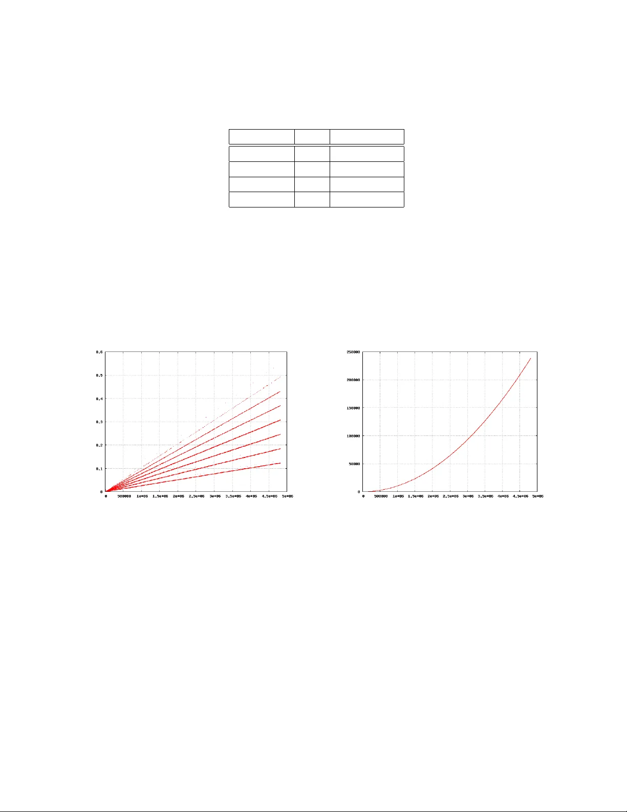
An Algorithm to Generate Square-F ree Num b ers and to Compute the M¨ obius F unction F. Auil auil@usp.br Abstract. W e in tro duce an algorithm that iterativ ely pro duces a sequence of nat- ural num b ers k i and functions b i defined in the in terv al [1 , + ∞ ). The n umber k i +1 arises as the first p oin t of discon tinuit y of b i ab o v e k i . W e derive a set of prop erties of b oth sequences, suggesting that (1) the algorithm produces square-free num b ers k i , (2) al l the square-free n umbers are generated as the output of the algorithm, and (3) the v alue of the M¨ obius function µ ( k i ) can b e ev aluated as b i ( k i +1 ) − b i ( k i ). The logical equiv alence of these properties is rigorously prov ed. The question remains op en if one of these prop erties can b e deriv ed from the definition of the algorithm. Numerical evidence, limited to 5 × 10 6 , seems to support this conjecture. Keyw ords: M¨ obius function, square-free num b ers, zeta function, Riemann h yp othesis. AMS Sub ject Classification: 11Y55, 11M99, 11Y35. 1 In tro duction A natural num b er n ∈ N is called squar e-fr e e , if the exp onen ts arising in its prime factor- ization n = p r 1 1 p r 2 2 · · · p r k k are all equal to 1, i.e., r 1 = r 2 = · · · = r k = 1. F or a natural n umber n with prime factorization as ab o v e, the M¨ obius function µ is defined as µ ( n ) =      1 if n = 1; ( − 1) P k i =1 r i , if n is square-free; 0 , otherwise. In other words, µ ( n ) is zero when n has a square factor, and otherwise giv es the parity of the num b er of (distinct) prime factors of n . The M¨ obius function has imp ortan t applica- tions in n umber theory , many of them concerning to the Riemann h yp othesis ab out the zeros of the zeta function, [1], [6], [7], [8]. 1 An outstanding problem in algorithmic num b er theory is to compute µ ( n ) efficiently without first factoring n . By “efficien tly” w e mean a n um b er of bit op erations b ounded b y a p olynomial in log n , the length of n in binary . As far as w e know, the question remains op en if the computation of µ ( n ) can b e done in p olynomial time, and in fact, nob o dy curren tly knows a w ay to compute it significantly faster than factoring n . In this pap er, w e presen t an algorithm that iteratively pro duces a sequence of num b ers k i and the v alue of µ ( k i ). In order to determine µ ( k i ), it is necessary to generate the whole sequence k 1 , k 2 , . . . , k i . Our algorithm is based on a sequence of arithmetical functions b i , with the n umbers k i arising as discon tinuit y p oin ts. These functions are closely related to the Nyman-Beurling approac h to the Riemann h yp othesis. The main result of the presen t pap er is a set of prop erties of the sequences k i and b i , suggesting that • The num b ers k i generated b y the algorithm are square-free. • The set of al l the square-free num b ers can b e generated by the algorithm. • The v alue of the M¨ obius function µ ( k i ) can b e ev aluated as b i ( k i +1 ) − b i ( k i ). W e are able to pro v e the logical equiv alence of these properties. Unfortunately , using the definition of the algorithm, w e cannot pro ve, neither disprov e, if one (then all) of these conditions are satisfied. Numerical evidence, limited to 5 × 10 6 , seems to supp ort the conjectures quoted ab o v e. This paper is organized as follo ws. The section 2 in tro duces the framework of the Nyman-Beurling approac h to Riemann h yp othesis. The section 3 provides the basic def- initions for this pap er, and the algorithm is defined in section 4. The main result of the presen t work is stated and prov ed in section 5, while further remarks are done in section 6. Finally , the implementation of the algorithm and numerical results are discussed in section 7. 2 Hilb ert Space Approac h to Riemann Hyp othesis Denote by b x c the intege r part of x , i.e., the greatest integer less than, or equal to, x . Define the fr actional p art function b y { x } = x − b x c . Given n ∈ N and tw o families of parameters { a k } n k =1 ⊂ C and { θ k } n k =1 ⊂ (0 , 1], we define a Beurling function as a function F n (the sub-index n included in the notation for con v enience) of the form F n ( x ) : = n X k =1 a k  θ k x  . (1) 2 F or a Beurling function F n , an elemen tary computation shows that Z 1 0 ( F n ( x ) + 1) x s − 1 dx = n X k =1 a k θ k s − 1 + 1 s 1 − ζ ( s ) n X k =1 a k θ s k ! ; (2) for the complex v ariable s ∈ C in the half-plane Re( s ) > 0, i.e. for s with p ositiv e real part. Here, ζ denotes the Riemann’s zeta function given by ζ ( s ) : = ∞ X k =1 1 k s . The classic references are [8] and [6]. A deriv ation of the relation (2) can b e found, for instance, in [2, p. 253]. It is useful (but not alwa ys necessary from a theoretical p oin t of view) to assume that the parameters defining the function F n satisfy the additional condition n X k =1 a k θ k = 0 . (3) In this case, the first term at the righ t-hand side of (2) v anishes, simplifying the expression. The iden tity (2) is the starting p oin t of the following theorem b y Beurling Theorem 1 (Beurling) . The zeta function ζ ( s ) has no zer os in the half-plane Re( s ) > 1 /p if and only if the set of (Beurling) functions { f θ ( x ) = { θ /x }} 0 <θ 6 1 is dense in L p ([0 , 1] , dx ) . See [2, p. 252] for a pro of of the Beurling theorem and further references. Note that for p = 2 this result provides an equiv alen t condition to the R iemann hyp othesis (RH) for the zeta function. This is the Beurling, or Nyman-Beurling, approac h to RH. The Beurling theorem ab ov e has an easy half part, whose pro of can b e sketc hed as follo ws. F rom relation (2) and assuming (3), we hav e      1 s 1 − ζ ( s ) n X k =1 a k θ s k !      =     Z 1 0 ( F n ( x ) + 1) x s − 1 dx     6 k F n ( x ) + 1 k   x s − 1   ; where the last relation follows using the Sch w arz inequality in L 2 ([0 , 1] , dx ). Therefore, if the first norm in the right-hand side ab o ve can b e done arbitrarily small for a suitable c hoice of n , a k ’s and θ k ’s, then the function ζ ( s ) could not ha ve zeros for Re( s ) > 1 / 2. W e will refer to the first condition abov e as the Beurling criterion (BC) for RH. Note also that in order to demonstrate the RH, it is sufficien t to prov e that the constant function equal to − 1 can b e arbitrarily approximated in the norm of the Hilbert space L 2 ([0 , 1] , dx ) by 3 Beurling functions F n of the form (1). It w as pro v ed in [4] that BC remains equiv alent to RH if the parameters θ k are restricted to b e recipro cal of natural n umbers, i.e. θ k = 1 /b k , with b k ∈ N . Sev eral appro ximating functions to − 1 of the form (1) were prop osed in the literature. F rom the relations (2) and (3), w e hav e that under the BC, the “partial sum” n X k =1 a k θ s k . (4) is an approximation to the recipro cal of the zeta function 1 /ζ ( s ), whic h is kno wn to ha v e an expression as a Diric hlet series 1 ζ ( s ) = n X k =1 µ ( k ) k s , (5) con vergen t for Re( s ) > 1. Therefore, a (naiv e) first choice for an approximating function w ould b e S n ( x ) : = n X k =1 µ ( k )  1 /k x  . (6) Note that this function do es not matches the condition (3). W e can handle this without subtlet y , just by subtracting the difference, that is given by g ( n ), where g ( t ) : = X N 3 k 6 t µ ( k ) k . (7) Therefore, a second c hoice would be B n ( x ) : = n X k =1 µ ( k )  1 /k x  − n g ( n )  1 /n x  (8) = n − 1 X k =1 µ ( k )  1 /k x  − n g ( n − 1)  1 /n x  . (9) Other v arian ts were also prop osed, as V n ( x ) : = n X k =1 µ ( k )  1 /k x  − g ( n )  1 x  . (10) Unfortunately , the sequences (6), (9) and (10) are kno wn to be not con vergen t to − 1 in L 2 ([0 , 1] , dx ), as prov ed in [3]. A survey on the Nyman-Beurling reform ulation of the Riemann h yp othesis and later dev elopments b y Baez-Duarte can b e found in [5]. 4 3 Basic Definitions In order to motiv ate the definitions b elow, assume that a Beurling function F n as in (1) is constan t b etw een the reciprocal of the natural n umbers. In other w ords, assume that suc h a function takes a constan t v alue in eac h of the in terv als ( 1 k +1 , 1 k ], for all k ∈ N (but the constan t v alue may differ from in terv al to interv al). In this case, the in tegral in (2) can b e expressed alternatively as an infinite series, in v olving the v alues of f n ( k ) : = F n (1 /k ). F urthermore, the v alues of F n ( x ) for all x ∈ [0 , 1] are completely determined b y the v alues of f n ( k ) for all k ∈ N . W e will call an arithmetic al Beurling function a function of the form f n ( k ) = F n (1 /k ), where F n is a Beurling function. W e in tro duce now, p erhaps the simplest, non-trivial, example of arithmetical Beurling function satisfying the condition (3). F or a, b ∈ N define the function β a,b as β a,b ( x ) : = n x a o − b a n x b o , (11) As the functions β a,b will b e the basic blo cks in our construction, w e summarize some of its elemen tary prop erties in the follo wing result. Lemma 1. Consider a, b ∈ R , with 0 < a < b . Then, a. n x a o and n x b o ar e right-c ontinuous, and line arly indep endent functions. b. β a,b ( x ) = 0 , when 0 6 x < a . c. L et k ∈ N b e such that ( k − 1) a < b 6 k a . Then, β a,b ( x ) = ( − j if j a 6 x < ( j + 1) a , for j = 1 , . . . , ( k − 2); − ( k − 1) if ( k − 1) a 6 x < b . d. Assume a, b ∈ N . Then, β a,b ( x ) is c onstant when k 6 x < k + 1 , for al l k ∈ N . Pr o of: (a): The right-con tin uit y is deriv ed from of b x c . Now, if c 1  x a  + c 2  x b  = 0 for all x , then for x = a w e hav e 0 = c 1  a a  + c 2  a b  = c 2 a b . Th us, c 2 = 0 and we hav e c 1  x a  = 0 for all x , and taking now x = a/ 2 w e get 0 = c 1  1 2  = c 1 / 2 and c 1 = 0. (b): If 0 6 x < a < b , then x/b < 1 and x/a < 1. Thus,  x a  − b a  x b  = x a − b a x b = 0. (c): Assume j = 1 , . . . , ( k − 2). Then, for j a 6 x < ( j + 1) a < b , we hav e x/b < 1 and j 6 x/a < ( j + 1). Th us,  x a  − b a  x b  = x a −  x a  − b a x b = x a − j − x a = − j . Analo- gously , for ( k − 1) a 6 x < b < k a , w e ha ve x/b < 1 and ( k − 1) 6 x/a < k . Thus, 5  x a  − b a  x b  = x a −  x a  − b a x b = x a − ( k − 1) − x a = − ( k − 1). (d): If x < b then (d) is true by (b) and (c) already prov en. Consider no w b 6 x . If k < x < k + 1 then x / ∈ N and th us x/a / ∈ N and x/b / ∈ N . Therefore, there exists k 0 and l 0 in N such that ak 0 < x < a ( k 0 + 1) and bl 0 < x < b ( l 0 + 1), and we hav e  x a  − b a  x b  = x a − k 0 − b a ( x b − l 0 ) = − k 0 + b a l 0 , which is a constant indep endent of x . As  x a  − b a  x b  is righ t-contin uous, by part (a), this is also true for k 6 x < k + 1. 4 The Algorithm W e will define a sequence of n umbers { k i } i ∈ N and functions { b i } i ∈ N iterativ ely as follo ws. Start with the follo wing definitions k 1 : = 1; k 2 : = 2; b 2 ( x ) : =  x k 1  − k 2 k 1  x k 2  . (12) Assuming no w that k i and b i are already defined, for i > 2 define iterativ ely k i +1 and b i +1 as follo ws. The num b er k i +1 is defined as k i +1 : = k i + j , where j is the least integer suc h that b i ( k i + j ) 6 = b i ( k i ). Once determined the num b er k i +1 , the function b i +1 is defined as b i +1 ( x ) : = b i ( x ) + (1 + b i ( k i ))  x k i  − k i +1 k i  x k i +1  . (13) Some elementary prop erties derived from these definitions are summarized in the follo wing result. Lemma 2. F or any i ∈ N we have a. b i is a right-c ontinuous function, which is c onstant b etwe en the natur al numb ers. b. b i +1 ( k i ) = − 1 . c. Assume k i +1 6 2 k i for i > 2 . Then, b i ( x ) = − 1 for al l x ∈ [1 , k i ) . In p articular, the se quenc e { b i } i ∈ N c onver ges p oint-wise to − 1 in [1 , + ∞ ) . 6 Pr o of: (a): Observ e that eac h b i is a (finite) linear com bination of β p,q . Therefore, this result is a direct consequence of Lemma 1. (b): Is an immediate consequence of definition (13). (c): F or induction on i . The case i = 2 is an immediate consequence of definition (12). Assume no w that b j ( x ) = − 1 when x ∈ [1 , k j ) for all j 6 i . If x < k i < k i +1 , then from definition (13) w e ha ve b i +1 ( x ) = b i ( x ) whic h is equal to − 1 b y the inductive h yp othesis. No w if k i 6 x < k i +1 6 2 k i , also from definition (13) w e ha ve b i +1 ( x ) = b i ( x ) + (1 + b i ( k i ))  x k i − 1 − k i +1 k i x k i +1  = b i ( x ) − 1 − b i ( k i ) = − 1 , b ecause b y the definition of k i +1 , the function b i ( x ) is constan t for x ∈ [ k i , k i +1 ). Remark: As b i is a constan t function b etw een the natural num b ers, the num b er k i +1 is the first p oin t of discon tin uity of b i ab o v e k i . 5 Main Result The next result is relev ant in order to establish a relationship b et w een the sequence { k i } i ∈ N , the v alues of µ ( k i ), and the square-free n umbers. Lemma 3. The fol lowing c onditions ar e e quivalent a. i X j =1 µ ( k j ) k j = 1 + b i ( k i ) k i , for i > 2 . b. b i ( x ) = i − 1 X j =1 µ ( k j )  x k j  − k i i − 1 X j =1 µ ( k j ) k j !  x k i  , for i > 2 . c. µ ( k i ) k i = 1 + b i ( k i ) k i − 1 + b i − 1 ( k i − 1 ) k i − 1 , for i > 3 . F urthermor e, if the c ondition k i +1 < 2 k i is valid for i > 2 , then al l c onditions ab ove ar e also e quivalent to the fol lowing ones d. µ ( k i +1 ) = b i ( k i +1 ) − b i ( k i ) , for i > 2 . e. i X j =1 µ ( k j )  k i k j  = 1 , for i > 1 . 7 Pr o of: In order to prov e the logical equiv alence betw een all conditions in Lemma 3, we separately will prov e, first of all, the equiv alences (a) ⇔ (b) and (a) ⇔ (c). Then, after the in tro duction of the additional condition k i +1 < 2 k i , we will pro ve the equiv alence b etw een (d) ⇔ (c) and (e) ⇔ (b). (a) ⇒ (b): F or induction on i . F or i = 2, from definition (12) w e hav e b 2 ( x ) =  x k 1  − k 2 k 1  x k 2  = µ ( k 1 )  x k 1  − k 2 µ ( k 1 ) k 1  x k 2  . (14) Assuming no w that condition (b) follows for all j such that j 6 i , we hav e b i +1 ( x ) = b i ( x ) + (1 + b i ( k i ))  x k i  − k i +1 k i  x k i +1  = i − 1 X j =1 µ ( k j )  x k j  − k i i − 1 X j =1 µ ( k j ) k j !  x k i  + (1 + b i ( k i ))  x k i  − k i +1 k i  x k i +1  = i − 1 X j =1 µ ( k j )  x k j  − k i i − 1 X j =1 µ ( k j ) k j !  x k i  + k i i X j =1 µ ( k j ) k j !  x k i  − k i +1 k i  x k i +1  = i − 1 X j =1 µ ( k j )  x k j  − k i i − 1 X j =1 µ ( k j ) k j !  x k i  + k i i X j =1 µ ( k j ) k j !  x k i  − k i +1 i X j =1 µ ( k j ) k j !  x k i +1  = i − 1 X j =1 µ ( k j )  x k j  + k i µ ( k i ) k i  x k i  − k i +1 i X j =1 µ ( k j ) k j !  x k i +1  = i X j =1 µ ( k j )  x k j  − k i +1 i X j =1 µ ( k j ) k j !  x k i +1  ; (15) and this prov es condition (b) for i + 1. Here, in the first equality we hav e used the induc- tiv e hypothesis and in the second one we ha ve used condition (a). 8 (b) ⇒ (a): F rom Lemma 2 (b), b y condition (b) we hav e 0 = 1 + b i +1 ( k i ) = 1 + i X j =1 µ ( k j )  k i k j  − k i +1 i X j =1 µ ( k j ) k j !  k i k i +1  = 1 + i − 1 X j =1 µ ( k j )  k i k j  + µ ( k i )  k i k i  − k i +1 i X j =1 µ ( k j ) k j ! k i k i +1 = 1 + i − 1 X j =1 µ ( k j )  k i k j  − k i i X j =1 µ ( k j ) k j ! = 1 + b i ( k i ) − k i i X j =1 µ ( k j ) k j ! ; (16) and this prov es condition (a). Here w e ha v e used that n k i k i +1 o = k i k i +1 , (b ecause k i k i +1 < 1), that n k i k i o = 0, and also the relation b i ( k i ) = P i − 1 j =1 µ ( k j ) n k i k j o , which is an easy conse- quence of condition (b). (a) ⇒ (c): Using condition (a) for i and i − 1 we hav e i X j =1 µ ( k j ) k j = 1 + b i ( k i ) k i , (17) i − 1 X j =1 µ ( k j ) k j = 1 + b i − 1 ( k i − 1 ) k i − 1 ; (18) and subtracting (18) from (17) w e get condition (c). (c) ⇒ (a): Denoting α ( i ) : = 1+ b i ( k i ) k i , from (c) w e hav e i X j =1 µ ( k j ) k j = µ ( k 1 ) k 1 + µ ( k 2 ) k 2 + i X j =3 α ( j ) − α ( j − 1) = 1 − 1 2 + α ( i ) − α (2) = 1 − 1 2 + α ( i ) − 1 + b 2 ( k 2 ) k 2 = 1 − 1 2 + α ( i ) − 1 2 = α ( i ) = 1 + b i ( k i ) k i . (19) Here w e hav e used that b 2 ( k 2 ) = 0, by definition (12). Therefore, w e hav e prov ed (b) ⇔ (a) ⇔ (c). Assume no w condition k i +1 < 2 k i , for i > 2. 9 (d) ⇔ (c): F rom definition (13) we ha ve b i ( k i ) = b i − 1 ( k i ) + (1 + b i − 1 ( k i − 1 ))  k i k i − 1  − k i k i − 1  k i k i  = b i − 1 ( k i ) + (1 + b i − 1 ( k i − 1 ))  k i k i − 1  = b i − 1 ( k i ) + (1 + b i − 1 ( k i − 1 ))  k i k i − 1 −  k i k i − 1  = b i − 1 ( k i ) + (1 + b i − 1 ( k i − 1 ))  k i k i − 1 − 1  = b i − 1 ( k i ) + (1 + b i − 1 ( k i − 1 )) k i k i − 1 − (1 + b i − 1 ( k i − 1 )) . (20) Observ e that the additional condition implies 1 < k i k i − 1 < 2, and therefore j k i k i − 1 k = 1. F rom (20) follo ws 1 + b i ( k i ) k i − 1 + b i − 1 ( k i − 1 ) k i − 1 = b i − 1 ( k i ) − b i − 1 ( k i − 1 ) k i , (21) for i 6 3. The equiv alence b etw een (d) and (c) is a direct consequence of (21) ab ov e. (b) ⇒ (e): F rom Lemma 2 (b), b y condition (b) we hav e 0 = 1 + b i ( k i − 1 ) = 1 + i − 1 X j =1 µ ( k j )  k i − 1 k j  − k i i − 1 X j =1 µ ( k j ) k j !  k i − 1 k i  = 1 + i − 1 X j =1 µ ( k j ) k j ! k i − 1 − i − 1 X j =1 µ ( k j )  k i − 1 k j  − k i i − 1 X j =1 µ ( k j ) k j ! k i − 1 k i + k i i − 1 X j =1 µ ( k j ) k j !  k i − 1 k i  = 1 − i − 1 X j =1 µ ( k j )  k i − 1 k j  , (22) and this prov es condition (e). Here, w e hav e used that k i − 1 k i < 1 and therefore j k i − 1 k i k = 0. (e) ⇒ (b): Assume condition (e) v alid for all i ∈ N . W e will pro ve (b) by induction on i . Condition (b) for i = 2 follo ws from definition (12) as done in the pro of (a) ⇒ (b) ab ov e. Assume now condition (b) v alid for all n 6 i . Using the notation g ( i ) = P i j =1 µ ( k i ) k i , w e 10 ha ve b i ( k i +1 ) = i − 1 X j =1 µ ( k j )  k i +1 k j  − k i i − 1 X j =1 µ ( k j ) k j !  k i +1 k i  = k i +1 g ( i − 1) − i − 1 X j =1 µ ( k j )  k i +1 k j  − k i g ( i − 1) k i +1 k i + k i g ( i − 1)  k i +1 k i  = − i − 1 X j =1 µ ( k j )  k i +1 k j  + k i g ( i − 1) = −  1 − µ ( k i +1 )  k i +1 k i +1  − µ ( k i )  k i +1 k i  + k i g ( i − 1) = − (1 − µ ( k i +1 ) − µ ( k i )) + k i g ( i − 1) = k i g ( i − 1) + µ ( k i +1 ) + µ ( k i ) − 1 . (23) Here w e ha v e used j k i +1 k i k = 1 (a consequence of the additional condition) and (e). Anal- ogously w e hav e b i ( k i ) = i − 1 X j =1 µ ( k j )  k i k j  − k i i − 1 X j =1 µ ( k j ) k j !  k i k i  = i − 1 X j =1 µ ( k j )  k i k j  = k i g ( i − 1) − i − 1 X j =1 µ ( k j )  k i k j  = k i g ( i − 1) −  1 − µ ( k i )  k i k i  = k i g ( i − 1) − (1 − µ ( k i )) = k i g ( i − 1) + µ ( k i ) − 1 . (24) No w, subtracting (24) from (23) we get condition (d). But we ha v e already prov ed that (d) ⇒ (c) ⇒ (a) ⇒ (b). 6 Discussion The definitions in section 4 provide an algorithm to pro duce iteratively a sequence of n umbers { k i } i ∈ N and functions { b i } i ∈ N . The Lemma 3 in section 5 states a circle of logi- cally equiv alen t prop erties of b oth sequences. 11 The condition (b) of Lemma 3 suggests that the functions b i are the arithmetical coun- terpart of the approximating functions B n in the relation (9). Ho wev er, note that our definition of b i in section 4 is quite differen t of B n . The condition (d) of Lemma 3 is related with the conjecture that the algorithm pro- duces square-free num b ers k i , and also provides the v alue of the M¨ obius function µ ( k i ). Note that the v alue of b i ( k i +1 ) − b i ( k i ) is nev er zero, b y the definition of the algorithm in section 4. The condition (e) of Lemma 3 is related with the conjecture that the algorithm pro- duces al l the square-free n umbers. Indeed, if condition (e) w ere true, this w ould b e a corollary of a w ell known result; see [1, p. 66]. The condition k i +1 < 2 k i in Lemma 3, sufficient for (d) and (e), seems to b e also necessary , as the following heuristic argumen t suggests. It is kno wn that the square-free n umbers are distributed in N with densit y 6 /π 2 ; see [7, Thm. 333, p. 269]. Therefore, we can estimate the av erage distance betw een tw o consecutive square-free n umbers as π 2 / 6. Consequen tly , k i +1 ≈ k i + π 2 / 6, or k i +1 /k i ≈ 1 + π 2 / 6 k i . The last expression is less than 2 for k i > π 2 / 6 ≈ 1 . 64. Thus, condition k i +1 < 2 k i for i > 2 seems to b e reasonable also. Unfortunately , using the definition of the algorithm giv en in section 4, we cannot pro ve, neither dispro ve, if one of the conditions in Lemma 3 are satisfied. Note also that the algorithm cannot compute isolated v alues of µ ( k i ). In order to determine µ ( k i ), it is necessary to generate the whole sequence k 1 , k 2 , . . . , k i . 7 Numerical Results The algorithm defined in section 4 was implemen ted using the Jav a programming lan- guage. The source co de can b e downloaded from http://143.107.59.106:9620/camille/ beurling.tar.bz2 . This archiv e pro vides, in fact, t w o slightly different implemen tations of the algorithm. 7.1 The class Beurling The metho ds in this class compute the sequences k i and b i , storing the v alues in an arra y with fixed size. The main metho d takes a natural num b er n as input. Its output is a file con taining 3-uplas ( k i , µ ( k i ) , t i ), for i from 3 to n . Here, t i is the running time, in seconds, b et w een the computation of µ ( k i − 1 ) and µ ( k i ). The v alues of the M¨ obius function are calculated using the identit y in Lemma 3 (d). The main metho d in this class also verifies: 12 • If each one of the num b ers k i is square-free. • If there exist even tually square-free num b ers b etw een k i and k i +1 that are not gen- erated b y the algorithm. • The condition k i +1 < 2 k i , equiv alen t to the gap k i +1 − k i < k i . These additional v erifications are not included in the running time t i . Running this class with n = 1 × 10 6 , the size of the output file was ab out 10 MB. T o estimate the running time, w e generate a graphic with the pairs ( k i , t i ); see figure 1. Figure 1: P airs ( k i , t i ), where t i is the running time (seconds) b etw een the com- putation of µ ( k i − 1 ) and µ ( k i ), using the class Beurling . Figure 2: Pairs ( k i , T i ), where T i is the total running time (seconds) for the com- putation of µ ( k i ), using the Ja v a class Beurling . This graphic seems to suggest that square-free n umbers can b e divided in classes, and for eac h of these classes, the running time starting from the previous iteration t i is con- stan t. W e v erify that all the square-free n umbers in the range analyzed are generated b y the program, and satisfy the condition k i +1 < 2 k i , for i > 2. T o estimate the total running time T i to compute µ ( k i ), we use the formula T i = P i k =1 t k . The graphic with the pairs ( k i , T i ) is sho wn in figure 2. The program produced also four squar e-ful l , i.e. non square-free, n umbers, shown in the table 1. All these square-full n umbers k i satisfy b i ( k i +1 ) − b i ( k i ) = µ ( k i ) = 0. Ho wev er, as already stated, b y the definition of the algorithm in section 4, it must b e b i ( k i +1 ) − b i ( k i ) 6 = 0 for any generated num b er. Therefore, w e strongly b eliev e that the square-full n umbers are generated purely by rounding errors. 13 Num b er k µ ( k ) Divisible by 440375 0 5 2 551208 0 2 2 799460 0 2 2 979275 0 5 2 T able 1: The four square-full num b ers pro duced b y the class Beurling , with n = 1 × 10 6 . 7.2 The class BeurlingArrayList This class w orks as the previous one, but the computed v alues are stored in an arra y with dynamic size. W e use this class to pro cess n = 5 × 10 6 n umbers, using a relatively mo dest desktop mac hine. The graphics with the pairs ( k i , t i ) and ( k i , T i ) are sho wn in figures 3 and 4, resp ectiv ely . Figure 3: P airs ( k i , t i ), where t i is the running time (seconds) b etw een the com- putation of µ ( k i − 1 ) and µ ( k i ), using the class BeurlingArrayList . Figure 4: P airs ( k i , T i ), where T i is the total running time (seconds) for the computation of µ ( k i ), using the class BeurlingArrayList . As in the case of figure 1, the square-free num b ers k i seems to b e divided in classes. Ho wev er, in this case, the running time b et w een t wo successiv e iterations t i gro ws linearly with k i . All the square-free num b ers in the range analyzed are generated by the program, and satisfy the condition k i +1 < 2 k i , for i > 2. In the range analized, tw en ty square-full n umbers w ere also generated b y this class, probably b y rounding errors, as explained ab o v e. 14 8 Concluding Remarks In section 4 we define an algorithm that iterativ ely pro duces a sequence of num b ers k i and functions b i . The lemma 3 states a set of prop erties of these sequences suggesting that • The num b ers k i generated b y the algorithm are square-free. • The set of al l the square-free num b ers can b e generated by the algorithm. • The v alue of the M¨ obius function µ ( k i ) can b e ev aluated as µ ( k i ) = b i ( k i +1 ) − b i ( k i ). In section 5 we prov e the logical equiv alence of these prop erties. Unfortunately , using the definition of the algorithm, w e cannot prov e, neither dispro v e, if one of these conditions are satisfied. Note also that in order to determine µ ( k i ), it is necessary to generate the whole sequence k 1 , k 2 , . . . , k i . Numerical evidence seems to support the conjectures quoted ab ov e. How ev er, this evidence is limited, and certainly not conclusiv e. References [1] T. M. Ap ostol, Intr o duction to Analytic Numb er The ory , Springer-V erlag, New Y ork, 1976. 1, 6 [2] W. F. Donogh ue, Distributions and F ourier T r ansforms , Academic Press, New Y ork, 1969. 2, 2 [3] L. B´ aez-Duarte, Arithmetic al Asp e cts of Beurling’s R e al V ariable R eformulation of the Riemann Hyp othesis . arXiv:math/0011254v1 [math.NT]. Av ailable in http:// arxiv.org/abs/math/0011254v1 . 2 [4] L. B´ aez-Duarte, A Str engthening of the Nyman-Beurling Criterion for the Rie- mann Hyp othesis . Atti Acad. Naz. Lincei 14 (2003) 5-11. arXiv:math/0202141v2 [math.NT]. Av ailable in . 2 [5] B. Bagchi, On Nyman, Beurling and Baez-Duarte’s r eformulation of the Riemann hyp othesis , Pro c. Indian Acad. Sci. (Math. Sci) 116 No. 2 (2003) 137-146. 2 [6] H. M. Edwards, R iemann ’s Zeta F unction , Academic Press, New Y ork, 1974. 1, 2 [7] G. H. Hardy , E. M. W right. A n Intr o duction to the The ory of Numb ers , Oxford Univ ersity Press, 5th ed., 1980. 1, 6 15 [8] E. C. Titc hmarsh, The the ory of the Riemann zeta function , Oxford Univ. Press, Oxford, 1951. 1, 2 F ernando Auil Escola de Artes, Ci ˆ encias e Humanidades Univ ersidade de S˜ ao Paulo Arlindo Bettio 1000 CEP 03828-000 S˜ ao Paulo - SP Brasil E-mail: auil@usp.br 16