Posterior model probabilities computed from model-specific Gibbs output

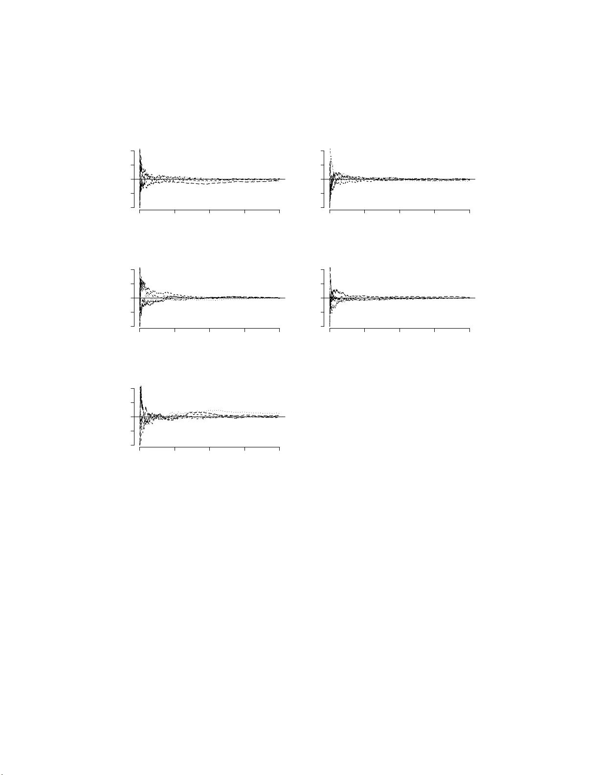
P osterior Mo del Probabilities Computed F rom Mo del-Sp ecific Gibbs Output Ric hard J. Bar k er ∗ and Willi am A. Link † Octob er 2 3, 201 8 Rev ersible jump Mark ov c hain Monte Carlo (RJMCMC) extends ordinary MCMC metho ds for use in Bay esian m ultimo del inference. W e show that RJMCMC can b e implemen ted as Gibbs sampling with alternating up dates of a mo del indicator and a v ector-v alued “palette” of parameters denoted ψ . Lik e an artist uses the palette to mix dabs of color fo r sp ecific needs, w e create mo del-sp ecific parameters f r o m the set av aila ble in ψ . This descrip- tion not only remov es some o f the my stery of R JMCMC, but also pro vides a basis f o r fitting mo dels one at a time using ordinary MCMC and computing mo del we igh ts or Bay es factors by p ost-pro cessing the Mon te Carlo output. ∗ Department of Mathematics and Statistics, Universit y of O tago, P .O. B ox 56 Dunedin, New Zea land † Patuxen t Wildlife Research Center, Laurel, MD 2 0708, USA 1 W e illustrate our pro cedure using sev eral examples . KEY W O R DS: Rev ersible jump Mark ov c ha in Mon te Carlo, Bay esian m ul- timo del inference, Bay es factors, Poste rior mo del pro babilities. 1 In tro duct i on A natural Bay esian approach to pro blems of m ultimo del inference is to com- pute p osterior mo del probabilities, or equiv alently Ba y es factors, given priors and data. Ba y es factors in v olve marginal lik eliho o ds and can b e difficult to calculate. Here w e address the problem of estimating p osterior mo del proba- bilities, and pro vide a represen ta tion of rev ersible jump Mark o v c hain Mon te Carlo (RJMCM C) that allo ws us to use MCMC o ut put obtained fitting mo d- els one at a time. T ec hniques ha v e been prop osed for computing Bay es factors using MCMC output from indep enden t c hains generated for differen t mo dels (f o r example, Chib 1995) or b y using a searc h ov er the join t space of mo del indicators M ∈ M and mo del parameters θ j ∈ Θ j giv en by M × Q j ∈M Θ j . Either approac h is difficult in practice and it is common for mo del selection to b e based instead on a deviance information criterion (D IC) (Spiegelhalter et al. 2002). How ev er, there is no theoretical justification for using DIC to pro duce mo del w eigh ts or Ba yes factors. 2 Rev ersible jump Mark o v c ha in Mon te Carlo is an extension of o rdinary MCMC, for m ultimo del inference. In this broader context, the p osterior dis- tribution under in v estigation describ es par ameters for a collection of mo dels, rather than a single mo del; furthermore the p o sterior distribution describ es mo del uncertain t y through we igh ts on a categorical v ar ia ble w e call Mo d el . A k ey step in implemen ting RJMCMC is the specification of bijections de- scribing relationships b etw een the parameters of v arious mo dels (e.g., G reen 1995; Gelman et al. 20 04). RJMCMC is usually describ ed in terms of  K 2  suc h bijections where K is the n um b er of mo dels in the mo del set M . Link and Bark er (2010) outlined an alternative form ula t ion of RJMCMC as simple Gibbs sampling, alternating b et w een up dating a palette of parameters ψ , whic h is of the same dimension for all models, a nd the categorical v ariable Mo del . There are K bijections, one relating eac h mo del’s parameters to the palette ψ ; the  K 2  bijections typic ally describ ed are obtained fro m these. Careful construction of the palette and K bijections allo ws RJMCMC to be carried out using samples from mo del-sp ecific p osteriors, obtained one mo del at a time. Here we illustrate this approac h and extend Link and Barker (2010) b y showing that mov es b et w een mo dels can b e written so that they in v olve a direct draw from a kno wn categorical distribution with all mo dels in the sample space . This formulation ob viates the need for use o f a Metrop olis- Hastings step that only allow s pair-wise comparison of mo dels and can b e easier to implemen t than RJMCMC in its usual incarnations. 3 2 A d escripti on of RJMCMC Supp ose that w e wish to ev aluate the relative suppo rt provided b y data y to mo dels M k , k = 1 , 2 , . . . , K , these mo dels b eing fully know n except for parameter v ectors θ ( k ) for whic h w e ha ve specified priors. RJMCMC can b e expressed as simple Gibbs sampling, with dra ws alter- nating betw een the categorical v ariable Mo del a nd a univ ersal vec tor-v alued parameter ψ . W e compare ψ to an ar tist’s palette: as the artist com bines colors on her palette to pro duce colors needed for sp ecific a pplications, so comp onen ts of ψ are combined to pro duce mo del-specific parameters θ ( k ) . The impo rtan t feature of RJMCMC is that the en tire palette ψ is updat ed at each step of the Gibbs sampler (rather than simply those comp onen ts relating to the presen t mo del). F ollow ing Link and Bark er (2010) the palette of parameters ψ is a v ector of dimension d greater than or equal to t he dimension of the most com- plex mo del in the mo del set. P ara meter v ector θ ( k ) can b e reco v ered fro m the palette ψ b y means of a known (in v ertible) mapping g k ( ψ ) = Θ ( k ) = ( θ ( k ) , u ( k ) ) ′ . V ector u ( k ) is irr elev ant to mo del M k , serving only to matc h the dimension of Θ ( k ) and ψ , so that g k ( · ) can b e defined as a bijection. Th us if mo del M 2 has parameter space of dimension 7 , and d = 10, v ector u (2) will ha v e dimension 3. Note that the  K 2  bijections typically required for RJMCMC are induced b y our K bijections b et w een the palette and mo del-sp ecific parameter spaces: 4 for mo dels M j and M k w e hav e g j k ( Θ ( j ) ) ≡ g k ◦ g − 1 j ( Θ ( j ) ) = g k ( ψ ) = Θ ( k ) . W e m ust sp ecify a prior for ψ and in doing so accommo da te mo del sp ecific priors [ θ ( k ) | M odel = M k ], whic h for simplicit y we write a s [ θ ( k ) | M k ]. W e hav e [ Θ ( k ) | M k ] = [ θ ( k ) , u ( k ) | M k ] = [ θ ( k ) | M k ] [ u ( k ) | θ ( k ) , M k ] . All that is needed is a sp ecification of [ u ( k ) | θ ( k ) , M k ]; given that u ( k ) has no role in inference, it will b e con v enien t to assume it is conditiona lly indep en- den t of θ ( k ) , so that [ u ( k ) | θ ( k ) , M k ] = [ u ( k ) | M k ]. The sp ecific c hoice do es not mat ter, except fo r tuning the RJMCMC alg orithm. F rom [ Θ ( k ) | M k ] w e obta in [ ψ | M k ] using the c ha ng e of v ariables theorem in terms o f a prio r f k ( Θ ( k ) ) = [ θ ( k ) , u ( k ) | M k ]. The prior on ψ is then [ ψ ] = X k [ ψ | M k ][ M k ] where [ ψ | M k ] = f k ( g k ( ψ ))     ∂ g k ( ψ ) ∂ ψ     . (1) Under this formu lation, Gibbs sampling consists of cyclical sampling of full conditional distributions, alternating b et w een draws from [ ψ | M k , y ] to up date ψ , and f rom [ { M 1 , . . . , M K }| ψ , y ] to up date Mo del . 5 Up dating ψ T o dra w from the full conditional [ ψ | M k , y ] it suffices to dra w from [ θ ( k ) | M k , y ] and [ u ( k ) | M k ] and then to apply the in vers e transformation g − 1 k ( Θ ( k ) ) to ob- tain a dra w for ψ . The dra w from [ θ ( k ) | M k , y ] can either b e made directly , if the distribution is of con v enien t for m, or b y simulation. Another po ssibilit y , often an a t trac- tiv e alternative , is to take a random draw from the stored MCMC output of an earlier analysis of mo del M k . Up dating the mo del The full-conditional for Mo del is categor ical with probabilities: Pr( M k | · ) = [ y | ψ , M k ][ ψ | M k ][ M k ] P j [ y | ψ , M j ][ ψ | M j ][ M j ] , for k = 1 , . . . , K . If w e a r e willing to calculate all of these probabilities, w e can up date Mo del by a direct draw from this f ull-conditional distribution. Chain means of mo del indicato rs I ( M odel = M k ) con v erge to the full condi- tional mo del probabilities, but greater efficiency is a v ailable b y using c hain means o f the full conditional mo del probabilities, whic h also conv erge to the p osterior mo del probabilities. As an alternativ e, w e can up dat e mo del indicators b y a Metrop o lis- Hastings step if the mo del candidate generator only allo ws limited transitions, for example, to a near neigh b or in a graphical mo del sense. The adv antage 6 of this approac h is that w e compute a smaller set of categorical pr o babilities, corresp onding to the neighborho o d set. In this case w e m ust compute p o s- terior mo del probabilities by c hain means of indicators I ( M o del = M k ). Expressing RJMCMC as simple G ibbs sampling provides the key innov a- tion of our fo rm ula tion: it allo ws us to fit mo dels one at a time using ordinary MCMC and then compute mo del w eights or Ba y es fa ctors b y p ost-pro cessing the Mon te Carlo output. Th us, w e hav e a simple 2-stage pro cedure that can b e used for computing mo del pr o babilities: Stage 1: P ro duce samples of [ ψ | y , M k ] for eac h k . Begin b y sampling [ θ ( k ) | y , M k ]. This can b e a ccomplished b y running a n MCMC sampler fo r M k , pro cessing it in the usual wa y , discarding a n y ini- tial burn-in iterations, and storing the results. (In cases where the p osterior distribution for θ ( k ) is of a kno wn and easily sampled form, w e do so.) F or eac h sampled v alue θ ( k ) , inde p enden t ly sample an auxiliary v ariable u ( k ) from [ u ( k ) | M k ] and calculate ψ = g − 1 k (( θ ( k ) , u ( k ) ) ′ ). The collection of sampled v al- ues ψ is a sample of [ ψ | y , M k ]. Stage 2: Post-pro cess the mo del sp ecific outputs. P o sterior mo del probabilities can b e computed in one of t wo w a ys. The first metho d is based on generating a Marko v chain of the categorical v ariable 7 Mo del that can b e used a s a p osterior sample from [ M o del | y ]. The second metho d is based on generating a Marko v c hain of b etw een-mo del transition probabilities that can b e used to estimate t he b etw een-mo del transition ma- trix. The steady state marginal distribution of this matrix corresp onds to the p osterior mo del probabilities. Metho d 1 A p osterior sample Mo del (1) , Mo del (2) , . . . , Mo del ( j ) , . . . can b e generated as follows : (a) Initialize Mo d el , sa y with M od el (1) = M 1 . (b) Iterate fr o m j = 1 to some large num b er J , and at eac h step: (i) If Mo del ( j ) = M k , draw a v alue ψ ( j ) from the stored sample of [ ψ | y , M k ] from Stage 1. (ii) Compute π ( j ) k = Pr( M odel = M k | ψ ( j ) , y ), for each k . This calcu- lation requires the Jacobian of the transformation Θ ( k ) = g k ( ψ ) as in eq. (1), ev aluated a t ψ ( j ) . (iii) Sample Mo del ( j +1) from a categorical distribution with sample space { M 1 , M 2 , . . . , M K } and probabilit y v ector π ( j ) =  π ( j ) 1 , π ( j ) 2 , . . . , π ( j ) K  ′ . The relative frequency with whic h M odel ( j ) = M k appro ximates the p oste- rior mo del proba bility for M k . A b etter estimate (Rao-Blackw ellized) is the c ha in mean of v a lues π ( j ) k . 8 Metho d 2 A further impro v emen t on this appro ximation can b e made b y mar g inalizing at stage 1, ob viating the need for the construction of a Mark ov c hain of mo del indicators in the second stage. F or eac h mo del w e can compute Pr( M k | ψ , M h ) forming a Marko v chain o f transition probabili- ties f rom mo del h to mo del k ( h, k ∈ 1 , . . . , K ). These can then b e a v era g ed to form an a pproximation to the sto chastic matrix gov erning mo del-to - mo del transitions. Giv en an estimate of this tra nsition matrix we can obtain corre- sp onding estimates of the p osterior mo del probabilities as the limiting distri- bution obtainable b y normalizing the left eigen v ector of the transition matrix asso ciated with the eigen v alue 1.0 (Seb er 2 008). 3 Examples 3.1 Radiata pine data Carlin and Chib (1995), Han and Carlin (20 01), a nd man y others a nalyze data take n fro m Williams (1 959). The resp onse v ariable y i is the maxim um compressiv e strength parallel to the grain fo r 42 radiata pine b oards. Two explanatory v ariables are considered: the first is the sp ecimen’s densit y , x i , and the second is the sp ecimen’s densit y ha ving adjusted f or resin conten t, z i . Resin increases the densit y of b oards without increasing their compress iv e 9 strength. Carlin and Chib (199 5) considered t w o mo dels: Mo del 1: y i = α + β ( x i − ¯ x ) + ε i , ε i ∼ N (0 , σ 2 x ) and Mo del 2: y i = γ + δ ( z i − ¯ z ) + ε i , ε i ∼ N (0 , σ 2 z ) . In b oth cases the error s ε are a ssumed iid among observ ations, conditional on the parameters. As priors, Carlin and Chib (1995) used N (( 3 000 , 185) ′ , diag(1 0 6 , 10 4 )) pri- ors on ( α, β ) ′ and ( γ , δ ) ′ , and inv erse gamma priors on σ 2 x and σ 2 z , b oth ha ving mean a nd standard deviation equal to 300 2 . This quirky choice of priors w as made to b e v ague but with exp ectations corresp onding roughly to the pa- rameter estimates obtained by fitting t he mo del b y least squares. W e fitted eac h of these mo dels indep enden tly using BUGS (Lunn et al. 2000) and the ab o v e priors, running three c hains of 60,000 eac h with distinct starting v alues. D iscarding the first 10,000 of eac h c hain as a burn- in left us with a p osterior sample of 1 5 0,000 for θ (1) and θ (2) . W e co ded a rev ersible jump algorithm in whic h g 1 ( ψ ) = ( α, β , σ 2 x ) ′ and g 2 ( ψ ) = ( γ , δ, σ 2 z ) ′ . In this case, [ ψ | M 1 ] = [ ψ | M 2 ], and the mo del up date is based on t he relativ e v alues 10 of the lik eliho o ds w eigh ted b y the mo del prior s Pr( M k ): Pr( M k | y , ψ ) = Pr( M k ) e − 1 2 ψ 3 P 42 i =1 ( y i − µ ik ) 2 Pr( M 1 ) e − 1 2 ψ 3 P 42 i =1 ( y i − µ i 1 ) 2 + Pr( M 2 ) e − 1 2 ψ 3 P 42 i =1 ( y i − µ i 2 ) 2 , where µ ik =      ψ 1 + ψ 2 ( x i − ¯ x ) k = 1 ψ 1 + ψ 2 ( z i − ¯ z ) k = 2 . F ollow ing Han and Carlin (2001) we assigned mo del prio r s of Pr( M 1 ) = 0 . 9995 and Pr( M 2 ) = 0 . 0005 to ensure that t he t w o mo dels w ere visited in roughly equal prop o rtion. Starting at mo del 1 or model 2 the chain fo r the p osterior model probabilit y conv erges rapidly (Figur e 1). Aft er running the t w o c hains for 20 0,000 iterations a nd discarding the first 100 ,0 00 as a burn- in, our estimate of the p osterior mo del probabilit y w as 0.709 correspo nding to a Ba y es factor B F 21 of 4870 . These are in close agreemen t with the exact v alues o f Pr( M 2 | y ) = 0 . 70865 and B F 21 = 486 2 rep orted b y Han a nd Carlin (2001). Figure 1 ab out here Using our second metho d, w e sampled 200,000 v alues of ψ from each c ha in h , and for the i th sample w e calculated Pr( M k | ψ ( i ) , M h ) ( k = 1 , 2). Av eraging across i w e obtain an estimated transition matrix of :    0 . 6003 0 . 3997 0 . 1651 0 . 8349    11 with steady-state marg ina l distribution of (0 . 2924 , 0 . 7076) ′ , corresp onding to B F 21 = 483 8. 3.2 T rout return rates Link and Bark er (200 6) rep o rt an a nalysis based on fitting logistic regression mo dels to the return rates fo r bro wn trout expressed in terms of sex S i and length L i effects. Mo deling the return indicator y i ∼ B er n ( p i ) they considered fiv e mo dels: 1. η i = β 0 2. η i = β 0 + β 1 S i 3. η i = β 0 + β 2 L i 4. η i = β 0 + β 1 S i + β 2 L i 5. η i = β 0 + β 1 S i + β 2 L i + β 3 S i L i where η i = logit( p i ). Link and Bark er (2006) used the fo llo wing priors on parameters: [ β k | V , M k ] =                        N (0 , V − 1 ) k = 1 N (0 , (2 V ) − 1 ) k = 2 N (0 , (2 V ) − 1 ) k = 3 N (0 , (3 V ) − 1 ) k = 4 N (0 , (4 V ) − 1 ) k = 5 12 where V has a Ga (3 . 29 , 7 . 8 0) prior distribution. This c hoice w as motiv ated b y the observ ation tha t if lo git( p ) ∼ N (0 , V − 1 ) and V ∼ Γ(3 . 29 , 7 . 80) , then the marginal distribution o f p is v ery nearly uniform on [0,1]. With S i and L i ha ving b een standardized, these choices of priors ensure that the prior on e η i / (1 − e η i ) = p i is appro ximately U (0 , 1 ) for S i = ± 1 and L i ± 1. P alette and bijections Eac h elemen t of ψ is directly asso ciated with either an elemen t o f the beta v ector or with a supplemen ta l v ariable u (T able 1): The parameter V is part Mo del ψ 1 2 3 4 5 ψ 1 β 0 β 0 β 0 β 0 β 0 ψ 2 u 1 β 1 u 1 β 1 β 1 ψ 3 u 2 u 1 β 2 β 2 β 2 ψ 4 u 3 u 2 u 2 u 1 β 12 T a ble 1: Association b et w een elemen ts of ψ and elemen ts o f β k , sp ecific parameters for mo del M k and suppleme n tal v ariables u k used in mo del M k for matc hing the parameter dimension t o ψ . of the prior sp ecification and is common to all mo dels so w e c hose to lea ve it out of the palette sp ecification, althoug h this is not necessary . Up dates for V were stored when eac h mo del was fitted. F or a particular mo del, the priors on the supplemen tal v ariables w ere the same as the prio r s used fo r the β co efficien ts in that mo del, and in eac h case the Jacobian of the t r ansformation from θ ( k ) to ψ is an iden tit y matrix of dimension 5. 13 As a n example, Mo del 1 (constan t only) has parameter v ector θ (1) = β 0 with supplemen tal v ariables u (1) = ( u 1 , u 2 , u 3 ) ′ . Th us g 1 ( ψ ) = g 1       ψ 1 . . . ψ 4       = Θ (1) =          β 0 u 1 u 2 u 3          =       ψ 1 . . . ψ 4       , leading to: [ ψ | M 1 , V ] = f 1 ( g 1 ( ψ ))     ∂ g 1 ( ψ ) ∂ ψ     = N ( ψ 1 ; 0 , V − 1 ) × N ( ψ 2 ; 0 , V − 1 ) × N ( ψ 3 ; 0 , V − 1 ) × N ( ψ 4 ; 0 , V − 1 ) × Ga ( V ; 3 . 2 9 , 7 . 80 ) × | I 5 | . Rep eating this pro cess fo r eac h mo del w e obtain the mo del- sp ecific priors: [ ψ | M k , V ] = 4 Y i =1 N ( ψ i ; 0 , ( n k V ) − 1 ) × Ga ( V ; 3 . 29 , 7 . 80) × | I 5 | where n k is the dimension of the v ector β ( k ) . F or generating a c hain of mo del indicators, we used a direct draw from the full conditional: Pr( M k | ψ , V ) = Pr( M k ) Q 4 i =1 q n k V 2 π e − n k V 2 ψ 2 i Q 1961 j = 1 p ( k ) j (1 − p ( k ) j ) P 5 h =1 Pr( M h ) Q 4 i =1 q n h V 2 π e − n h V 2 ψ 2 i Q 1961 j = 1 p ( h ) j (1 − p ( h ) j ) 14 where logit( p ( k ) i ) = x ′ i β ( k ) . T o estimate the Bay es factors w e first fitted the fiv e mo dels, in each case com bining results from three differen t chains o f length 500,0 00 after discarding a burn-in. W e then generated fiv e c hains using our Gibbs sampler for the mo del indic ator, starting eac h c hain with a different model. F ollow ing Link and Bark er (2006) w e first tuned the Gibbs sampler to visit eac h mo del in roughly equal prop ortion. Mixing of the mo del indicators app ears rapid (Figure 2) and agreemen t with the Link and Bark er (2006) estimates is g o o d after com bining the results fr om the second half of 200 ,000 iterations of the fiv e c hains (T able 2 ) . j BF 1 j Pr( M j | y ) 1 1 (1 ) 0.893 (0.894) 2 31.3 (31.7) 0.029 (0.028) 3 12.3 (12.4) 0.073 (0.072) 4 274.6 (281.7) 0.003 (0.003) 5 383.4 ( 390.1) 0.002 (0.002) T a ble 2: Estimates of Bay es f a ctors BF 1 j for comparing mo dels 1 and j and estimates of p osterior mo del probabilities under constan t prior mo del probabilities Pr( M j ) = 0 . 2. Corresp onding estimates from Link and Barker (2006) are giv en in paren theses. Figure 2 ab out here F or metho d t wo w e drew a sample of 10,000 v alues for ψ from each chain 15 1 leading to an estimate of the transition matrix o f:             0 . 8172 0 . 0870 0 . 0847 0 . 0088 0 . 0024 0 . 0858 0 . 8086 0 . 0107 0 . 0755 0 . 0195 0 . 0854 0 . 0102 0 . 8233 0 . 0759 0 . 0052 0 . 0081 0 . 0749 0 . 0781 0 . 7884 0 . 0504 0 . 0026 0 . 0176 0 . 0057 0 . 0498 0 . 9244             with steady-state marginal distribution             0 . 1986 0 . 1975 0 . 2016 0 . 1989 0 . 2034             . 3.3 Simple binomial In b ot h of the ab ov e examples, the bijections from ψ t o θ are simple 1-1 mappings with the Ja cobian of the transformatio n an identit y matrix. Now consider an example where Y i ∼ B ( N i , p i ) and w e ha ve observ ations y 1 = 8, n 1 = 20, y 2 = 16, and n 2 = 30. What is t he evidence for p 1 6 = p 2 against p 1 = p 2 = π ? T o compute an appropriate Bay es factor w e fit t w o mo dels: 1. Mo del 1 : ( p 1 , p 2 ) with indep enden t B e ( α p , β p ) priors 1 Only 10,000 samples were dra wn due to the large RAM requirements on the desktop. This num b er can eas ily b e increa sed b y writing batches of suc h draws to the ha rd-drive. 16 2. Mo del 2 : p 1 = p 2 = π with a B e ( α π , β π ) prior on π . F or mo del 1, w e assign ψ = ( p 1 , p 2 ) ′ . It seems natural in mo ving from mo del 1 to model 2 that the a v erag e ¯ ψ = ( ψ 1 + ψ 2 ) / 2 should pro vide a go o d candidate for π . Th us, our bijections can b e written as: Mo del 1: I 2 × ψ =    p 1 p 2    and Mo del 2:    1 / 2 1 / 2 0 1    ×    ψ 1 ψ 2    =    π u    , where I 2 is a 2 × 2 iden tity matrix and u an appropriate suppleme n tal v ariable Our Gibbs sampler then pro ceeds as fo llo ws: 1. Within mo dels the full conditional distributions fo r mo del-sp ecific pa- rameters are of known form since w e hav e conditional (on the mo del) conjugacy: - Under Mo del 1 w e sample p 1 ∼ B e (8 + α p , 12 + β p ) and p 2 ∼ B e (16 + α p , 14 + β p ) and then compute ψ = ( p 1 , p 2 ) ′ . - Under Mo del 2 w e sample π ∼ B e (24 + α π , 26 + β π ) and u ∼ B e ( α u , β u ) and then set ψ 1 = 2 π − u and ψ 2 = u . 2. Betw een mo dels we set: 17 - Pr( M 1 |· ) ∝ Pr( M 1 ) × ψ 8+ α p 1 (1 − ψ 1 ) 12+ β p ψ 16+ α p 2 (1 − ψ 2 ) 14+ β p 1 ψ 1 ∈ (0 , 1) 1 ψ 2 ∈ (0 , 1) - Pr( M 2 |· ) ∝ Pr( M 2 ) × ¯ ψ 24+ α π (1 − ¯ ψ ) 26+ β π 1 ¯ ψ ∈ (0 , 1) 1 ψ 2 ∈ (0 , 1) × 1 2 where 1 E denotes the indicator of the eve n t E and the prop ortiona l- it y constant is the same for eac h mo del. W e then sample the mo del indicator b y a direct draw from a cat ego rical distribution with sample space { 1 , 2 } and parameter v ector ( π 1 , π 2 ) ′ where π j = Pr( M j |· ) Pr( M 1 |· ) + Pr( M 2 |· ) . T o fit t he mo dels w e used as prior parameters α p = β p = α π = β π = 1 (i.e., indep enden t U (0 , 1) priors). W e also set α u = β u = 15 so that dra ws for u w ere similar to draws for p 2 . Con v ergence of the c ha in for the p osterior probabilit y o f mo del 2 w a s rapid (Figure 3). Combining results from 100,000 iterations of the t wo chains we obtained ˆ B 21 = 1 . 92 and Pr ( M 2 ) = 0 . 658. F or b oth mo dels the marginal distribution of the dat a is straight-forw ard to compute and the exact solution for the p osterior mo del probabilty is 0.658 0. Figure 3 ab out here Using metho d t w o with a sample of 100,000 v alues of ψ from eac h c hain w e estimate the transition matrix as:    0 . 4318 0 . 5682 0 . 2951 0 . 7049    18 with steady-state marginal distribution (0 . 34230 . 6577 ) ′ . 4 Discuss ion Ba y esian inference offers an app ealing f r a mew ork for m ultimo del inference but the difficulties of computing Bay es factors, or equiv alen tly p osterior mo del probabilities, can b e a barrier to implemen tation. Being a ble to in- dep enden tly fit mo dels and then p ost-pro cess them using RJMCMC as w e ha v e described here o ffers a partial solution to the problem. An issue of ten raised in ob jection to Ba ye sian m ultimo del inference (BMI) based o n Ba y es factors is that one m ust assume that the true mo del is in the mo del set. As w e ha v e argued elsewhe re (Link and Bark er 2006, 201 0), this is a red-herring – conditioning on a mo del set is no less inno cuous than conditioning on a mo del as m ust b e done for any f orm of statistical inference. Conditioning on mo dels a nd mo del sets is done for op erational con venie nce - w e no more b eliev e that truth is in our mo del set than w e b eliev e that the mo del y i iid ∼ N ( µ , σ 2 ) can ev er b e a true and complete represen tation of an y set of data. A more serious issue with BMI is priors on pa r ameters; it is w ell-kno wn that Bay es factors are sensitiv e to c hoice of priors, particularly v ague priors. Our view is that prio r s should b e c hosen so tha t common features o f interest in each mo del ha v e the same prior uncertain ty asso ciat ed with them. An attempt at suc h an approac h is illustrated b y the W est Coast trout example 19 in whic h priors w ere constructed based on the log it of the return probabilit y for trout that had t ypical v alues of the co v aria tes. Such an approac h w e hav e previously referred to as “nonpreferen tial” (Link and Bark er 2008). Choice of efficien t bijections fo r moving b etw een mo dels requires some though t. Althoug h our approa c h simplifies this pro blem to one of choosing K suc h bijections, choice s m ust b e made. F eatures that are of in terest and common across mo dels can b e exploited in c ho osing bijections as we ll a s pro viding a basis for constructing non-preferential priors. Generalized linear mo del formulations suc h as represe n ted in our trout example offers one means for constructing bijections. One area of p ossible fr uitful inv estigation in this con text is that o ur palette represen tatio n of R JMCMC a pp ears to b e connected to the use of imp ortance link functions MacEac hern and P eruggia (2000). There may b e b enefits from considering this connection fro m the p oin t of view of determining transformations g ( ψ ) in our represen ta tion that lead to more effic ien t Mon te Carlo estimation of p osterior mo del probabilities. Our description of RJMC MC as simple Gibbs sampling with a direct dra w from a kno wn distribution for mo del pro babilities is a further useful simpli- fication. Mo v es can b e made to any mo del in the set M using samples from the full-conditional distribution for mo del indicators; we are not restricted to mo v es b et w een pairs o f mo dels. Metho ds that in v o lv e mo v es to neigh b ours ha v e b een use d to automate searc h across v ery high dimens ional mo del space. W e are sk eptical ab out the v alue of suc h a lgorithms as they induce a partic- ular prior on parameters. Suc h default constructions ma y lead to prio rs that 20 are prejudicial in whic h case p osterior mo del probabilities w ould b e more a reflection of these prior prejudices than data -informed p osterior w eigh t ing . References Carlin, B. P . and Chib, S. (1995), “ Ba y esian mo del c hoice via Mark ov chain Mon t e Carlo metho ds.” Journal of the R oyal Statistic al So cie ty, Se ries B. , 57, 473–484. Chib, S. (1 995), “Marginal lik eliho o d from the Gibbs output.” Journal o f the A meric an Statistic al Asso ciation , 90, 1313–1321 . Gelman, A. B., Carlin, J. S., Stern, H. S., and Rubin, D. B. (2004), Bayesian data analysis. Se c ond e dition. , Chapman and Hall/CR C, Bo ca Rato n. Green, P . J. (1 9 95), “Rev ersible jump Mark o v chain Mon te Carlo computa- tion and Bay esian mo del determination.” Biometrika , 82, 711–732. Han, C. and Carlin, B. (20 0 1), “Mark o v chain Monte Carlo metho ds for computing Ba yes factors: a comparative review.” Journal of the Americ an Statistic al Asso ciation , 96, 1122–113 3. Link, W. a nd Bark er, R. (2008), “ Ba y es fa ctors and multimodel inference,” Envir onmental and Ec olo gic al Statistics , 3, 597–618. Link, W. A. and Bark er, R. J. (2006), “Mo del we igh ts and the foundations of m ulti- mo del inference,” Ec olo gy , 87, 2626–2635. 21 — (2010), Bayesian Infer enc e with e c o lo gic al applic ations , Academic Press. Lunn, D ., Thomas, A., Best, N., and Spiegelhalter, D. (200 0 ), “WinBUGS – a Ba y esian mo delling framew ork: concepts, structure, and extensibilit y .” Statistics and Computing , 10, 325–337. MacEac hern, S. N. and P eruggia, M. (200 0 ), “Imp ortance link function esti- mation for Mark ov c hain Monte Carlo methods,” Journal o f C omputational and , 9, 99–12 1 . Seb er, G. A. F . (20 08), A matrix handb o ok for s tatisticians , John Wiley and Sons, Hob oken, New Jersey . Spiegelhalter, D. J., Best, N. G., Carlin, B. P ., and v an der Linde, A. (20 0 2), “Ba y esian measures of mo del complexit y and fit.” Journal of the R oyal Statistic al So ciety series B , 64, 583– 639. Williams, E. (1959 ), R e gr ession A n alysis. , Wiley , New Y ork. 22 Inde x p 2 0 5000 10000 15000 0.5 0.6 0.7 0.8 Model = 1 Model = 2 Exact solution Figure 1: Index plot of the cum ulativ e p osterior probabilit y p = Pr ( M = 2) starting with mo del 1 (red) or mo del (2). The hor izontal blac k line corre- sp onds to the exact result. 23 Model 1 Inde x p 1 0 5000 10000 15000 20000 0.0 0.2 0.4 Model 2 Inde x p 1 0 5000 10000 15000 20000 0.0 0.2 0.4 Model 3 Inde x p 1 0 5000 10000 15000 20000 0.0 0.2 0.4 Model 4 Inde x p 1 0 5000 10000 15000 20000 0.0 0.2 0.4 Model 5 Inde x p 1 0 5000 10000 15000 20000 0.0 0.2 0.4 Figure 2: Index plot o f the cum ula t iv e p osterior mo del probabilities. Eac h plot represen ts a differen t mo del probability and the differen t colored c hains represen t different starting v alues. The blac k line corresp onds t o the v alue targeted during tuning. 24 Inde x p 2 0 2000 4000 6000 8000 10000 0.5 0.6 0.7 0.8 Model = 1 Model = 2 Exact solution Figure 3: Index plot of the cum ulativ e p osterior probabilit y p = Pr ( M = 2) starting with mo del 1 (red) or mo del (2). The hor izontal blac k line corre- sp onds to the exact result. 25