On distributed convex optimization under inequality and equality constraints via primal-dual subgradient methods

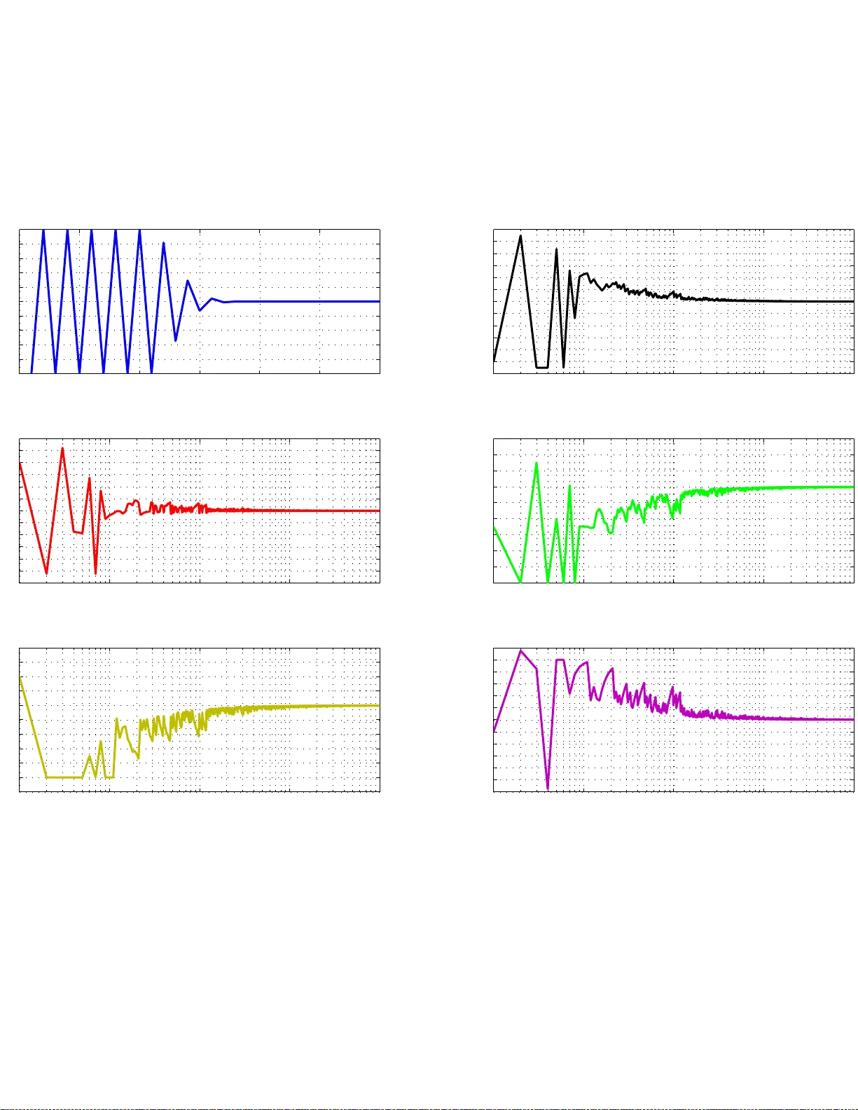
1 On distrib uted con v e x optimization under inequality and equality constraints via primal-dual subgradient methods Minghui Zhu and Sonia Mart ´ ınez Abstract W e consider a gener al multi-agen t conve x optimization problem wh ere th e agents are to collectively minimize a global objecti ve function subject to a global inequality constraint, a global equality constraint, and a glo bal co nstraint set. Th e objective function is deﬁn ed by a su m o f loc al ob jectiv e function s, while the global constraint set is produced by the intersection of local constraint sets. In p articular, we study two cases: on e where the equality co nstraint is absent, and th e other where the local con straint sets are identical. W e devise two distributed p rimal-dua l subgra dient algo rithms which are b ased on the characterizatio n of the primal-d ual o ptimal solu tions as the saddle points of the Lagrangia n and penalty function s. These alg orithms can be imp lemented over network s with changing topolo gies but satisfying a stand ard connectivity pr operty , and allow the agents to asymptotically ag ree on optim al so lutions and optimal values o f the optim ization problem u nder the Slater’ s con dition. I . I N T RO D U C T I O N Recent adva n ces i n sensing, communicati on and com putation t echnologies are challenging the way in which con trol mechanisms are designed for their ef ﬁcient exploitation in a coordinated manner . This has motiv ated a wealth of algo rithms for information processing, cooperati ve control, and opti mization of lar ge-scale networked multi-agent systems performing a v ariety of tasks. Due to a lack of a centralized authority , the proposed algorithms aim to be executed by i ndividual agents through local actio ns, with the main feature o f being rob ust to dynamic changes of network topologi es. The authors are with Depa rtment of M echanical and Aerospac e Engineering, Univ ersi ty of California, San Die go, 95 00 Gilman Dr , L a Jolla CA, 92093, { mizhu ,soniamd } @ ucsd.edu DRAFT 2 In this paper , we consi der a general multi-agent optimization p roblem where the goal is to minimize a glo bal objecti ve function, given as a su m o f local objecti ve funct ions, subject to global constrain ts, which i nclude an inequality constraint, an equality constraint and a (state) constraint set. Each local obj ectiv e function is con vex and on ly known to one particular agent. On the o ther hand, t he in equality (resp. equality) constraint is given by a con vex (resp. afﬁ n e) function and known by all agents. Each node has i ts own con ve x const raint set, and the global constraint set is deﬁned as t heir intersectio n. This problem is motiv ated by others in distributed estimation [24 ] [30], distributed s ource l ocalization [28], network util ity maxim ization [15], optimal ﬂow control in po wer systems [26], [33] and opt imal shape changes of m obile robots [9]. An imp ortant feature of t he problem i s that the o bjectiv e and (or) const raint functions depend upon a global decision vector . This requires the design of distributed algorithm s where, on the one hand, agents can align their decisions through a local information exchange and, on the other hand, the comm on decisions will coincide with an optimal s olution and the optim al value. Literatur e Review . In [2] and [32], the authors develop a general frame work for parallel and distributed computat ion over a set of processors. Consensus problem s, a class of canoni cal problems on networked multi-agent systems, hav e been intensively studied since then. A neces- sarily incom plete list of references in cludes [11], [25] tackli ng continu ous-time consensus, [5], [12], [18] in vestigati ng discrete-time versions, and [17] where asynchronous im plementation o f consensus algorithms is di scussed. The papers [6], [14], [31] treat randomized consensus via gossip commun ication, achieving consensus through qu antized informatio n and consensu s over random graphs, respectively . T he con vergence rate of consensus algorithm s is discussed, e.g., in [27], [34], and t he author in [7] derives conditions to achiev e different consensus values. In robotics and control communiti es, con vex optimization has b een exploited to desig n algo- rithms coordinatin g mobi le multi-agent systems. In [8], i n order to increase the connectivity of a multi -agent sy stem, a distributed s uper gradient-based algorithm is proposed to maximize t he second smallest eigen value of the Laplacian m atrix of the state dependent proximity graph of agents. In [9], opt imal s hape changes of mobile rob ots are achieved through second-order cone programming techni ques. In [10], a target tracking problem i s addressed by means of a generic semideﬁnite program where the constraint s of network connectivity and full target coverage are articulated as linear-matrix inequalities. In [19], in order to attain t he high est poss ible pos itioning accurac y for mobil e robots, the authors express th e cov ariance matrix of the pose errors as a DRAFT 3 functional relation of measurement frequencies, and then formu late a optimal s ensing problem as a con vex programm ing o f measurement frequencies. The recent papers [21], [23] are the most rele vant to our work. In [21], the auth ors solve a multi-agent u nconstrained con vex opt imization problem through a novel combination of a verage consensus algorith ms with subgradient methods. More recently , the paper [23] further takes local constraint sets int o account. T o deal wit h these constraints, the authors in [23] present an extension of their distributed subgradient algo rithm, by projecting the origin al algorit hm on to the local constraint sets. T wo cases are solved in [23]: the ﬁrst assumes that the network topologi es can dynamically change and satisfy a periodic s trong connectivity assum ption (i.e., the union of the network to pologies ove r a b ounded period of t ime is strongly connected), b ut then the local constraint s ets are ident ical; the second requires that the communication graphs are (ﬁxed and) comp lete and then the local constraint sets can be differ ent. Another related paper is [13] where a special case of [23], the network topo logy is ﬁxed and all the local const raint sets are identical, is addressed. Statement of Contributions. Building on the work [23], this paper furt her i ncorporates global inequality and equali ty constraints. More precisely , we stud y two cases: one in wh ich the equali ty constraint is absent, and the ot her in which the local constraint s ets are ident ical. For the ﬁrst case, we adopt a Lagrangian relaxati on approach, deﬁne a Lagrangi an dual problem and devise the distributed Lagrangian pri mal-dual subgradient algorithm (DLPDS, for short) based on the characterization of the prim al-dual o ptimal soluti ons as the saddle points of the Lagrangian function. The DLPDS algorithm in volves each agent updating its estimates of the saddle p oints via a combination of an avera g e consensus step, a sub gradient (or s upgradient) step and a primal (or dual) projectio n step onto its local constraint set (or a compact set containing the dual optimal set). The DL PDS algorithm is shown to asymptot ically conv erge to a pair o f p rimal-dual optimal s olutions und er t he Slater’ s condition and t he periodi c strong connectivity assumptio n. Furthermore, each agent asympto tically agrees on the optimal value by implement ing a dynam ic a verage cons ensus algorithm dev elop ed in [35], which allows a multi-agent system to t rack time-varying av erage values. For the second case, to di spense with the additional equality constraint, we adopt a penalty relaxation approach, while deﬁning a penalty dual pro blem and devising the distributed penalty primal-dual sub gradient algorithm (DPPDS, for short). Unlike the ﬁrst case, the dual optimal DRAFT 4 set of t he s econd case may not be bounded, and t hus th e du al projection steps are not in volved in the DPPDS algorithm. It renders t hat dual est imates and thus (prim al) subgradients may not be uniformly bounded. This challenge is add ressed by a more careful choi ce of step-sizes. W e show th at the DPPDS algorit hm asymptoti cally con ver ges to a primal op timal soluti on and the optimal value under the Slater’ s condit ion and the periodic strong connectivity assumpt ion. For the special case where the global inequality and equality constraints are not taken in to account, th is paper extends the results in [23] to a more general s cenario where the network topologies satisfy the periodi c s trong connectivity assumpt ion, and the local constraint sets can be dif ferent, wh ile relaxing an interior-point conditi on requirement. W e refer the readers to Section VI-D for addit ional in formation. I I . P RO B L E M F O R M U L A T I O N A N D A S S U M P T I O N S A. Pr oblem formulat ion Consider a network of agents labeled by V := { 1 , . . . , N } that can only interact wi th each other through local comm unication. The objective of the mul ti-agent group is to coo perativ ely solve th e fol lowing optimi zation probl em: min x ∈ R n f ( x ) := N X i =1 f [ i ] ( x ) , s . t . g ( x ) ≤ 0 , h ( x ) = 0 , x ∈ X := ∩ N i =1 X [ i ] , (1) where f [ i ] : R n → R is the con vex objective function of agent i , X [ i ] ⊆ R n is the compact and con vex constraint s et of agent i , and x i s a global decision vector . Assume t hat f [ i ] and X [ i ] are only known b y agent i , and probably different. The fun ction g : R n → R m is known to all the agents wi th each component g ℓ , for ℓ ∈ { 1 , . . . , m } , being con ve x . The inequali ty g ( x ) ≤ 0 i s understood component-wise; i.e., g ℓ ( x ) ≤ 0 , for all ℓ ∈ { 1 , . . . , m } , and represents a global inequality constraint. The function h : R n → R ν , deﬁned as h ( x ) := Ax − b with A ∈ R ν × n , represents a global equality constraint, and is known t o all t he agents. W e denote Y := { x ∈ R n | g ( x ) ≤ 0 , h ( x ) = 0 } , and assume that the set of feasible points is non-empty; i.e., X ∩ Y 6 = ∅ . Since X is compact and Y is closed, then we can deduce that X ∩ Y is com pact. The con vexity of f [ i ] implies t hat of f and thu s f is conti nuous. In this way , the op timal value p ∗ of the prob lem (1) is ﬁnite and X ∗ , the s et of primal optimal points, is non-empty . Throu ghout this paper , we sup pose the following Slater’ s condition holds: DRAFT 5 Assumption 2.1 (Slater’ s Condition): There exists a vector ¯ x ∈ X such that g ( ¯ x ) < 0 and h ( ¯ x ) = 0 . And th ere exists a relativ e interior point ˜ x of X , i.e., ˜ x ∈ X and t here exists an open sphere S centered at ˜ x such that S ∩ aﬀ ( X ) ⊂ X wit h aﬀ ( X ) bein g the afﬁne hull of X , su ch that h ( ˜ x ) = 0 . Remark 2.1: In this paper , the quantities (e.g., functions, scalars and sets) associated with agent i will be i ndexed by t he superscript [ i ] . In this paper , we will study two particular cases of prob lem (1): one in which the global equality con straint h ( x ) = 0 is not inclu ded, and the other in which all the local constrain t sets are identical. For th e case where the constraint h ( x ) = 0 is absent, the Slater’ s condition 2.1 reduces to the existence of a vector ¯ x ∈ X su ch that g ( ¯ x ) < 0 . B. Network model W e w ill cons ider that t he m ulti-agent network operates synchronously . The topology of the network at time k ≥ 0 will be represented by a directed weighted graph G ( k ) = ( V , E ( k ) , A ( k )) where A ( k ) := [ a i j ( k )] ∈ R N × N is the a d jacency matrix with a i j ( k ) ≥ 0 being the weight a ssigned to the e d ge ( j, i ) and E ( k ) ⊂ V × V \ diag( V ) is the set of edges with non-zero weights a i j ( k ) . The in-neighbors of no de i at time k are denoted by N [ i ] ( k ) = { j ∈ V | ( j, i ) ∈ E ( k ) and j 6 = i } . W e here make the follo wing ass umptions on the network communication graphs, which are standard in the analys is of avera g e consensus algo rithms; e.g., see [25], [27], and distributed optim ization in [21], [23]. Assumption 2.2 (Non-degeneracy): There exists a const ant α > 0 su ch that a i i ( k ) ≥ α , and a i j ( k ) , for i 6 = j , satisﬁes a i j ( k ) ∈ { 0 } ∪ [ α, 1] , for all k ≥ 0 . Assumption 2.3 (Balanced Communication): 1 It hol ds that P N j =1 a i j ( k ) = 1 for all i ∈ V and k ≥ 0 , and P N i =1 a i j ( k ) = 1 for all j ∈ V and k ≥ 0 . Assumption 2.4 (Pe riodical Str ong Connectivity): There is a positive integer B such t hat, for all k 0 ≥ 0 , the directed graph ( V , S B − 1 k =0 E ( k 0 + k )) is strongl y connected. C. Notion and nota tions The following notion of saddl e p oint plays a critical rol e i n our paper . 1 It is also referred to as double stochasticity . DRAFT 6 Deﬁnition 2.1 (Saddle point): Consider a function φ : X × M → R where X and M are non-empty subsets of R ¯ n and R ¯ m . A pair of vectors ( x ∗ , µ ∗ ) ∈ X × M is called a sadd le point of φ over X × M if φ ( x ∗ , µ ) ≤ φ ( x ∗ , µ ∗ ) ≤ φ ( x, µ ∗ ) hold for all ( x, µ ) ∈ X × M . Remark 2.2: Equiv alently , ( x ∗ , µ ∗ ) i s a saddle po int of φ over X × M if and only i f ( x ∗ , µ ∗ ) ∈ X × M , and sup µ ∈ M φ ( x ∗ , µ ) ≤ φ ( x ∗ , µ ∗ ) ≤ inf x ∈ X φ ( x, µ ∗ ) . • In t his paper , we do not assume the dif ferentiabi lity of f [ i ] and g ℓ . A t the points where the function i s not differentiable, the sub gradient plays the role of the gradient. For a given con ve x function F : R ¯ n → R and a point ˜ x ∈ R ¯ n , a su bgradient of the fun ction F at ˜ x is a vector D F ( ˜ x ) ∈ R ¯ n such that the fol lowing subgradient inequality holds for any x ∈ R ¯ n : D F ( ˜ x ) T ( x − ˜ x ) ≤ F ( x ) − F ( ˜ x ) . Similarly , for a giv en concave function G : R ¯ m → R and a point ¯ µ ∈ R ¯ m , a supgradient of the function G at ¯ µ is a vector D G ( ¯ µ ) ∈ R ¯ m such t hat the following su pgradient inequality holds for any µ ∈ R ¯ m : D G ( ¯ µ ) T ( µ − ¯ µ ) ≥ G ( µ ) − G ( ¯ µ ) . Giv en a set S , we d enote by co( S ) its con vex hull. W e let the function [ · ] + : R ¯ m → R ¯ m ≥ 0 denote the projection operator on to the non-negative orthant in R ¯ m . For any vector c ∈ R ¯ n , we denote | c | := ( | c 1 | , · · · , | c ¯ n | ) T , while k · k is the 2-norm in the Euclidean s pace. I I I . C A S E ( I ) : A B S E N C E O F E Q UA L I T Y C O N S T R A I N T In this section, we study the case of problem (1) where t he equality constraint h ( x ) = 0 is absent; i.e., problem (1) b ecomes min x ∈ R n N X i =1 f [ i ] ( x ) , s . t . g ( x ) ≤ 0 , x ∈ ∩ N i =1 X [ i ] . (2) W e ﬁrst provide some prelimi naries, in cluding a Lagrangian saddle-point characterization of problem (2) and ﬁnding a su perset contai ning the Lagrangian du al opt imal set of prob lem (2 ). After that, we present t he dis tributed Lagrangian primal-dual subg radient algorithm and summa- rize its con ver gence properties. A. Pr elimin aries W e here de velop some prelim inary results which are essenti al to the design of the distri buted Lagrangian primal-dual subgradient algorith m. DRAFT 7 1) A Lagrangian saddle-poin t characterization: Firstly , problem (2) i s equiv alent to min x ∈ R n f ( x ) , s . t . N g ( x ) ≤ 0 , x ∈ X , with associated Lagrangian dual problem given by max µ ∈ R m q L ( µ ) , s . t . µ ≥ 0 . Here, the Lagrangian dual functio n, q L : R m ≥ 0 → R , is deﬁned as q L ( µ ) := inf x ∈ X L ( x, µ ) , where L : R n × R m ≥ 0 → R is the La grangia n function L ( x, µ ) = f ( x ) + N µ T g ( x ) . W e denote the Lagrangian dual optimal value of the Lagrangian dual probl em by d ∗ L and the set of Lagrangian dual optim al points by D ∗ L . As is well-known, under the Slater’ s condition 2.1, the property of strong duality holds ; i.e., p ∗ = d ∗ L , and D ∗ L 6 = ∅ . The following theorem is a standard result on L agrangian duality stating that the prim al and Lagrangian dual optim al solut ions can be characterized as the saddle po ints of the Lagrangian function. Theor em 3.1 (Lagrangian Saddle-point The o r em [3]): The pair of ( x ∗ , µ ∗ ) ∈ X × R m ≥ 0 is a saddle point of t he Lagrangian function L ove r X × R m ≥ 0 if and only if i t i s a p air of p rimal and Lagrangian dual opt imal s olutions and the following Lagrangian m inimax equality holds: sup µ ∈ R m ≥ 0 inf x ∈ X L ( x, µ ) = inf x ∈ X sup µ ∈ R m ≥ 0 L ( x, µ ) . This following lemma presents som e p reliminary analysis of Lagrangian saddl e po ints. Lemma 3 .1 (Pre l iminary results of Lagrangian saddle points): Let M be any superset of D ∗ L . (a) If ( x ∗ , µ ∗ ) is a saddl e point of L over X × R m ≥ 0 , then ( x ∗ , µ ∗ ) is also a saddle point of L over X × M . (b) There is at least one s addle point of L over X × M . (c) If ( ˇ x, ˇ µ ) is a saddle point of L over X × M , then L ( ˇ x, ˇ µ ) = p ∗ and ˇ µ is Lagrangian dual optimal. Pr oof: (a) It just fol lows from the deﬁnition of saddl e p oint of L over X × M . (b) Observe that sup µ ∈ R m ≥ 0 inf x ∈ X L ( x, µ ) = sup µ ∈ R m ≥ 0 q L ( µ ) = d ∗ L , inf x ∈ X sup µ ∈ R m ≥ 0 L ( x, µ ) = inf x ∈ X ∩ Y f ( x ) = p ∗ . DRAFT 8 Since t he Slater’ s condition 2.1 implies zero duality gap, t he L agrangian mi nimax equ ality ho lds. From Theorem 3.1 it foll ows that the set of saddle points of L over X × R m ≥ 0 is the Cartesian product X ∗ × D ∗ L . Recall that X ∗ and D ∗ L are non-emp ty , so w e can guarantee the existence o f the saddle point of L over X × R m ≥ 0 . Then by (a), we have th at (b) holds. (c) Pick any saddl e point ( x ∗ , µ ∗ ) of L over X × R m ≥ 0 . Since t he Slater’ s condition 2.1 holds, from Theorem 3.1 one can deduce that ( x ∗ , µ ∗ ) is a pair of primal and Lagrangian dual o ptimal solutions . This im plies t hat d ∗ L = inf x ∈ X L ( x, µ ∗ ) ≤ L ( x ∗ , µ ∗ ) ≤ sup µ ∈ R m ≥ 0 L ( x ∗ , µ ) = p ∗ . From Theorem 3.1 , we ha ve d ∗ L = p ∗ . Hence, L ( x ∗ , µ ∗ ) = p ∗ . On the other h and, we pick any saddle po int ( ˇ x, ˇ µ ) of L ove r X × M . Then for all x ∈ X and µ ∈ M , it hold s that L ( ˇ x, µ ) ≤ L ( ˇ x, ˇ µ ) ≤ L ( x, ˇ µ ) . By Theorem 3.1 , then µ ∗ ∈ D ∗ L ⊆ M . Recall x ∗ ∈ X , and thus we hav e L ( ˇ x, µ ∗ ) ≤ L ( ˇ x, ˇ µ ) ≤ L ( x ∗ , ˇ µ ) . Since ˇ x ∈ X and ˇ µ ∈ R m ≥ 0 , we have L ( x ∗ , ˇ µ ) ≤ L ( x ∗ , µ ∗ ) ≤ L ( ˇ x, µ ∗ ) . Comb ining the above two relations g iv es that L ( ˇ x, ˇ µ ) = L ( x ∗ , µ ∗ ) = p ∗ . From Remark 2.2 we see that L ( ˇ x, ˇ µ ) ≤ inf x ∈ X L ( x, ˇ µ ) = q L ( ˇ µ ) . Since L ( ˇ x, ˇ µ ) = p ∗ = d ∗ L ≥ q L ( ˇ µ ) , then q L ( ˇ µ ) = d ∗ L and thus ˇ µ is a Lagrangian dual optimal solution. Remark 3.1: Despite that (c) holds, the rev erse of (a) may not be true in general. In particular , x ∗ may be infeasible; i.e., g ℓ ( x ∗ ) > 0 for some ℓ ∈ { 1 , . . . , m } . • 2) A upper estimate of the Lagrangian dual optimal set: In what follows, we will ﬁnd a compact superset of D ∗ L . T o do that, we deﬁne the following primal problem for each agent i : min x ∈ R n f [ i ] ( x ) , s . t . g ( x ) ≤ 0 , x ∈ X [ i ] . Due to the fact that X [ i ] is compact and th e f [ i ] are continuo us, th e primal optim al value p ∗ i of each agent’ s p rimal problem is ﬁnite and the set of its p rimal opt imal solut ions is non-emp ty . The associated dual probl em is giv en by max µ ∈ R m q [ i ] ( µ ) , s . t . µ ≥ 0 . Here, the du al function q [ i ] : R m ≥ 0 → R is d eﬁned by q [ i ] ( µ ) := inf x ∈ X [ i ] L [ i ] ( x, µ ) , where L [ i ] : R n × R m ≥ 0 → R is th e Lagrangian function o f agent i and giv en by L [ i ] ( x, µ ) = f [ i ] ( x ) + µ T g ( x ) . The corresponding dual optimal va l ue i s denoted by d ∗ i . In this way , L is decomposed i nto a sum of local Lagrangian functi ons; i.e., L ( x, µ ) = P N i =1 L [ i ] ( x, µ ) . DRAFT 9 Deﬁne now the s et-va lued map Q : R m ≥ 0 → 2 ( R m ≥ 0 ) by Q ( ˜ µ ) = { µ ∈ R m ≥ 0 | q L ( µ ) ≥ q L ( ˜ µ ) } . Additionall y , deﬁne a function γ : X → R b y γ ( x ) = min ℓ ∈{ 1 ,...,m } {− g ℓ ( x ) } . Obs erve th at if x is a Slater vector , then γ ( x ) > 0 . The following lemma is a d irect resul t of Lemma 1 in [20]. Lemma 3 .2 (Boundedn ess of dual solution sets): The set Q ( ˜ µ ) is bounded for any ˜ µ ∈ R m ≥ 0 , and, in particular , for any Slater vector ¯ x , it hol ds that max µ ∈ Q ( ˜ µ ) k µ k ≤ 1 γ ( ¯ x ) ( f ( ¯ x ) − q L ( ˜ µ )) .  Notice that D ∗ L = { µ ∈ R m ≥ 0 | q L ( µ ) ≥ d ∗ L } . Picking any Slater vector ¯ x ∈ X , and lettin g ˜ µ = µ ∗ ∈ D ∗ L in Lemma 3.2 gives that max µ ∗ ∈ D ∗ L k µ ∗ k ≤ 1 γ ( ¯ x ) ( f ( ¯ x ) − d ∗ L ) . (3) Deﬁne the functi on r : X × R m ≥ 0 → R ∪ { + ∞ } by r ( x, µ ) := N γ ( x ) max i ∈ V { f [ i ] ( x ) − q [ i ] ( µ ) } . By the property of weak duality , it holds that d ∗ i ≤ p ∗ i and thus f [ i ] ( x ) ≥ q [ i ] ( µ ) for any ( x, µ ) ∈ X × R m ≥ 0 . Since γ ( ¯ x ) > 0 , thus r ( ¯ x, µ ) ≥ 0 for any µ ∈ R m ≥ 0 . W i th this observ atio n, we pick any ˜ µ ∈ R m ≥ 0 and the following s et is well-deﬁned: ¯ M [ i ] ( ¯ x , ˜ µ ) := { µ ∈ R m ≥ 0 | k µ k ≤ r ( ¯ x, ˜ µ ) + θ [ i ] } for some θ [ i ] ∈ R > 0 . Observe th at for all µ ∈ R m ≥ 0 : q L ( µ ) = inf x ∈∩ N i =1 X [ i ] N X i =1 ( f [ i ] ( x ) + µ T g ( x )) ≥ N X i =1 inf x ∈ X [ i ] ( f [ i ] ( x ) + µ T g ( x )) = N X i =1 q [ i ] ( µ ) . (4) Since d ∗ L ≥ q L ( ˜ µ ) , it follows from (3) and (4) th at max µ ∗ ∈ D ∗ L k µ ∗ k ≤ 1 γ ( ¯ x ) ( f ( ¯ x ) − q L ( ˜ µ )) ≤ 1 γ ( ¯ x ) ( f ( ¯ x ) − N X i =1 q [ i ] ( ˜ µ )) ≤ N γ ( ¯ x ) max i ∈ V { f [ i ] ( ¯ x ) − q [ i ] ( ˜ µ ) } = r ( ¯ x, ˜ µ ) . Hence, we hav e D ∗ L ⊆ ¯ M [ i ] ( ¯ x, ˜ µ ) for all i ∈ V . Note th at in order to compute ¯ M [ i ] ( ¯ x, ˜ µ ) , all the agents ha ve t o agre e on a common Slater vector ¯ x ∈ ∩ N i =1 X [ i ] which should be o btained in a distrib u ted fashion. T o handle this difﬁculty , we now propo se a di stributed algorit hm, namely Dis tributed Sl ater-ve ct or Computati on Algorithm , which allows each agent i t o compute a sup erset o f ¯ M [ i ] ( ¯ x, ˜ µ ) . Initially , each agent i chooses a commo n value ˜ µ ∈ R m ≥ 0 ; e.g., ˜ µ = 0 , and computes tw o positive const ants b [ i ] (0) and c [ i ] (0) such that b [ i ] (0) ≥ sup x ∈ J [ i ] { f [ i ] ( x ) − q [ i ] ( ˜ µ ) } and c [ i ] (0) ≤ min 1 ≤ ℓ ≤ m inf x ∈ J [ i ] {− g ℓ ( x ) } where J [ i ] := { x ∈ X [ i ] | g ( x ) < 0 } . DRAFT 10 At e very time k ≥ 0 , each agent i up dates its estimates by using the following rules: b [ i ] ( k + 1) = max j ∈N [ i ] ( k ) ∪{ i } b [ j ] ( k ) , c [ i ] ( k + 1) = min j ∈N [ i ] ( k ) ∪{ i } c [ j ] ( k ) . Lemma 3 .3 (Con vergen ce pr operties of the dis trib uted Slater -vector Comput ation Algorithm): Assume that the periodical strong connectivity assumpt ion 2.4 h olds. Consider the sequences of { b [ i ] ( k ) } and { c [ i ] ( k ) } generated by th e Distributed Slater -vector Computation Algorit hm. It holds that after at m ost ( N − 1 ) B steps, all the agents reach the consensus, i .e., b [ i ] ( k ) = b ∗ := max j ∈ V b [ j ] (0) and c [ i ] ( k ) = c ∗ := min j ∈ V c [ j ] (0) for all k ≥ ( N − 1) B . Furthermore, we ha ve M [ i ] ( ˜ µ ) := { µ ∈ R m ≥ 0 | k µ k ≤ N b ∗ c ∗ + θ [ i ] } ⊇ ¯ M [ i ] ( ¯ x , ˜ µ ) for i ∈ V . Pr oof: It is not dif ﬁcult to v erify achieving max-consensus and m in-consensus b y using the periodical strong connectivity assumption 2.4. Note that J := { x ∈ X | g ( x ) < 0 } ⊆ J [ i ] , ∀ i ∈ V . Hence, we have max i ∈ V sup x ∈ J { f [ i ] ( x ) − q [ i ] ( ˜ µ ) } ≤ max i ∈ V sup x ∈ J [ i ] { f [ i ] ( x ) − q [ i ] ( ˜ µ ) } ≤ b ∗ , inf x ∈ J min 1 ≤ ℓ ≤ m {− g ℓ ( x ) } ≥ min i ∈ V inf x ∈ J [ i ] min 1 ≤ ℓ ≤ m {− g ℓ ( x ) } ≥ c ∗ . Since ¯ x ∈ J , then th e fol lowing estimate on r ( ¯ x, ˜ µ ) hold s: r ( ¯ x, ˜ µ ) ≤ N sup x ∈ J max i ∈ V { f [ i ] ( x ) − q [ i ] ( ˜ µ ) } inf x ∈ J min 1 ≤ ℓ ≤ m {− g ℓ ( x ) } ≤ N b ∗ c ∗ . The desired result im mediately follows. From Lemm a 3.3 and the f act that D ∗ L ⊆ ¯ M [ i ] ( ¯ x , ˜ µ ) , we can see that the set of M ( ˜ µ ) := ∩ N i =1 M [ i ] ( ˜ µ ) contains D ∗ L . In addit ion, M [ i ] ( ˜ µ ) and M ( ˜ µ ) are non-emp ty , compact and con vex. T o simplify the notations, we will use the shorthands M [ i ] := M [ i ] ( ˜ µ ) and M := M ( ˜ µ ) . 3) Con ve xity of L : For each µ ∈ R m ≥ 0 , w e deﬁne the function L [ i ] µ : R n → R as L [ i ] µ ( x ) := L [ i ] ( x, µ ) . Note that L [ i ] µ is con vex since it is a n onnegati ve weighted sum of con vex functions. For each x ∈ R n , we deﬁne the function L [ i ] x : R m ≥ 0 → R as L [ i ] x ( µ ) := L [ i ] ( x, µ ) . It is easy to check that L [ i ] x is a concave (actually af ﬁne) function. Then th e Lagrangian function L i s the sum o f a collection of con vex-c o nca ve l ocal function s. This property mot iv ates us to signiﬁcantly extend prim al-dual subgradient methods in [1], [22] to th e networked multi -agent scenario. B. Distri buted Lagrangian primal-dual subgradient algorithm Here, we introd uce t he Distributed Lagrangian Primal-Dual Subgradient Algo rithm (DLPDS, for short) t o ﬁnd a saddle point of the Lagrangian function L over X × M and the optim al value. DRAFT 11 This saddle point will coincide with a pair of primal and Lagrangian dual optim al solutions which is not always th e case; see Remark 3.1. Through the algorithm , at each time k , each agent i maintains the estimate of ( x [ i ] ( k ) , µ [ i ] ( k )) to th e s addle point of the Lagrangian functi on L over X × M and the estimate of y [ i ] ( k ) to p ∗ . T o produce x [ i ] ( k + 1) (resp. µ [ i ] ( k + 1) ), agent i takes a con ve x combi nation v [ i ] x ( k ) (resp. v [ i ] µ ( k ) ) of its estimate x [ i ] ( k ) (resp. µ [ i ] ( k ) ) wi th the estimates sent from its neighbo ring agents at time k , makes a su bgradient (resp. supgradient) step to minimize (resp. m aximize) the local Lagrangian function L [ i ] , and t akes a primal (resp. dual) projection ont o the local constraint X [ i ] (resp. M [ i ] ). Furthermore, agent i g enerates t he esti mate y [ i ] ( k + 1) by t aking a con vex com bination v [ i ] y ( k ) of its estimat e y [ i ] ( k ) wit h the esti mates of its neighbors at t ime k and taking one step t o track the var i ation of the local objectiv e function f [ i ] . The DLPDS algorithm is formally stated as follows: Initially , each agent i picks a common ˜ µ ∈ R m ≥ 0 and computes t he set M [ i ] with some θ [ i ] > 0 by using the Distributed Slater-vector Compu tation Algorithm. Furthermore, agent i chooses any initial state x [ i ] (0) ∈ X [ i ] , µ [ i ] (0) ∈ R m ≥ 0 , and y [ i ] (1) = N f [ i ] ( x [ i ] (0)) . At ev ery k ≥ 0 , each agent i generates x [ i ] ( k + 1) , µ [ i ] ( k + 1) and y [ i ] ( k + 1) according to the following rules: v [ i ] x ( k ) = N X j =1 a i j ( k ) x [ j ] ( k ) , v [ i ] µ ( k ) = N X j =1 a i j ( k ) µ [ j ] ( k ) , v [ i ] y ( k ) = N X j =1 a i j ( k ) y [ j ] ( k ) , x [ i ] ( k + 1) = P X [ i ] [ v [ i ] x ( k ) − α ( k ) D [ i ] x ( k )] , µ [ i ] ( k + 1) = P M [ i ] [ v [ i ] µ ( k ) + α ( k ) D [ i ] µ ( k )] , y [ i ] ( k + 1) = v [ i ] y ( k ) + N ( f [ i ] ( x [ i ] ( k )) − f [ i ] ( x [ i ] ( k − 1))) , where P X [ i ] (resp. P M [ i ] ) is the projection operator onto the set X [ i ] (resp. M [ i ] ), the scalars a i j ( k ) are non-negati ve weights and the scalars α ( k ) > 0 are step-sizes 2 . W e use the s horthands D [ i ] x ( k ) ≡ D L [ i ] v [ i ] µ ( k ) ( v [ i ] x ( k )) , and D [ i ] µ ( k ) ≡ D L [ i ] v [ i ] x ( k ) ( v [ i ] µ ( k )) . The following theorem sum marizes the conv ergence properties of the DLPDS al gorithm where agents asymptoticall y agree u pon a pair of primal-dual opti mal so lutions. Theor em 3.2 (Con vergence pr operties of the DLPDS algorithm): Consider the optimiza- tion problem (2). Let the non-degeneracy assumpt ion 2.2, the balanced communication assump- tion 2 .3 and the periodic strong connectivity assu mptions 2.4 hold. Consider t he s equences of 2 Each agent i executes the update law of y [ i ] ( k ) for k ≥ 1 . DRAFT 12 { x [ i ] ( k ) } , { µ [ i ] ( k ) } and { y [ i ] ( k ) } of the di stributed Lagrangian p rimal-dual subgradi ent algorit hm with the s tep-sizes { α ( k ) } s atisfying lim k → + ∞ α ( k ) = 0 , + ∞ X k =0 α ( k ) = + ∞ , and + ∞ X k =0 α ( k ) 2 < + ∞ . Then, there is a pair o f pri mal and Lagrangian dual optimal solutions ( x ∗ , µ ∗ ) ∈ X ∗ × D ∗ L such that lim k → + ∞ k x [ i ] ( k ) − x ∗ k = 0 and lim k → + ∞ k µ [ i ] ( k ) − µ ∗ k = 0 for all i ∈ V . Furtherm ore, we hav e that lim k → + ∞ k y [ i ] ( k ) − p ∗ k = 0 for all i ∈ V . Remark 3.2: For a con vex-c o nca ve function , contin uous-time g radient-based meth ods are proved in [1] to con verge globally tow ards the saddle-point. Recently , [22] presents (di screte- time) primal-dual subgradient methods which relax th e diff erentiability in [1] and further incor- porate state constraints. The method in [1] i s adopted by [16 ] and [29] to study a distributed optimizatio n problem on ﬁxed graphs where objective functions are separable. The DLPDS algorith m is a generalization of prim al-dual subgradient methods in [22] to the networked multi-agent scenario. It is also an extension of the di stributed projected su bgradient algorithm i n [23] to solve multi-agent con vex optim ization problems with inequalit y constraints. Additionall y , the DLPDS algorithm enables agents t o ﬁnd t he optim al value. Furthermore, the DLPDS algorithm objective is that of reaching a saddle point of the Lagrangian function in contrast to achieving a (primal) optimal solution in [23]. • I V . C A S E ( I I ) : I D E N T I C A L L O C A L C O N S T R A I N T S E T S In last section, we st udy the case where the equalit y constraint is absent in problem (1). In this section, we turn our attent ion to another case o f problem (1) where h ( x ) = 0 is taken int o account but we require that local constraint sets are i dentical; i.e., X [ i ] = X for all i ∈ V . W e ﬁrst adopt a penalty relaxation and provide a p enalty saddle-point characterization of primal problem (1) wi th X [ i ] = X . W e then introduce t he distributed penalty primal-dual s ubgradient algorithm, followed by its con vergence properties and some remarks. A. Pr elimin aries Some prelimi nary resul ts are presented in thi s part, and t hese results are essential t o the dev elopm ent of the di stributed penalty primal-dual subg radient algorithm. DRAFT 13 1) A penalty saddle-point characterization: Note that the primal probl em (1) with X [ i ] = X is trivially equiv alent to the following: min x ∈ R n f ( x ) , s . t . N g ( x ) ≤ 0 , N h ( x ) = 0 , x ∈ X , (5) with associated penalty dual probl em giv en by max µ ∈ R m ,λ ∈ R ν q P ( µ, λ ) , s . t . µ ≥ 0 , λ ≥ 0 . (6) Here, t he penalty dual function, q P : R m ≥ 0 × R ν ≥ 0 → R , is deﬁned by q P ( µ, λ ) := inf x ∈ X H ( x, µ, λ ) , where H : R n × R m ≥ 0 × R ν ≥ 0 → R is the penalty fu nction g iv en by H ( x, µ, λ ) = f ( x ) + N µ T [ g ( x )] + + N λ T | h ( x ) | . W e denote t he penalty dual o ptimal value by d ∗ P and the set of penalty dual optimal solu tions by D ∗ P . W e deﬁne the penalty functio n H [ i ] ( x, µ, λ ) : R n × R m ≥ 0 × R ν ≥ 0 → R for each agent i as follows: H [ i ] ( x, µ, λ ) = f [ i ] ( x ) + µ T [ g ( x )] + + λ T | h ( x ) | . In this way , we hav e that H ( x, µ, λ ) = P N i =1 H [ i ] ( x, µ, λ ) . As prov en in the next lemma, the Slater’ s condition 2.1 ensures zero duality gap and t he existence of penalty du al optimal soluti ons. Lemma 4 .1 (Str ong duality and non-emptyness of the penalty dual optimal set): The v al - ues of p ∗ and d ∗ P coincide, and D ∗ P is non-empt y . Pr oof: Consider the auxiliary Lagrangi an function L a : R n × R m ≥ 0 × R ν → R gi ven b y L a ( x, µ, λ ) = f ( x ) + N µ T g ( x ) + N λ T h ( x ) , with the associated dual probl em deﬁned by max µ ∈ R m ,λ ∈ R ν q a ( µ, λ ) , s . t . µ ≥ 0 . (7) Here, t he dual function, q a : R m ≥ 0 × R ν → R , is deﬁned by q a ( µ, λ ) := inf x ∈ X L a ( x, µ, λ ) . The dual optimal v alue of problem (7) i s denoted by d ∗ a and the set of dual optim al s olutions is denoted D ∗ a . Since X is con vex, f and g ℓ , for ℓ ∈ { 1 , . . . , m } , are con vex, p ∗ is ﬁnite and the Slater’ s con dition 2 .1 ho lds, it follows from Propositio n 5.3.5 in [3] that p ∗ = d ∗ a and D ∗ a 6 = ∅ . W e now proceed to characterize d ∗ P and D ∗ P . Pick any ( µ ∗ , λ ∗ ) ∈ D ∗ a . Since µ ∗ ≥ 0 , then d ∗ a = q a ( µ ∗ , λ ∗ ) = inf x ∈ X { f ( x ) + N ( µ ∗ ) T g ( x ) + N ( λ ∗ ) T h ( x ) } ≤ inf x ∈ X { f ( x ) + N ( µ ∗ ) T [ g ( x )] + + N | λ ∗ | T | h ( x ) |} = q P ( µ ∗ , | λ ∗ | ) ≤ d ∗ P . (8) On the other hand, pick any x ∗ ∈ X ∗ . Then x ∗ is feasible, i.e., x ∗ ∈ X , [ g ( x ∗ )] + = 0 and | h ( x ∗ ) | = 0 . It imp lies that q P ( µ, λ ) ≤ H ( x ∗ , µ, λ ) = f ( x ∗ ) = p ∗ holds fo r any µ ∈ R m ≥ 0 and λ ∈ R ν ≥ 0 , and thus d ∗ P = sup µ ∈ R m ≥ 0 ,λ ∈ R ν ≥ 0 q P ( µ, λ ) ≤ p ∗ = d ∗ a . Therefore, we have d ∗ P = p ∗ . DRAFT 14 T o prove t he emptyness of D ∗ P , we pick any ( µ ∗ , λ ∗ ) ∈ D ∗ a . From (8) and d ∗ a = d ∗ P , we can see that ( µ ∗ , | λ ∗ | ) ∈ D ∗ P and thus D ∗ P 6 = ∅ . The following is a sl ight extension of Theorem 3.1 to penalty functions. Theor em 4.1 (Penalty Saddle-point Theor em): The pair of ( x ∗ , µ ∗ , λ ∗ ) is a saddle p oint of the penalty functio n H over X × R m ≥ 0 × R ν ≥ 0 if and only if i t is a pair of p rimal and penalty dual optimal solut ions and th e following penalty mini max equ ality holds: sup ( µ,λ ) ∈ R m ≥ 0 × R ν ≥ 0 inf x ∈ X H ( x, µ, λ ) = inf x ∈ X sup ( µ,λ ) ∈ R m ≥ 0 × R ν ≥ 0 H ( x, µ, λ ) . Pr oof: The proof is analogous to that of Proposition 6.2.4 in [4], and for the sake of completeness, we pro vi de the details here. It follo ws from Proposition 2.6. 1 in [4] that ( x ∗ , µ ∗ , λ ∗ ) is a saddle point of H over X × R m ≥ 0 × R ν ≥ 0 if and only if the penalty minimax equality holds and the following conditi ons are satisﬁed: sup ( µ,λ ) ∈ R m ≥ 0 × R ν ≥ 0 H ( x ∗ , µ, λ ) = min x ∈ X { sup ( µ,λ ) ∈ R m ≥ 0 × R ν ≥ 0 H ( x, µ, λ ) } , (9) inf x ∈ X H ( x, µ ∗ , λ ∗ ) = max ( µ,λ ) ∈ R m ≥ 0 × R ν ≥ 0 { inf x ∈ X H ( x, µ, λ ) } . (10) Notice that inf x ∈ X H ( x, µ, λ ) = q P ( µ, λ ) ; a n d if x ∈ Y , then sup ( µ,λ ) ∈ R m ≥ 0 × R ν ≥ 0 H ( x, µ, λ ) = f ( x ) , otherwise, sup ( µ,λ ) ∈ R m ≥ 0 × R ν ≥ 0 H ( x, µ, λ ) = + ∞ . Hence, the penalty mi nimax equality is equiv alent to d ∗ P = p ∗ . Condition (9) is equiv alent t o the fact that x ∗ is prim al optimal, and condit ion (10) is equiv alent to ( µ ∗ , λ ∗ ) being a penalty dual opti mal solution . 2) Con ve xity of H : Since g ℓ is con ve x and [ · ] + is con ve x and n on-decreasing, th us [ g ℓ ( x )] + is con vex in x for each ℓ ∈ { 1 , . . . , m } . Deno te A := ( a T 1 , · · · , a T ν ) T . Since | · | i s con vex and a T ℓ x − b ℓ is an afﬁ n e mapping, then | a T ℓ x − b ℓ | is con vex in x for each ℓ ∈ { 1 , . . . , ν } . W e denote w := ( µ, λ ) . F o r each w ∈ R m ≥ 0 × R ν ≥ 0 , we deﬁne the function H [ i ] w : R n → R as H [ i ] w ( x ) := H [ i ] ( x, w ) . Note that H [ i ] w ( x ) is con vex in x b y using the fact t hat a nonnegati ve weighted sum of con vex functio ns is con ve x. For each x ∈ R n , we deﬁne the function H [ i ] x : R m ≥ 0 × R ν ≥ 0 → R as H [ i ] x ( w ) := H [ i ] ( x, w ) . It is easy to check t hat H [ i ] x ( w ) i s concave (actually af ﬁne) i n w . Then the p enalty function H ( x, w ) i s the sum of con vex-conca ve l ocal functions. Remark 4.1: The Lagra ngian relaxation do es not ﬁt to o ur a pproach here since the La grangian function is not con vex in x by allowing λ entries t o be negati ve. • DRAFT 15 B. Distri buted p enalty primal -dual subgradient algorit hm W e are no w in the p osition to devise the Distr ibuted P enalty Primal-Dual Subgradient Al- gorithm (DPPDS, for short), th at is based on t he penalty saddle-point theorem 4.1, to ﬁnd th e optimal value and a pri mal opt imal s olution t o primal probl em (1) wi th X [ i ] = X . The DPPDS algorithm is formally described as fol low . Initially , agent i chooses any initi al state x [ i ] (0) ∈ X , µ [ i ] (0) ∈ R m ≥ 0 , λ [ i ] (0) ∈ R ν ≥ 0 , and y [ i ] (1) = N f [ i ] ( x [ i ] (0)) . At ev ery time k ≥ 0 , each agent i comput es th e following con vex combinations : v [ i ] x ( k ) = N X j =1 a i j ( k ) x [ j ] ( k ) , v [ i ] y ( k ) = N X j =1 a i j ( k ) y [ j ] ( k ) , v [ i ] µ ( k ) = N X j =1 a i j ( k ) µ [ j ] ( k ) , v [ i ] λ ( k ) = N X j =1 a i j ( k ) λ [ j ] ( k ) , and generates x [ i ] ( k + 1) , y [ i ] ( k + 1) , µ [ i ] ( k + 1) and λ [ i ] ( k + 1 ) according t o the following rules: x [ i ] ( k + 1) = P X [ v [ i ] x ( k ) − α ( k ) S [ i ] x ( k )] , y [ i ] ( k + 1) = v [ i ] y ( k ) + N ( f [ i ] ( x [ i ] ( k )) − f [ i ] ( x [ i ] ( k − 1)) ) , µ [ i ] ( k + 1) = v [ i ] µ ( k ) + α ( k )[ g ( v [ i ] x ( k ))] + , λ [ i ] ( k + 1) = v [ i ] λ ( k ) + α ( k ) | h ( v [ i ] x ( k )) | , where P X is the projection operator o nto the set X , the scalars a i j ( k ) are no n-negati ve weights and the positive scalars { α ( k ) } are step-si zes 3 . The vector S [ i ] x ( k ) := D f [ i ] ( v [ i ] x ( k )) + m X ℓ =1 v [ i ] µ ( k ) ℓ D [ g ℓ ( v [ i ] x ( k ))] + + ν X ℓ =1 v [ i ] λ ( k ) ℓ D | h ℓ | ( v [ i ] x ( k )) is a subgradient of H [ i ] w [ i ] ( k ) ( x ) at x = v [ i ] x ( k ) where w [ i ] ( k ) := ( v [ i ] µ ( k ) , v [ i ] λ ( k )) is the con vex combination of dual estimat es o f agent i and its neighb ors’. Giv en a s tep-size sequence { α ( k ) } , we deﬁne its sum over [0 , k ] by s ( k ) := P k ℓ =0 α ( ℓ ) and assume that: Assumption 4.1 (Step-size assumption): The step-sizes satisfy lim k → + ∞ α ( k ) = 0 , P + ∞ k =0 α ( k ) = + ∞ , P + ∞ k =0 α ( k ) 2 < + ∞ , and lim k → + ∞ α ( k + 1) s ( k ) = 0 , P + ∞ k =0 α ( k + 1) 2 s ( k ) < + ∞ , P + ∞ k =0 α ( k + 1) 2 s ( k ) 2 < + ∞ . 3 Each agent i executes the update law of y [ i ] ( k ) for k ≥ 1 . DRAFT 16 The following t heorem is the main result of this s ection, characterizing con vergence properties of the DPPDS algorithm where a optimal solution and the optimal v alue are a symptoti cally agreed upon. Theor em 4.2 (Con vergence pr operties of the DPPDS algorithm): Consider the problem (1) with X [ i ] = X . Let the n on-degenerac y assumption 2.2, the balanced communication assump- tion 2.3 and the periodic strong connecti vity assum ption 2.4 ho ld. Consi der the sequences of { x [ i ] ( k ) } and { y [ i ] ( k ) } of t he distributed penalt y primal-dual subgradient algorithm where the step-sizes { α ( k ) } satisfy the step-size assumpti on 4.1. Then there exists a primal opti- mal s olution ˜ x ∈ X ∗ such that lim k → + ∞ k x [ i ] ( k ) − ˜ x k = 0 for all i ∈ V . Furthermore, we hav e lim k → + ∞ k y [ i ] ( k ) − p ∗ k = 0 for all i ∈ V . W e here provide som e remarks to conclude this sectio n,. Remark 4.2: As primal-dual (sub)gradient algorithm in [1], [22], the DPPDS algorithm pro- duces a pair of primal and dual esti mates at each s tep. Main dif ferences include: ﬁrstly , the DPPDS algorit hm extends the primal-dual subgradient algorithm i n [22] t o the multi-agent scenario; s econdly , it further takes the equality con straint into account. The presence of the equality c onstraint can make D ∗ P unbounded. Therefore , unlike the DLPDS algorithm, the DPPDS algorithm does not in volve t he dual proj ection steps ont o compact sets. This may cause the subgradient S [ i ] x ( k ) not to be uniformly bounded, while the boundedness of subgradients is a standard assumpti on i n the analysis of subgradient meth ods, e.g., see [3], [4], [20], [21], [22], [23]. Thi s difﬁculty will b e addressed by a more careful choice of the step-size policy; i.e, assumption 4.1, whi ch is stronger than the more st andard dimi nishing step-size scheme, e.g., in the DLPDS algorithm and [23]. W e require thi s condi tion in order to prove, in the absence of the boundedness of {S [ i ] x ( k ) } , the existence of a number of limits and sum mability o f expansions tow ard Theorem 4.2. Thirdly , the DPPDS algorithm adopts the penalty relaxation inst ead of the Lagrangian relaxation in [22]. • Remark 4.3: Observe that µ [ i ] ( k ) ≥ 0 , λ [ i ] ( k ) ≥ 0 and v [ i ] x ( k ) ∈ X (due to the fact t hat X is con vex). Furthermore, ([ g ( v [ i ] x ( k ))] + , | h ( v [ i ] x ( k )) | ) i s a supgradient of H [ i ] v [ i ] x ( k ) ( w [ i ] ( k )) ; i .e. the following penalty supgradient i nequality holds for any µ ∈ R m ≥ 0 and λ ∈ R ν ≥ 0 : ([ g ( v [ i ] x ( k ))] + ) T ( µ − v [ i ] µ ( k )) + | h ( v [ i ] x ( k )) | T ( λ − v [ i ] λ ( k )) ≥ H [ i ] ( v [ i ] x ( k ) , µ, λ ) − H [ i ] ( v [ i ] x ( k ) , v [ i ] µ ( k ) , v [ i ] λ ( k )) . (11) DRAFT 17 • Remark 4.4: A step-s ize sequence that satisﬁes the step-size ass umption 4.1 is the har - monic series { α ( k ) = 1 k +1 } k ∈ Z ≥ 0 . It is obvious that lim k → + ∞ 1 k + 1 = 0 , and well-known that P + ∞ k =0 1 k +1 = + ∞ and P + ∞ k =0 1 ( k +1) 2 < + ∞ . W e no w proceed to check the property of lim k → + ∞ α ( k + 1) s ( k ) = 0 . For any k ≥ 1 , there i s an integer n ≥ 1 such t hat 2 n − 1 ≤ k < 2 n . It hold s that s ( k ) ≤ s (2 n ) = 1 + 1 2 + ( 1 3 + 1 4 ) + · · · + ( 1 2 n − 1 + 1 + · · · + 1 2 n ) ≤ 1 + 1 2 + ( 1 3 + 1 3 ) + · · · + ( 1 2 n − 1 + 1 + · · · + 1 2 n − 1 + 1 ) ≤ 1 + 1 + 1 + · · · + 1 = n ≤ log 2 k + 1 . Then we have lim sup k → + ∞ s ( k ) k + 2 ≤ lim k → + ∞ log 2 k + 1 k + 2 = 0 . Obviously , lim inf k → + ∞ s ( k ) k + 2 ≥ 0 . Then we hav e the property of lim k → + ∞ α ( k + 1) s ( k ) = 0 . Since log 2 k ≤ (log 2 k ) 2 < ( k + 2) 1 2 , then + ∞ X k =0 α ( k + 1) 2 s ( k ) 2 ≤ + ∞ X k =0 (log 2 k + 1) 2 ( k + 2) 2 = + ∞ X k =0  (log 2 k ) 2 ( k + 2) 2 + 2 log 2 k ( k + 2) 2 + 1 ( k + 2) 2  ≤ + ∞ X k =0 1 ( k + 2) 3 2 + + ∞ X k =0 2 ( k + 2) 3 2 + + ∞ X k =0 1 ( k + 2) 2 < + ∞ . Additionall y , we h a ve P + ∞ k =0 α ( k + 1) 2 s ( k ) ≤ P + ∞ k =0 α ( k + 1) 2 s ( k ) 2 < + ∞ . • V . C O N V E R G E N C E A NA L Y S I S In this s ectiob, we provide the proofs for the main results, Theorem 3.2 and 4.2, of this paper . W e start our analysis by p roviding som e useful properties of th e sequences weigh ted by { α ( k ) } . Lemma 5 .1 (Con vergen ce pr operties of weig hted sequences): Let K ≥ 0 . Consid er the sequence { δ ( k ) } deﬁned by δ ( k ) := P k − 1 ℓ = K α ( ℓ ) ρ ( ℓ ) P k − 1 ℓ = K α ( ℓ ) where k ≥ K + 1 , α ( k ) > 0 and P + ∞ k = K α ( k ) = + ∞ . (a) If lim k → + ∞ ρ ( k ) = + ∞ , then lim k → + ∞ δ ( k ) = + ∞ . (b) If lim k → + ∞ ρ ( k ) = ρ ∗ , then lim k → + ∞ δ ( k ) = ρ ∗ . Pr oof: (a) For any Π > 0 , there exists k 1 ≥ K such that ρ ( k ) ≥ Π for all k ≥ k 1 . Then the following holds for all k ≥ k 1 + 1 : δ ( k ) ≥ 1 P k − 1 ℓ = K α ( ℓ ) ( k 1 − 1 X ℓ = K α ( ℓ ) ρ ( ℓ ) + k − 1 X ℓ = k 1 α ( ℓ )Π) = Π + 1 P k − 1 ℓ = K α ( ℓ ) ( k 1 − 1 X ℓ = K α ( ℓ ) ρ ( ℓ ) − k 1 − 1 X ℓ = K α ( ℓ )Π) . DRAFT 18 T ake the lim it on k in t he above estimate and we have lim inf k → + ∞ δ ( k ) ≥ Π . Since Π is arbitrary , then lim k → + ∞ δ ( k ) = + ∞ . (b) For any ǫ > 0 , there exists k 2 ≥ K such th at k ρ ( k ) − ρ ∗ k ≤ ǫ for all k ≥ k 2 + 1 . Then we hav e k δ ( k ) − ρ ∗ k = k P k − 1 τ = K α ( τ )( ρ ( τ ) − ρ ∗ ) P k − 1 τ = K α ( τ ) k ≤ 1 P k − 1 τ = K α ( τ ) ( k 2 − 1 X τ = K α ( τ ) k ρ ( τ ) − ρ ∗ k + k − 1 X τ = k 2 α ( τ ) ǫ ) ≤ P k 2 − 1 τ = K α ( τ ) k ρ ( τ ) − ρ ∗ k P k − 1 τ = K α ( τ ) + ǫ. T ake the lim it on k in the above estimate and we have lim sup k → + ∞ k δ ( k ) − ρ ∗ k ≤ ǫ . Since ǫ is arbitrary , then lim k → + ∞ k δ ( k ) − ρ ∗ k = 0 . A. Pr oofs of Theor em 3.2 W e now proceed to show T heorem 3.2. T o do that, we ﬁrst rewrite the DLPDS algorithm i nto the following form: x [ i ] ( k + 1) = v [ i ] x ( k ) + e [ i ] x ( k ) , µ [ i ] ( k + 1) = v [ i ] µ ( k ) + e [ i ] µ ( k ) , y [ i ] ( k + 1) = v [ i ] y ( k ) + u [ i ] ( k ) , where e [ i ] x ( k ) and e [ i ] µ ( k ) are proj ection errors described by e [ i ] x ( k ) := P X [ i ] [ v [ i ] x ( k ) − α ( k ) D [ i ] x ( k )] − v [ i ] x ( k ) , e [ i ] µ ( k ) := P M [ i ] [ v [ i ] µ ( k ) + α ( k ) D [ i ] µ ( k )] − v [ i ] µ ( k ) , and u [ i ] ( k ) := N ( f [ i ] ( x [ i ] ( k )) − f [ i ] ( x [ i ] ( k − 1))) is the l ocal input which allows agent i to track the variation of the local objective function f [ i ] . In this manner , the update law of each estimate is decomposed in two parts: a con vex sum to fuse the information of each agent with those of its neighbors, plus some local error or input. W ith this decompo sition, all the update laws are put into the same form as the dynamic avera ge consens us algorithm i n the Append ix. This observation allows us to di vi de the analysis of the DLPDS algorithm in two st eps. Firstly , we show all the estim ates asym ptotically achiev e consensus by util izing t he property that th e lo cal errors and inputs are dim inishing . Secondly , we further s how that the consensus vectors coincide with a pair of pri mal and Lagrangian dual optimal so lutions and the optimal value. Lemma 5 .2 (Lipschitz continuity of L [ i ] x and L [ i ] µ ): Consider L [ i ] µ and L [ i ] x . Then th ere are L > 0 and R > 0 such th at kD L [ i ] µ ( x ) k ≤ L and kD L [ i ] x ( µ ) k ≤ R for each pair of x ∈ co( ∪ N i =1 X [ i ] ) and µ ∈ co( ∪ N i =1 M [ i ] ) . Furthermore, for each µ ∈ co( ∪ N i =1 M [ i ] ) , the fun ction L [ i ] µ is DRAFT 19 Lipschitz contin uous with Lipschit z constant L over c o ( ∪ N i =1 X [ i ] ) , and for each x ∈ co( ∪ N i =1 X [ i ] ) , the function L [ i ] x is Lipschitz continuous with Lip schitz const ant R over co( ∪ N i =1 M [ i ] ) . Pr oof: Observe that D L [ i ] µ = D f [ i ] + µ T D g and D L [ i ] x = g . Since f [ i ] and g ℓ are con ve x, it follows from Proposit ion 5.4.2 in [3] that ∂ f [ i ] and ∂ g ℓ are bounded over the compact co( ∪ N i =1 X [ i ] ) . Since co( ∪ N i =1 M [ i ] ) is bounded, so is ∂ L [ i ] µ , i .e., for any µ ∈ co( ∪ N i =1 M [ i ] ) , there exists L > 0 such that k ∂ L [ i ] µ ( x ) k ≤ L for all x ∈ co( ∪ N i =1 X [ i ] ) . Since g ℓ is continu ous (due to its con vexity) and co( ∪ N i =1 X [ i ] ) is bou nded, then g and th us ∂ L [ i ] x are bounded, i.e., for an y x ∈ co( ∪ N i =1 X [ i ] ) , there exists R > 0 s uch that k ∂ L [ i ] x ( µ ) k ≤ R for all µ ∈ co( ∪ N i =1 M [ i ] ) . It follows from the Lagrangian subg radient inequality that D L [ i ] µ ( x ) T ( x ′ − x ) ≤ L [ i ] µ ( x ′ ) − L [ i ] µ ( x ) , D L [ i ] µ ( x ′ ) T ( x − x ′ ) ≤ L [ i ] µ ( x ) − L [ i ] µ ( x ′ ) , for any x, x ′ ∈ co( ∪ N i =1 X [ i ] ) . By usi ng the boundedness of the subdiffe rentials, the abov e two inequalities give that − L k x − x ′ k ≤ L [ i ] µ ( x ) − L [ i ] µ ( x ′ ) ≤ L k x − x ′ k . This implies that kL [ i ] µ ( x ) − L [ i ] µ ( x ′ ) k ≤ L k x − x ′ k for an y x, x ′ ∈ co( ∪ m i =1 X [ i ] ) . The proof for the Lips chitz continuity of L [ i ] x is analogous by usi ng the Lagrangian supgradient inequality . The foll owing lemma provides a basic iteration relation used in th e con ver gence proof for the DLPDS algorithm. Lemma 5 .3 (Basic iteration relation): Let the balanced com munication assum ption 2.3 and the period ic strong connectivity assumpti on 2.4 hold. For any x ∈ X , any µ ∈ M and all k ≥ 0 , the following estimates hold: N X i =1 k e [ i ] x ( k ) + α ( k ) D [ i ] x ( k ) k 2 ≤ N X i =1 α ( k ) 2 kD [ i ] x ( k ) k 2 + N X i =1 {k x [ i ] ( k ) − x k 2 − k x [ i ] ( k + 1) − x k 2 } − N X i =1 2 α ( k )( L [ i ] ( v [ i ] x ( k ) , v [ i ] µ ( k )) − L [ i ] ( x, v [ i ] µ ( k ))) , (12) N X i =1 k e [ i ] µ ( k ) − α ( k ) D [ i ] µ ( k ) k 2 ≤ N X i =1 α ( k ) 2 kD [ i ] µ ( k ) k 2 + N X i =1 {k µ [ i ] ( k ) − µ k 2 − k µ [ i ] ( k + 1) − µ k 2 } + N X i =1 2 α ( k )( L [ i ] ( v [ i ] x ( k ) , v [ i ] µ ( k )) − L [ i ] ( v [ i ] x ( k ) , µ )) . (13) DRAFT 20 Pr oof: By L emma 9.1 wi th Z = M [ i ] , z = v [ i ] µ ( k ) + α ( k ) D [ i ] µ ( k ) and y = µ ∈ M , we h a ve that for all k ≥ 0 N X i =1 k e [ i ] µ ( k ) − α ( k ) D [ i ] µ ( k ) k 2 ≤ N X i =1 k v [ i ] µ ( k ) + α ( k ) D [ i ] µ ( k ) − µ k 2 − N X i =1 k µ [ i ] ( k + 1) − µ k 2 = N X i =1 k v [ i ] µ ( k ) − µ k 2 + N X i =1 α ( k ) 2 kD [ i ] µ ( k ) k 2 + N X i =1 2 α ( k ) D [ i ] µ ( k ) T ( v [ i ] µ ( k ) − µ ) − N X i =1 k µ [ i ] ( k + 1) − µ k 2 ≤ N X i =1 α ( k ) 2 kD [ i ] µ ( k ) k 2 + N X i =1 2 α ( k ) D [ i ] µ ( k ) T ( v [ i ] µ ( k ) − µ ) + N X i =1 k µ [ i ] ( k ) − µ k 2 − N X i =1 k µ [ i ] ( k + 1) − µ k 2 . (14) One can show (13) by s ubstitut ing the following Lagrangian s upgradient inequality into (14): D [ i ] µ ( k ) T ( µ − v [ i ] µ ( k )) ≥ L [ i ] ( v [ i ] x ( k ) , µ ) − L [ i ] ( v [ i ] x ( k ) , v [ i ] µ ( k )) . Similarly , equality (12) can be shown by using the following Lagrangian subgradient inequality: D [ i ] x ( k ) T ( x − v [ i ] x ( k )) ≤ L [ i ] ( x, v [ i ] µ ( k )) − L [ i ] ( v [ i ] x ( k ) , v [ i ] µ ( k )) . The following lemma shows th at t he consensus is asymp totically reached. Lemma 5 .4 (Achieving consensus): L et th e non-degeneracy assumption 2.2, the b alanced communication assumpt ion 2.3 and t he periodi c strong connectivity assumption 2.4 hold . Con- sider the sequences of { x [ i ] ( k ) } , { µ [ i ] ( k ) } and { y [ i ] ( k ) } of the DLPDS algorithm with t he step- size sequence { α ( k ) } sat isfying lim k → + ∞ α ( k ) = 0 . Then t here exist x ∗ ∈ X and µ ∗ ∈ M such that lim k → + ∞ k x [ i ] ( k ) − x ∗ k = 0 , lim k → + ∞ k µ [ i ] ( k ) − µ ∗ k = 0 for all i ∈ V , and lim k → + ∞ k y [ i ] ( k ) − y [ j ] ( k ) k = 0 for all i, j ∈ V . Pr oof: Obs erve that v [ i ] x ( k ) ∈ co( ∪ N i =1 X [ i ] ) and v [ i ] µ ( k ) ∈ co( ∪ N i =1 M [ i ] ) . Then it follo ws from Lemma 5.2 that kD [ i ] x ( k ) k ≤ L . From Lemma 5.3 it foll ows that N X i =1 k x [ i ] ( k + 1) − x k 2 ≤ N X i =1 k x [ i ] ( k ) − x k 2 + N X i =1 α ( k ) 2 L 2 + N X i =1 2 α ( k )( kL [ i ] ( v [ i ] x ( k ) , v [ i ] µ ( k )) k + kL [ i ] ( x, v [ i ] µ ( k )) k ) . (15) DRAFT 21 Notice that v [ i ] x ( k ) ∈ co ( ∪ N i =1 X [ i ] ) , v [ i ] µ ( k ) ∈ co( ∪ N i =1 M [ i ] ) and x ∈ X are bounded. Since L [ i ] is continuous, then L [ i ] ( v [ i ] x ( k ) , v [ i ] µ ( k )) and L [ i ] ( x, v [ i ] µ ( k )) are bounded. Since lim k → + ∞ α ( k ) = 0 , the last two terms on the right-hand side of (15) conv erge to zero as k → + ∞ . T aking li mits on both sides of (15), one can see t hat lim sup k → + ∞ N X i =1 k x [ i ] ( k + 1) − x k 2 ≤ lim inf k → + ∞ N X i =1 k x [ i ] ( k ) − x k 2 for an y x ∈ X , and thus lim k → + ∞ N X i =1 k x [ i ] ( k ) − x k 2 exists for an y x ∈ X . On the other hand, taking lim its on bot h sides of (12) we obt ain lim k → + ∞ N X i =1 k e [ i ] x ( k ) + α ( k ) D [ i ] x ( k ) k 2 = 0 and there- fore we deduce that lim k → + ∞ k e [ i ] x ( k ) k = 0 for all i ∈ V . It follo ws from Proposition 9.1 in the Appendix that lim k → + ∞ k x [ i ] ( k ) − x [ j ] ( k ) k = 0 for all i, j ∈ V . Com bining thi s with t he property that lim k → + ∞ k x [ i ] ( k ) − x k e x ists for any x ∈ X , we deduce that there exists x ∗ ∈ R n such that lim k → + ∞ k x [ i ] ( k ) − x ∗ k = 0 for all i ∈ V . Since x [ i ] ( k ) ∈ X [ i ] and X [ i ] is closed, it implies that x ∗ ∈ X [ i ] for all i ∈ V and thu s x ∗ ∈ X . Similarly , one can show that there is µ ∗ ∈ M s uch that lim k → + ∞ k µ [ i ] ( k ) − µ ∗ k = 0 for all i ∈ V . Since lim k → + ∞ k x [ i ] ( k ) − x ∗ k = 0 and f [ i ] is cont inuous, then lim k → + ∞ k u [ i ] ( k ) k = 0 . It foll ows from Proposition 9.1 that lim k → + ∞ k y [ i ] ( k ) − y [ j ] ( k ) k = 0 for all i, j ∈ V . From Lemma 5.4, we know that the sequences of { x [ i ] ( k ) } and { µ [ i ] ( k ) } of the DLPDS algorithm asym ptotically agree on t o som e point in X and some poin t in M , respectiv ely . Denote by Θ ⊆ X × M the s et of such limi t points. W e further denote by the a verage of primal and dual estimates ˆ x ( k ) := 1 N P N i =1 x [ i ] ( k ) and ˆ µ ( k ) := 1 N P N i =1 µ [ i ] ( k ) , respectiv ely . The following lemma further characterizes t hat the po ints in Θ are saddle poin ts of the Lagrangian function L over X × M . Lemma 5 .5 (Saddle-point characterization of Θ ): Each poi nt i n Θ i s a saddle p oint of the Lagrangian function L over X × M . DRAFT 22 Pr oof: Denote by t he maximum de v iation of pri mal estimates ∆ x ( k ) := max i,j ∈ V k x [ j ] ( k ) − x [ i ] ( k ) k . Notice that k v [ i ] x ( k ) − ˆ x ( k ) k = k N X j =1 a i j ( k ) x [ j ] ( k ) − N X j =1 1 N x [ j ] ( k ) k = k X j 6 = i a i j ( k )( x [ j ] ( k ) − x [ i ] ( k )) − X j 6 = i 1 N ( x [ j ] ( k ) − x [ i ] ( k )) k ≤ X j 6 = i a i j ( k ) k x [ j ] ( k ) − x [ i ] ( k ) k + X j 6 = i 1 N k x [ j ] ( k ) − x [ i ] ( k ) k ≤ 2 ∆ x ( k ) . Denote b y th e maxi mum deviation of dual estimates ∆ µ ( k ) := max i,j ∈ V k µ [ j ] ( k ) − µ [ i ] ( k ) k . Similarly , we have k v [ i ] µ ( k ) − ˆ µ ( k ) k ≤ 2∆ µ ( k ) . W e will show this lemm a by contradiction. Suppose th at there i s ( x ∗ , µ ∗ ) ∈ Θ which is not a saddle point of L ove r X × M . Then at l east one of the fol lowing equalities holds: ∃ x ∈ X s . t . L ( x ∗ , µ ∗ ) > L ( x, µ ∗ ) , (16) ∃ µ ∈ M s . t . L ( x ∗ , µ ) > L ( x ∗ , µ ∗ ) . (17) Suppose ﬁrst that (16) holds. Then, there exists ς > 0 such that L ( x ∗ , µ ∗ ) = L ( x, µ ∗ ) + ς . Consider the sequ ences of { x [ i ] ( k ) } and { µ [ i ] ( k ) } which con verge respecti vely to x ∗ and µ ∗ deﬁned above. Notice that esti mate (12) l eads to N X i =1 k x [ i ] ( k + 1) − x k 2 ≤ N X i =1 k x [ i ] ( k ) − x k 2 + α ( k ) 2 N X i =1 kD [ i ] x ( k ) k 2 − 2 α ( k ) N X i =1 ( A i ( k ) + B i ( k ) + C i ( k ) + D i ( k ) + E i ( k ) + F i ( k )) , where A i ( k ) := L [ i ] ( v [ i ] x ( k ) , v [ i ] µ ( k )) − L [ i ] ( ˆ x ( k ) , v [ i ] µ ( k )) , B i ( k ) := L [ i ] ( ˆ x ( k ) , v [ i ] µ ( k )) − L [ i ] ( ˆ x ( k ) , ˆ µ ( k )) , C i ( k ) := L [ i ] ( ˆ x ( k ) , ˆ µ ( k )) − L [ i ] ( x ∗ , ˆ µ ( k ) ) , D i ( k ) := L [ i ] ( x ∗ , ˆ µ ( k )) − L [ i ] ( x ∗ , µ ∗ ) , E i ( k ) := L [ i ] ( x ∗ , µ ∗ ) − L [ i ] ( x, µ ∗ ) , F i ( k ) = L [ i ] ( x, µ ∗ ) − L [ i ] ( x, v [ i ] µ ( k )) . DRAFT 23 It follows from th e Li pschitz continuit y property of L [ i ] ; see Lemma 5.2, that k A i ( k ) k ≤ L k v [ i ] x ( k ) − ˆ x ( k ) k ≤ 2 L ∆ x ( k ) , k B i ( k ) k ≤ R k v [ i ] µ ( k ) − ˆ µ ( k ) k ≤ 2 R ∆ µ ( k ) , k C i ( k ) k ≤ L k ˆ x ( k ) − x ∗ k ≤ L N N X i =1 k x [ i ] ( k ) − x ∗ k , k D i ( k ) k ≤ R k ˆ µ ( k ) − µ ∗ k ≤ R N N X i =1 k µ [ i ] ( k ) − µ ∗ k , k F i ( k ) k ≤ R k µ ∗ − v [ i ] µ ( k ) k ≤ R k µ ∗ − ˆ µ ( k ) k + R k ˆ µ ( k ) − v [ i ] µ ( k ) k ≤ R N N X i =1 k µ ∗ ( k ) − µ [ i ] ( k ) k + 2 R ∆ µ ( k ) . Since lim k → + ∞ k x [ i ] ( k ) − x ∗ k = 0 , lim k → + ∞ k µ [ i ] ( k ) − µ ∗ k = 0 , lim k → + ∞ ∆ x ( k ) = 0 and lim k → + ∞ ∆ µ ( k ) = 0 , then all A i ( k ) , B i ( k ) , C i ( k ) , D i ( k ) , F i ( k ) con ver ge to zero as k → + ∞ . Then t here exists k 0 ≥ 0 such that for all k ≥ k 0 , it holds that N X i =1 k x [ i ] ( k + 1) − x k 2 ≤ N X i =1 k x [ i ] ( k ) − x k 2 + N α ( k ) 2 L 2 − ς α ( k ) . Follo wi ng a recursive argument, we h a ve that for al l k ≥ k 0 , it holds that N X i =1 k x [ i ] ( k + 1) − x k 2 ≤ N X i =1 k x [ i ] ( k 0 ) − x k 2 + N L 2 k X τ = k 0 α ( τ ) 2 − ς k X τ = k 0 α ( τ ) . Since P + ∞ k = k 0 α ( k ) = + ∞ and P + ∞ k = k 0 α ( k ) 2 < + ∞ and x [ i ] ( k 0 ) ∈ X [ i ] , x ∈ X are bounded, t he above esti mate yield s a contradiction by taking k sufﬁciently lar g e. In other words, (16) cannot hold. Following a parallel ar gument, one can show t hat (17) cannot ho ld either . This ensures that each ( x ∗ , µ ∗ ) ∈ Θ is a saddle point of L ove r X × M . The comb ination of (c) in Lemmas 3.1 and Lemma 5.5 give s that, for eac h ( x ∗ , µ ∗ ) ∈ Θ , we have that L ( x ∗ , µ ∗ ) = p ∗ and µ ∗ is Lagrangian dual optimal. W e sti ll need to verify that x ∗ is a primal optim al solu tion. W e are now in the p osition to show Theorem 3.2 based on the following two claims. Pr oofs of Theorem 3.2 : Claim 1: Each point ( x ∗ , µ ∗ ) ∈ Θ is a point i n X ∗ × D ∗ L . Pr oof: The Lagrangian dual optimality of µ ∗ follows from (c) in Lemma 3.1 and Lemma 5.5. T o characterize th e primal optim ality of x ∗ , we d eﬁne an auxil iary sequence { z ( k ) } by z ( k ) := DRAFT 24 P k − 1 τ =0 α ( τ ) ˆ x ( τ ) P k − 1 τ =0 α ( τ ) which is a weighted version of the a verage of primal esti mates. Since lim k → + ∞ ˆ x ( k ) = x ∗ , it follows from Lemma 5.1 (b) that lim k → + ∞ z ( k ) = x ∗ . Since ( x ∗ , µ ∗ ) is a saddle point of L over X × M , th en L ( x ∗ , µ ) ≤ L ( x ∗ , µ ∗ ) for any µ ∈ M ; i.e., the following relation hol ds for any µ ∈ M : g ( x ∗ ) T ( µ − µ ∗ ) ≤ 0 . (18) Choose µ a = µ ∗ + min i ∈ V θ [ i ] µ ∗ k µ ∗ k where θ [ i ] > 0 is given in the deﬁnition of M [ i ] . Then µ a ≥ 0 and k µ a k ≤ k µ ∗ k + min i ∈ V θ [ i ] implying µ a ∈ M . Lettin g µ = µ a in (18) gives that min i ∈ V θ [ i ] k µ ∗ k g ( x ∗ ) T µ ∗ ≤ 0 . Since θ [ i ] > 0 , we have g ( x ∗ ) T µ ∗ ≤ 0 . On t he other hand , we choose µ b = 1 2 µ ∗ and then µ b ∈ M . Letting µ = µ b in (18) gives th at − 1 2 g ( x ∗ ) T µ ∗ ≤ 0 and thus g ( x ∗ ) T µ ∗ ≥ 0 . The combination of the above two estimates guarantees the property of g ( x ∗ ) T µ ∗ = 0 . W e now proceed to show g ( x ∗ ) ≤ 0 by contradiction. Assume that g ( x ∗ ) ≤ 0 does not hold. Denote J + ( x ∗ ) := { 1 ≤ ℓ ≤ m | g ℓ ( x ∗ ) > 0 } 6 = ∅ and η := min ℓ ∈ J + ( x ∗ ) { g ℓ ( x ∗ ) } . Then η > 0 . Since g is cont inuous and v [ i ] x ( k ) con verges to x ∗ , there exists K ≥ 0 such that g ℓ ( v [ i ] x ( k )) ≥ η 2 for all k ≥ K and all ℓ ∈ J + ( x ∗ ) . Since v [ i ] µ ( k ) conv erges to µ ∗ , without loss of generalit y , we say that k v [ i ] µ ( k ) − µ ∗ k ≤ 1 2 min i ∈ V θ [ i ] for al l k ≥ K . Choose ˆ µ such that ˆ µ ℓ = µ ∗ ℓ for ℓ / ∈ J + ( x ∗ ) and ˆ µ ℓ = µ ∗ ℓ + 1 √ m min i ∈ V θ [ i ] for ℓ ∈ J + ( x ∗ ) . Since µ ∗ ≥ 0 and θ [ i ] > 0 , thus ˆ µ ≥ 0 . Furthermore, k ˆ µ k ≤ k µ ∗ k + min i ∈ V θ [ i ] , then ˆ µ ∈ M . Equating µ to ˆ µ and letti ng D [ i ] µ ( k ) = g ( v [ i ] x ( k )) in the estimate (14), the following hol ds for k ≥ K : N | J + ( x ∗ ) | η min i ∈ V θ [ i ] α ( k ) ≤ 2 α ( k ) N X i =1 X ℓ ∈ J + ( x ∗ ) g ℓ ( v [ i ] x ( k ))( ˆ µ − v [ i ] µ ( k )) ℓ ≤ N X i =1 k µ [ i ] ( k ) − ˆ µ k 2 − N X i =1 k µ [ i ] ( k + 1) − ˆ µ k 2 + N R 2 α ( k ) 2 − 2 α ( k ) N X i =1 X ℓ / ∈ J + ( x ∗ ) g ℓ ( v [ i ] x ( k ))( ˆ µ − v [ i ] µ ( k )) ℓ . (19) DRAFT 25 Summing (19) over [ K , k − 1] wi th k ≥ K + 1 , dividing by P k − 1 τ = K α ( τ ) o n both sides, and using − P N i =1 k µ [ i ] ( k ) − ˆ µ k 2 ≤ 0 , we obtain N | J + ( x ∗ ) | η min i ∈ V θ [ i ] ≤ 1 P k − 1 τ = K α ( τ ) { N X i =1 k µ [ i ] ( K ) − ˆ µ k 2 + N R 2 k − 1 X τ = K α ( τ ) 2 − k − 1 X τ = K 2 α ( τ ) N X i =1 X ℓ / ∈ J + ( x ∗ ) g ℓ ( v [ i ] x ( τ ) ) ( ˆ µ − v [ i ] µ ( τ ) ) ℓ } . (20) Since µ [ i ] ( K ) ∈ M [ i ] , ˆ µ ∈ M are bounded and P + ∞ τ = K α ( τ ) = + ∞ , then the l imit of th e ﬁrst term on the right hand s ide of (20) is zero as k → + ∞ . Since P + ∞ τ = K α ( τ ) 2 < + ∞ , then the limit of the second term is zero as k → + ∞ . Since lim k → + ∞ v [ i ] x ( k ) = x ∗ and lim k → + ∞ v [ i ] µ ( k ) = µ ∗ , thus lim k → + ∞ 2 N X i =1 X ℓ / ∈ J + ( x ∗ ) g ℓ ( v [ i ] x ( k ))( ˆ µ − v [ i ] µ ( k )) ℓ = 0 . Then it follows from Lemma 5.1 (b) t hat then the limit of the third term is zero as k → + ∞ . Then we have N | J + ( x ∗ ) | η min i ∈ V θ [ i ] ≤ 0 . Recall that | J + ( x ∗ ) | > 0 , η > 0 and θ [ i ] > 0 . Then we reach a contradiction, i mplying that g ( x ∗ ) ≤ 0 . Since x ∗ ∈ X and g ( x ∗ ) ≤ 0 , then x ∗ is a feasible solution and thus f ( x ∗ ) ≥ p ∗ . On the other hand, since z ( k ) i s a con vex combination of ˆ x (0) , · · · , ˆ x ( k − 1) and f is con vex, thus we hav e the following estimate: f ( z ( k )) ≤ P k − 1 τ =0 α ( τ ) f ( ˆ x ( τ )) P k − 1 τ =0 α ( τ ) = 1 P k − 1 τ =0 α ( τ ) { k − 1 X τ =0 α ( τ ) L ( ˆ x ( τ ) , ˆ µ ( τ )) − k − 1 X τ =0 N α ( τ ) ˆ µ ( τ ) T g ( ˆ x ( τ )) } . Recall the following con ver g ence properties: lim k → + ∞ z ( k ) = x ∗ , lim k → + ∞ L ( ˆ x ( k ) , ˆ µ ( k ) ) = L ( x ∗ , µ ∗ ) = p ∗ , lim k → + ∞ ˆ µ ( k ) T g ( ˆ x ( k )) = g ( x ∗ ) T µ ∗ = 0 . It follows from Lemma 5.1 (b) that f ( x ∗ ) ≤ p ∗ . T herefore, we have f ( x ∗ ) = p ∗ , and t hus x ∗ is a primal optim al point . Claim 2: It holds that lim k → + ∞ k y [ i ] ( k ) − p ∗ k = 0 . Pr oof: The following can be proven b y induction on k for a ﬁxed k ′ ≥ 1 : N X i =1 y [ i ] ( k + 1) = N X i =1 y [ i ] ( k ′ ) + N k X ℓ = k ′ N X i =1 ( f [ i ] ( x [ i ] ( ℓ )) − f [ i ] ( x [ i ] ( ℓ − 1))) . (21) Let k ′ = 1 in (21) and recall that initial state y [ i ] (1) = N f [ i ] ( x [ i ] (0)) for all i ∈ V . Then we h a ve N X i =1 y [ i ] ( k + 1) = N X i =1 y [ i ] (1) + N N X i =1 ( f [ i ] ( x [ i ] ( k )) − f [ i ] ( x [ i ] (0))) = N N X i =1 f [ i ] ( x [ i ] ( k )) . (22) DRAFT 26 The combinati on of (22) with lim k → + ∞ k y [ i ] ( k ) − y [ j ] ( k ) k = 0 gives th e desired result. W e then ﬁnish the proofs of Theorem 3.2. B. Pr oofs of Theor em 4.2 In this part, we present the proofs of Theorem 4. 2. In order to analyze the DPPDS algorithm, we ﬁrst rewrite it i nto the following form: µ [ i ] ( k + 1) = v [ i ] µ ( k ) + u [ i ] µ ( k ) , λ [ i ] ( k + 1) = v [ i ] λ ( k ) + u [ i ] λ ( k ) , x [ i ] ( k + 1) = v [ i ] x ( k ) + e [ i ] x ( k ) , y [ i ] ( k + 1) = v [ i ] y ( k ) + u [ i ] y ( k ) , where e [ i ] x ( k ) i s projection error described by e [ i ] x ( k ) := P X [ v [ i ] x ( k ) − α ( k ) S [ i ] x ( k )] − v [ i ] x ( k ) , and u [ i ] µ ( k ) := α ( k )[ g ( v [ i ] x ( k ))] + , u [ i ] λ ( k ) := α ( k ) | h ( v [ i ] x ( k )) | , u [ i ] y ( k ) = N ( f [ i ] ( x [ i ] ( k )) − f [ i ] ( x [ i ] ( k − 1))) are some local inputs. Denote by the maxi mum de viatio ns of dual estimates M µ ( k ) := max i ∈ V k µ [ i ] ( k ) k and M λ ( k ) := max i ∈ V k λ [ i ] ( k ) k . W e further denot e by the a verages of primal and dual estim ates ˆ x ( k ) := 1 N P N i =1 x [ i ] ( k ) , ˆ µ ( k ) := 1 N P N i =1 µ [ i ] ( k ) and ˆ λ ( k ) := 1 N P N i =1 λ [ i ] ( k ) . Before showing Lemma 5.6, we present some useful facts. Since X is compact, and f [ i ] , [ g ( · )] + and h are continuous, there exist F , G + , H > 0 such that for all x ∈ X , it holds that k f [ i ] ( x ) k ≤ F for all i ∈ V , k [ g ( x )] + k ≤ G + and k h ( x ) k ≤ H . Since X is a compact set and f [ i ] , [ g ℓ ( · )] + , | h ℓ ( · ) | are con vex, then it follows from Propos ition 5.4.2 in [3] that there exist D F , D G + , D H > 0 such that for all x ∈ X , it hold s that kD f [ i ] ( x ) k ≤ D F ( i ∈ V ), m kD [ g ℓ ( x )] + k ≤ D G + ( 1 ≤ ℓ ≤ m ) and ν kD | h ℓ | ( x ) k ≤ D H ( 1 ≤ ℓ ≤ ν ). Lemma 5 .6 (Diminishing and summable properties): Suppose the balanced communica- tion assumpti on 2.3 and the s tep-size assumpt ion 4.1 hol d. (a) It holds that lim k → + ∞ α ( k ) M µ ( k ) = 0 , lim k → + ∞ α ( k ) M λ ( k ) = 0 , lim k → + ∞ α ( k ) kS [ i ] x ( k ) k = 0 , and the sequences of { α ( k ) 2 M 2 µ ( k ) } , { α ( k ) 2 M 2 λ ( k ) } and { α ( k ) 2 kS [ i ] x ( k ) k 2 } are sum mable. (b) The sequences { α ( k ) k ˆ µ ( k ) − v [ i ] µ ( k ) k} , { α ( k ) k ˆ λ ( k ) − v [ i ] λ ( k ) k} , { α ( k ) M µ ( k ) k ˆ x ( k ) − v [ i ] x ( k ) k} , { α ( k ) M λ ( k ) k ˆ x ( k ) − v [ i ] x ( k ) k} and { α ( k ) k ˆ x ( k ) − v [ i ] x ( k ) k} are summable. Pr oof: (a) Notice that k v [ i ] µ ( k ) k = k N X j =1 a i j ( k ) µ [ j ] ( k ) k ≤ N X j =1 a i j ( k ) k µ [ j ] ( k ) k ≤ N X j =1 a i j ( k ) M µ ( k ) = M µ ( k ) , DRAFT 27 where in the last equality we use the balanced communi cation ass umption 2. 3. Recall that v [ i ] x ( k ) ∈ X . Thi s implies that the fol lowing inequalities hold for all k ≥ 0 : k µ [ i ] ( k + 1) k ≤ k v [ i ] µ ( k ) + α ( k )[ g ( v [ i ] x ( k ))] + k ≤ k v [ i ] µ ( k ) k + G + α ( k ) ≤ M µ ( k ) + G + α ( k ) . From here, then we deduce the following recursiv e estimate on M µ ( k + 1) : M µ ( k + 1) ≤ M µ ( k ) + G + α ( k ) . Repeatedly app lying the above estimates yields that M µ ( k + 1) ≤ M µ (0) + G + s ( k ) . (23) Similar ar g uments can b e emp loyed t o show that M λ ( k + 1) ≤ M λ (0) + H s ( k ) . (24) Since lim k → + ∞ α ( k + 1) s ( k ) = 0 and lim k → + ∞ α ( k ) = 0 , then we k now that lim k → + ∞ α ( k + 1) M µ ( k + 1) = 0 and lim k → + ∞ α ( k + 1) M λ ( k + 1) = 0 . Notice that th e fol lowing estimate on S [ i ] x ( k ) holds: kS [ i ] x ( k ) k ≤ D F + D G + M µ ( k ) + D H M λ ( k ) . (25) Recall that lim k → + ∞ α ( k ) = 0 , lim k → + ∞ α ( k ) M µ ( k ) = 0 and lim k → + ∞ α ( k ) M λ ( k ) = 0 . Then the result of lim k → + ∞ α ( k ) kS [ i ] x ( k ) k = 0 fol lows. By (23), we have + ∞ X k =0 α ( k ) 2 M 2 µ ( k ) ≤ α (0) 2 M 2 µ (0) + + ∞ X k =1 α ( k ) 2 ( M µ (0) + G + s ( k − 1) ) 2 . It follows from th e step-size assum ption 4.1 that P + ∞ k =0 α ( k ) 2 M 2 µ ( k ) < + ∞ . Similarly , one can show that P + ∞ k =0 α ( k ) 2 M 2 λ ( k ) < + ∞ . By usin g (23), (24) and (25), we hav e the following estimate: + ∞ X k =0 α ( k ) 2 kS [ i ] x ( k ) k 2 ≤ α (0) 2 ( D F + D G + M µ (0) + D H M λ (0)) 2 + + ∞ X k =1 α ( k ) 2 ( D F + D G + ( M µ (0) + G + s ( k − 1) ) + D H ( M λ (0) + H s ( k − 1))) 2 . Then the summabilit y of { α ( k ) 2 } , { α ( k + 1) 2 s ( k ) } and { α ( k + 1 ) 2 s ( k ) 2 } veriﬁes that of { α ( k ) 2 kS [ i ] x ( k ) k 2 } . (b) Consider t he dynami cs of µ [ i ] ( k ) which is i n the same form as the distributed projected subgradient algorit hm in [23]. Recall that { [ g ( v [ i ] x ( k ))] + } is uniformly b ounded. Then following from Lemma 9.2 in the Appendix with Z = R m ≥ 0 and d [ i ] ( k ) = − [ g ( v [ i ] x ( k ))] + , we ha ve the DRAFT 28 summabili ty of { α ( k ) max i ∈ V k ˆ µ ( k ) − µ [ i ] ( k ) k} . Then { α ( k ) k ˆ µ ( k ) − v [ i ] µ ( k ) k} is summable by using the following set o f inequalities: k ˆ µ ( k ) − v [ i ] µ ( k ) k ≤ N X j =1 a i j ( k ) k ˆ µ ( k ) − µ [ j ] ( k ) k ≤ max i ∈ V k ˆ µ ( k ) − µ [ i ] ( k ) k , (26) where we use P N j =1 a i j ( k ) = 1 . Similarly , it holds th at P + ∞ k =0 α ( k ) k ˆ λ ( k ) − v [ i ] λ ( k ) k < + ∞ . W e now consider the evolution of x [ i ] ( k ) . Recall th at v [ i ] x ( k ) ∈ X . By Lemm a 9.1 with Z = X , z = v [ i ] x ( k ) − α ( k ) S [ i ] x ( k ) and y = v [ i ] x ( k ) , we have k x [ i ] ( k + 1) − v [ i ] x ( k ) k 2 ≤ k v [ i ] x ( k ) − α ( k ) S [ i ] x ( k ) − v [ i ] x ( k ) k 2 − k x [ i ] ( k + 1) − ( v [ i ] x ( k ) − α ( k ) S [ i ] x ( k )) k 2 , and thus k e [ i ] x ( k ) + α ( k ) S [ i ] x ( k ) k ≤ α ( k ) kS [ i ] x ( k ) k . W ith t his relation, from Lemma 9.2 with Z = X and d [ i ] ( k ) = S [ i ] x ( k ) , t he following holds for som e γ > 0 and 0 < β < 1 : k x [ i ] ( k ) − ˆ x ( k ) k ≤ N γ β k − 1 N X i =0 k x [ i ] (0) k + 2 N γ k − 1 X τ =0 β k − τ α ( τ ) kS [ i ] x ( τ ) k . (27) Multiply ing both sides of (27) by α ( k ) M µ ( k ) and usi ng (25), we obtain α ( k ) M µ ( k ) k x [ i ] ( k ) − ˆ x ( k ) k ≤ N γ N X i =0 k x [ i ] (0) k α ( k ) M µ ( k ) β k − 1 + 2 N γ α ( k ) M µ ( k ) × k − 1 X τ =0 β k − τ α ( τ )( D F + D G + M µ ( τ ) + D H M λ ( τ ) ) . Notice that the above inequalities hold for all i ∈ V . Then by employing th e relation of ab ≤ 1 2 ( a 2 + b 2 ) and regrouping similar terms, we obtain α ( k ) M µ ( k ) max i ∈ V k x [ i ] ( k ) − ˆ x ( k ) k ≤ N γ  1 2 N X i =0 k x [ i ] (0) k + ( D F + D G + + D H ) k − 1 X τ =0 β k − τ  × α ( k ) 2 M 2 µ ( k ) + 1 2 N γ N X i =0 k x [ i ] (0) k β 2( k − 1) + N γ k − 1 X τ =0 β k − τ α ( τ ) 2 ( D F + D G + M 2 µ ( τ ) + D H M 2 λ ( τ ) ) . Part (a) gives that { α ( k ) 2 M 2 µ ( k ) } is summ able. Combinin g this fact w ith P k − 1 τ =0 β k − τ ≤ P + ∞ k =0 β k = 1 1 − β , then we can say t hat the ﬁrst t erm on th e right-hand side in t he above estimate is summable. It is easy to check that t he second term is also sum mable. It follows from Pa rt (a) that lim k → + ∞ α ( k ) 2 ( D F + D G + M 2 µ ( k ) + D H M 2 λ ( k )) = 0 and { α ( k ) 2 ( D F + D G + M 2 µ ( k ) + D H M 2 λ ( k )) } is summ able. Then Lemma 7 in [23] with γ ℓ = N γ α ( ℓ ) 2 ( D F + D G + M 2 µ ( ℓ ) + D H M 2 λ ( ℓ )) ensures DRAFT 29 that the third term is sum mable. Therefore, th e summabilit y of { α ( k ) M µ ( k ) max i ∈ V k x [ i ] ( k ) − ˆ x ( k ) k} is guaranteed. Following the s ame lines in (26), o ne can show the summabil ity o f { α ( k ) M µ ( k ) k v [ i ] x ( k ) − ˆ x ( k ) k } . F ollowing analogous ar guments, we have that { α ( k ) M λ ( k ) k v [ i ] x ( k ) − ˆ x ( k ) k} and { α ( k ) k v [ i ] x ( k ) − ˆ x ( k ) k} are summable. Remark 5.1: In Lemma 5 .6, the ass umption of al l local cons traint sets being identical i s utilized to ﬁnd an upper bou nd of the conv ergence rate of k ˆ x ( k ) − v [ i ] x ( k ) k t o zero. Th is property is crucial to establish the sum mability of expansions pertaining to k ˆ x ( k ) − v [ i ] x ( k ) k in part (b). • The following is a basi c i teration relation of the DPPDS algorithm. Lemma 5 .7 (Basic iteration relation): The following estimates hold for any x ∈ X and ( µ, λ ) ∈ R m ≥ 0 × R ν ≥ 0 : N X i =1 k e [ i ] x ( k ) + α ( k ) S [ i ] x ( k ) k 2 ≤ N X i =1 α ( k ) 2 kS [ i ] x ( k ) k 2 − N X i =1 2 α ( k )( H [ i ] ( v [ i ] x ( k ) , v [ i ] µ ( k ) , v [ i ] λ ( k )) − H [ i ] ( x, v [ i ] µ ( k ) , v [ i ] λ ( k ))) + N X i =1 ( k x [ i ] ( k ) − x k 2 − k x [ i ] ( k + 1) − x k 2 ) , (28) and, 0 ≤ N X i =1 ( k µ [ i ] ( k ) − µ k 2 − k µ [ i ] ( k + 1) − µ k 2 ) + N X i =1 ( k λ [ i ] ( k ) − λ k 2 − k λ [ i ] ( k + 1) − λ k 2 )+ N X i =1 2 α ( k )( H [ i ] ( v [ i ] x ( k ) , v [ i ] µ ( k ) , v [ i ] λ ( k )) − H [ i ] ( v [ i ] x ( k ) , µ, λ )) + N X i =1 α ( k ) 2 ( k [ g ( v [ i ] x ( k ))] + k 2 + k h ( v [ i ] x ( k )) k 2 ) . (29) Pr oof: One can ﬁnish the proof by following analogous arguments in Lemma 5.3. Lemma 5 .8 (Achieving consensus): L et us suppose t hat the non-degenerac y assumpt ion 2.2, the balanced com munication assu mption 2. 3 and the periodical strong connectivity ass ump- tion 2.4 h old. Consider the sequences of { x [ i ] ( k ) } , { µ [ i ] ( k ) } , { λ [ i ] ( k ) } and { y [ i ] ( k ) } of the distributed penalty prim al-dual su bgradient algorithm with th e step-size sequence { α ( k ) } and the associated { s ( k ) } sati sfying lim k → + ∞ α ( k ) = 0 and lim k → + ∞ α ( k + 1) s ( k ) = 0 . Then there exists ˜ x ∈ X su ch t hat lim k → + ∞ k x [ i ] ( k ) − ˜ x k = 0 for all i ∈ V . Furthermore, lim k → + ∞ k µ [ i ] ( k ) − µ [ j ] ( k ) k = 0 , lim k → + ∞ k λ [ i ] ( k ) − λ [ j ] ( k ) k = 0 and lim k → + ∞ k y [ i ] ( k ) − y [ j ] ( k ) k = 0 for all i, j ∈ V . DRAFT 30 Pr oof: Similar to (14), we have N X i =1 k x [ i ] ( k + 1) − x k 2 ≤ N X i =1 k x [ i ] ( k ) − x k 2 + N X i =1 α ( k ) 2 kS [ i ] x ( k ) k 2 + N X i =1 2 α ( k ) kS [ i ] x ( k ) kk v [ i ] x ( k ) − x k . Since lim k → + ∞ α ( k ) kS [ i ] x ( k ) k = 0 , the proofs of lim k → + ∞ k x [ i ] ( k ) − ˜ x k = 0 for all i ∈ V are analogous to those in Lemm a 5.4. Th e remainder of the proofs can be ﬁnished by Proposition 9.1 with t he properties of lim k → + ∞ u [ i ] µ ( k ) = 0 , lim k → + ∞ u [ i ] λ ( k ) = 0 and lim k → + ∞ u [ i ] y ( k ) = 0 (due to lim k → + ∞ x [ i ] ( k ) = ˜ x and f [ i ] is continuous). W e now proceed to show Theorem 4 .2 based on ﬁv e claims. Pr oof of Theore m 4 .2: Claim 1: For any x ∗ ∈ X ∗ and ( µ ∗ , λ ∗ ) ∈ D ∗ P , the sequences of { α ( k )  P N i =1 H [ i ] ( x ∗ , v [ i ] µ ( k ) , v [ i ] λ ( k )) − H ( x ∗ , ˆ µ ( k ) , ˆ λ ( k ))  } and { α ( k )  P N i =1 H [ i ] ( v [ i ] x ( k ) , µ ∗ , λ ∗ ) − H ( ˆ x ( k ) , µ ∗ , λ ∗ )  } are summabl e. Pr oof: Observe t hat kH [ i ] ( x ∗ , v [ i ] µ ( k ) , v [ i ] λ ( k )) − H [ i ] ( x ∗ , ˆ µ ( k ) , ˆ λ ( k )) k ≤ k v [ i ] µ ( k ) − ˆ µ ( k ) kk [ g ( x ∗ )] + k + k v [ i ] λ ( k ) − ˆ λ ( k ) kk h ( x ∗ ) k ≤ G + k v [ i ] µ ( k ) − ˆ µ ( k ) k + H k v [ i ] λ ( k ) − ˆ λ ( k ) k . (30) By using the summability of { α ( k ) k ˆ µ ( k ) − v [ i ] µ ( k ) k} and { α ( k ) k ˆ λ ( k ) − v [ i ] λ ( k ) k} in Part (b) of Lemm a 5.6, we hav e that { α ( k ) P N i =1 kH [ i ] ( x ∗ , v [ i ] µ ( k ) , v [ i ] λ ( k )) − H [ i ] ( x ∗ , ˆ µ ( k ) , ˆ λ ( k )) k} and thus { α ( k )  P N i =1  H [ i ] ( x ∗ , v [ i ] µ ( k ) , v [ i ] λ ( k )) − H [ i ] ( x ∗ , ˆ µ ( k ) , ˆ λ ( k ))  } are summable. Similarly , th e following estimates hold: kH [ i ] ( v [ i ] x ( k ) , µ ∗ , λ ∗ ) − H [ i ] ( ˆ x ( k ) , µ ∗ , λ ∗ ) k ≤ k f [ i ] ( v [ i ] x ( k )) − f [ i ] ( ˆ x ( k )) k + k ( µ ∗ ) T ([ g ( v [ i ] x ( k ))] + − [ g ( ˆ x ( k ))] + ) k + k ( λ ∗ ) T ( | h ( v [ i ] x ( k )) | − | h ( ˆ x ( k )) | ) k ≤ ( D F + D G + k µ ∗ k + D H k λ ∗ k ) k v [ i ] x ( k ) − ˆ x ( k ) k . Then the property o f P + ∞ k =0 α ( k ) k ˆ x ( k ) − v [ i ] x ( k ) k < + ∞ in P art (b) of Lemm a 5.6 implies the summabili ty of the sequence { α ( k ) P N i =1 kH [ i ] ( v [ i ] x ( k ) , µ ∗ , λ ∗ ) − H [ i ] ( ˆ x ( k ) , µ ∗ , λ ∗ ) k} and thus the sequence { α ( k ) P N i =1  H [ i ] ( v [ i ] x ( k ) , µ ∗ , λ ∗ ) − H [ i ] ( ˆ x ( k ) , µ ∗ , λ ∗ )  } . Claim 2: Denote the wei ghted version of the local p enalty function H [ i ] over [0 , k − 1] as ˆ H [ i ] ( k ) := 1 s ( k − 1) k − 1 X ℓ =0 α ( ℓ ) H [ i ] ( v [ i ] x ( ℓ ) , v [ i ] µ ( ℓ ) , v [ i ] λ ( ℓ )) . DRAFT 31 The following property hold s: lim k → + ∞ N X i =1 ˆ H [ i ] ( k ) = p ∗ . Pr oof: Summing (28) over [0 , k − 1] and replacing x by x ∗ ∈ X ∗ leads to k − 1 X ℓ =0 α ( ℓ ) N X i =1 ( H [ i ] ( v [ i ] x ( ℓ ) , v [ i ] µ ( ℓ ) , v [ i ] λ ( ℓ )) − H [ i ] ( x ∗ , v [ i ] µ ( ℓ ) , v [ i ] λ ( ℓ ))) ≤ N X i =1 k x [ i ] (0) − x ∗ k 2 + k − 1 X ℓ =0 N X i =1 α ( ℓ ) 2 kS [ i ] x ( ℓ ) k 2 . (31) The sum mability of { α ( k ) 2 kS [ i ] x ( k ) k 2 } in Part (b) of Lemma 5.6 implies that the right -hand si de of (31) is ﬁnite as k → + ∞ , and thus lim sup k →∞ 1 s ( k − 1) k − 1 X ℓ =0 α ( ℓ )  N X i =1  H [ i ] ( v [ i ] x ( ℓ ) , v [ i ] µ ( ℓ ) , v [ i ] λ ( ℓ )) − H [ i ] ( x ∗ , v [ i ] µ ( ℓ ) , v [ i ] λ ( ℓ ))  ≤ 0 . (32) Pick any ( µ ∗ , λ ∗ ) ∈ D ∗ P . It follows from Th eorem 4.1 that ( x ∗ , µ ∗ , λ ∗ ) is a saddle point of H over X × R m ≥ 0 × R ν ≥ 0 . Since ( ˆ µ ( k ) , ˆ λ ( k )) ∈ R m ≥ 0 × R ν ≥ 0 , then we ha ve H ( x ∗ , ˆ µ ( k ) , ˆ λ ( k )) ≤ H ( x ∗ , µ ∗ , λ ∗ ) = p ∗ . Combining this relation, Claim 1 and (32) renders that lim sup k → + ∞ 1 s ( k − 1) k − 1 X ℓ =0 α ( ℓ )  N X i =1 H [ i ] ( v [ i ] x ( ℓ ) , v [ i ] µ ( ℓ ) , v [ i ] λ ( ℓ )) − p ∗  ≤ lim sup k → + ∞ 1 s ( k − 1) k − 1 X ℓ =0 α ( ℓ )  N X i =1  H [ i ] ( v [ i ] x ( ℓ ) , v [ i ] µ ( ℓ ) , v [ i ] λ ( ℓ )) − H [ i ] ( x ∗ , v [ i ] µ ( ℓ ) , v [ i ] λ ( ℓ ))  + lim sup k → + ∞ 1 s ( k − 1) k − 1 X ℓ =0 α ( ℓ )  N X i =1 H [ i ] ( x ∗ , v [ i ] µ ( ℓ ) , v [ i ] λ ( ℓ )) − H ( x ∗ , ˆ µ ( ℓ ) , ˆ λ ( ℓ ))  + lim sup k → + ∞ 1 s ( k − 1) k − 1 X ℓ =0 ( H ( x ∗ , ˆ µ ( ℓ ) , ˆ λ ( ℓ )) − p ∗ ) ≤ 0 , and thus lim sup k → + ∞ P N i =1 ˆ H [ i ] ( k ) ≤ p ∗ . On the other hand, ˆ x ( k ) ∈ X (due to the fac t that X is con vex) implies t hat H ( ˆ x ( k ) , µ ∗ , λ ∗ ) ≥ H ( x ∗ , µ ∗ , λ ∗ ) = p ∗ . Along similar l ines, by usi ng (29) wi th µ = µ ∗ , λ = λ ∗ , and Claim 1, we ha ve the following estimate: lim inf k → + ∞ P N i =1 ˆ H [ i ] ( k ) ≥ p ∗ . Then we have the desired relation. Claim 3: Denote by π ( k ) := P N i =1 H [ i ] ( v [ i ] x ( k ) , v [ i ] µ ( k ) , v [ i ] λ ( k )) − H ( ˆ x ( k ) , ˆ µ ( k ) , ˆ λ ( k )) . And we denote the weighted version of the global penalty function H over [0 , k − 1] as ˆ H ( k ) := 1 s ( k − 1) k − 1 X ℓ =0 α ( ℓ ) H ( ˆ x ( ℓ ) , ˆ µ ( ℓ ) , ˆ λ ( ℓ )) . DRAFT 32 The following property hold s: lim k → + ∞ ˆ H ( k ) = p ∗ . Pr oof: Notice that π ( k ) = N X i =1 ( f [ i ] ( v [ i ] x ( k )) − f [ i ] ( ˆ x ( k ))) + N X i =1  v [ i ] µ ( k ) T [ g ( v [ i ] x ( k ))] + − v [ i ] µ ( k ) T [ g ( ˆ x ( k ))] +  + N X i =1  v [ i ] µ ( k ) T [ g ( ˆ x ( k ))] + − ˆ µ ( k ) T [ g ( ˆ x ( k )) ] +  + N X i =1  v [ i ] λ ( k ) T | h ( v [ i ] x ( k )) | − v [ i ] λ ( k ) T | h ( ˆ x ( k )) |  + N X i =1  v [ i ] λ ( k ) T | h ( ˆ x ( k )) | − ˆ λ ( k ) T | h ( ˆ x ( k )) |  . (33) By using the boundedness of subdifferentials and th e primal estimates, it follows from (33) t hat k π ( k ) k ≤ ( D F + D G + M µ ( k ) + D H M λ ( k )) × N X i =1 k v [ i ] x ( k ) − ˆ x ( k ) k + G + N X i =1 k v [ i ] µ ( k ) − ˆ µ ( k ) k + H N X i =1 k v [ i ] λ ( k ) − ˆ λ ( k ) k . (34) Then it follows from (b) in Lemm a 5.6 that { α ( k ) k π ( k ) k} is summable. No tice that k ˆ H ( k ) − P N i =1 ˆ H [ i ] ( k ) k ≤ P k − 1 ℓ =0 α ( ℓ ) k π ( ℓ ) k s ( k − 1) , and thus lim k → + ∞ k ˆ H ( k ) − N X i =1 ˆ H [ i ] ( k ) k = 0 . The desired result immediately follows from Claim 2. Claim 4: The lim it poi nt ˜ x in Lemma 5.8 is a prim al optimal solution. Pr oof: Let ˆ µ ( k ) = ( ˆ µ 1 ( k ) , · · · , ˆ µ m ( k )) T ∈ R m ≥ 0 . By the b alanced communication assump- tion 2.3, we obtain N X i =1 µ [ i ] ( k + 1) = N X i =1 N X j =1 a i j ( k ) µ [ j ] ( k ) + α ( k ) N X i =1 [ g ( v [ i ] x ( k ))] + = N X j =1 µ [ j ] ( k ) + α ( k ) N X i =1 [ g ( v [ i ] x ( k ))] + . This implies t hat t he sequence { ˆ µ ℓ ( k ) } is non-decreasing in R ≥ 0 . Observe that { ˆ µ ℓ ( k ) } is lower bounded by zero. In t his way , we distingu ish the foll owing two cases: Case 1: The sequence { ˆ µ ℓ ( k ) } is upper bounded. Th en { ˆ µ ℓ ( k ) } is con ver gent in R ≥ 0 . Recall that lim k → + ∞ k µ [ i ] ( k ) − µ [ j ] ( k ) k = 0 for all i, j ∈ V . Th is impl ies that there exists µ ∗ ℓ ∈ R ≥ 0 such that lim k → + ∞ k µ [ i ] ℓ ( k ) − µ ∗ ℓ k = 0 for all i ∈ V . Observe that P N i =1 µ [ i ] ( k + 1) = P N i =1 µ [ i ] (0) + P k τ =0 α ( τ ) P N i =1 [ g ( v [ i ] x ( τ ) ) ] + . Thus, we hav e P + ∞ k =0 α ( k ) P N i =1 [ g ℓ ( v [ i ] x ( k ))] + < + ∞ , implyi ng DRAFT 33 that lim inf k → + ∞ [ g ℓ ( v [ i ] x ( k ))] + = 0 . Since lim k → + ∞ k x [ i ] ( k ) − ˜ x k = 0 for all i ∈ V , then lim k → + ∞ k v [ i ] x ( k ) − ˜ x k = 0 , and thus [ g ℓ ( ˜ x )] + = 0 . Case 2: The sequence { ˆ µ ℓ ( k ) } is n ot upper bounded. Since { ˆ µ ℓ ( k ) } is n on-decreasing, then ˆ µ ℓ ( k ) → + ∞ . It foll ows from Claim 3 and (a) in Lemma 5.1 that it is imposs ible t hat H ( ˆ x ( k ) , ˆ µ ( k ) , ˆ λ ( k )) → + ∞ . Assume that [ g ℓ ( ˜ x )] + > 0 . Then we ha ve H ( ˆ x ( k ) , ˆ µ ( k ) , ˆ λ ( k )) = f ( ˆ x ( k ) ) + N ˆ µ ( k ) T [ g ( ˆ x ( k ))] + + N λ ( k ) T | h ( ˆ x ( k )) | ≥ f ( ˆ x ( k )) + ˆ µ ℓ ( k )[ g ℓ ( ˆ x ( k ))] + . (35) T aking limits on both sides of (35) and we obtain: lim inf k → + ∞ H ( ˆ x ( k ) , ˆ µ ( k ) , ˆ λ ( k )) ≥ lim sup k → + ∞ ( f ( ˆ x ( k )) + ˆ µ ℓ ( k )[ g ℓ ( ˆ x ( k ))] + ) = + ∞ . Then we reach a contradicti on, implying that [ g ℓ ( ˜ x )] + = 0 . In bot h cases, we have [ g ℓ ( ˜ x )] + = 0 for any 1 ≤ ℓ ≤ m . By uti lizing si milar arguments, we can further prove that | h ( ˜ x ) | = 0 . Since ˜ x ∈ X , then ˜ x is feasible and thus f ( ˜ x ) ≥ p ∗ . On the other hand, s ince P k − 1 ℓ =0 α ( ℓ ) ˆ x ( ℓ ) P k − 1 ℓ =0 α ( ℓ ) is a con vex combi nation of ˆ x (0) , · · · , ˆ x ( k − 1) and lim k → + ∞ ˆ x ( k ) = ˜ x , then Claim 3 and (b) in Lemma 5.1 implies that p ∗ = lim k → + ∞ ˆ H ( k ) = lim k → + ∞ P k − 1 ℓ =0 α ( ℓ ) H ( ˆ x ( ℓ ) , ˆ µ ( ℓ ) , ˆ λ ( ℓ )) P k − 1 ℓ =0 α ( ℓ ) ≥ lim k → + ∞ f ( P k − 1 ℓ =0 α ( ℓ ) ˆ x ( ℓ ) P k − 1 ℓ =0 α ( ℓ ) ) = f ( ˜ x ) . Hence, we hav e f ( ˜ x ) = p ∗ and thus ˜ x ∈ X ∗ . Claim 5: It holds th at lim k → + ∞ k y [ i ] ( k ) − p ∗ k = 0 . Pr oof: The proof follows the same l ines in Claim 2 of Theorem 3.2 and thus omitted here. V I . D I S C U S S I O N In this section, we present so me possible extensions and i nteresting special cases. A. Discussio n on the p eriodic str ong connectivity assumpti on in Theor em 3.2 In t he case that G ( k ) is undirected, t hen the periodic strong connecti v ity assumpt ion 2.4 in Theorem 3.2 can be weakened into: Assumption 6.1 (Event ual str ong connectivity): The undirected graph ( V , ∪ k ≥ s E ( k )) is con- nected for all time inst ant s ≥ 0 . DRAFT 34 If G ( k ) is undirected, the periodic connecti vit y assum ption 2.4 in Theorem 3.2 can also be replaced with the assumpt ion in Propositi on 2 of [18]; i.e., for any time ins tant k ≥ 0 , there is an agent connected to all ot her agents in the undi rected graph ( V , ∪ k ≥ s E ( k )) . B. A generalized step-si ze scheme The step-size scheme in the DLPDS algorithm can be slightly generalized the case that the maximum deviation of step-sizes between agents at each ti me is not large. It i s formally stated as follows: lim k → + ∞ α [ i ] ( k ) = 0 , P + ∞ k =0 α [ i ] ( k ) = + ∞ , P + ∞ k =0 α [ i ] ( k ) 2 < + ∞ , min i ∈ V α [ i ] ( k ) ≥ C α max i ∈ V α [ i ] ( k ) , wh ere α [ i ] ( k ) i s the step-size of agent i at time k and C α ∈ (0 , 1] . C. Discussion on the Slater’ s condition in Theor em 4.2 If g ℓ ( 1 ≤ ℓ ≤ m ) is linear , then the Slater’ s condi tion 2.1 can be weakened to the following: there exists a relativ e interior point ¯ x of X such that h ( ¯ x ) = 0 and g ( ¯ x ) ≤ 0 . For this case, the strong duality and t he non-emptyness of the penalty dual optimal set can b e ensured by replacing Proposition 5.3.5 [3] with Proposition 5.3.4 [3] i n the proofs of Lemma 4.1. In this way , the con vergence results of th e DPPDS algorithm still hold for th e case of linear g ℓ . D. The special case in the absence of inequalit y and equa lity constraints The following special case of prob lem (1) is studied in [23]: min x ∈ R n N X i =1 f [ i ] ( x ) , s . t . x ∈ ∩ N i =1 X [ i ] . (36) In order to solve prob lem (36 ), we cons ider the following Distr ibuted Primal Subgradient Algorithm which is a sp ecial case of the DLPDS algorithm : x [ i ] ( k + 1) = P X [ i ] [ v [ i ] x ( k ) − α ( k ) D f [ i ] ( v [ i ] x ( k ))] . Corollary 6.1 (Con vergence pr operties of the dis trib uted primal subgradient algorithm): Consider problem (36), and let the non-degenerac y ass umption 2.2, the balanced comm unication assumption 2.3 and th e periodic strong connectivity assump tion 2.4 hold. Consider the sequence { x [ i ] ( k ) } of the dist ributed primal subgradient algorithm with initi al states x [ i ] (0) ∈ X [ i ] and the step-sizes satisfying lim k → + ∞ α ( k ) = 0 , + ∞ X k =0 α ( k ) = + ∞ , and + ∞ X k =0 α ( k ) 2 < + ∞ . Th en there exists an optimal soluti on x ∗ such that lim k → + ∞ k x [ i ] ( k ) − x ∗ k = 0 all i ∈ V . Pr oof: The result is an i mmediate consequence of Theorem 3.2 wi th g ( x ) ≡ 0 . DRAFT 35 V I I . N U M E R I C A L E X A M P L E S In thi s section, we illu strate the performance of the DLPDS and DPPDS alg orithms via two numerical examples. A. A numerical example o f NUM for the DLPDS al gorithm In order to study the performance of th e DLPDS algorithm, we here consider a numerical example of network utility maxim ization, e.g., in [15]. Consider ﬁve agents and one link where each agent sends data through the link at a rate of z i , and t he link capacity is 5 . The global decision vector x := [ z 1 · · · z 5 ] T is the resource allocation vector . Each agent i is asso ciated a conca ve uti lity function f [ i ] ( z i ) := √ z i , representing the utilit y agent i obtains t hrough sending data at a rate of z i . Agents aim to maximi ze t he aggregate sum of l ocal utilities and this problem can be formulated as foll ows: min x ∈ R 5 X i ∈ V − √ z i s . t . z 1 + z 2 + z 3 + z 4 + z 5 ≤ 5 , x ∈ ∩ i ∈ V X [ i ] , (37) where local constraint sets X [ i ] are giv en by: X [1] := [0 . 5 , 5 . 5 ] × [0 . 5 , 5 . 5] × [0 . 5 , 5 . 5] × [0 . 5 , 5 . 5] × [0 . 5 , 5 . 5] , X [2] := [0 . 55 , 5 . 25] × [0 . 55 , 5 . 25] × [0 . 5 5 , 5 . 25] × [0 . 55 , 5 . 2 5] × [0 . 55 , 5 . 25] , X [3] := [0 . 5 , 6] × [0 . 5 , 6] × [0 . 5 , 6] × [0 . 5 , 6] × [0 . 5 , 6] , X [4] := [0 . 5 , 5] × [0 . 5 , 5] × [0 . 5 , 5] × [0 . 5 , 5] × [0 . 5 , 5] , X [5] := [0 . 525 , 5 . 75] × [0 . 525 , 5 . 75 ] × [0 . 525 , 5 . 75] × [0 . 52 5 , 5 . 7 5] × [0 . 525 , 5 . 75] . W e use the DLPDS alg orithm to solve problem (37) by choosing st ep-size α ( k ) = 1 k +1 . Figures 1 to 5 sho ws the simulation results of the DLPDS algorithm in comparison with t he centralized subgradient algorithm. It demonstrates that all the agents takes 10 4 iterates to agree upon the optimal solution [1 1 1 1 1 ] T . Furthermore, it can be observed th at the optimal solu tion can be found by the centralized subgradient algorithm with the same step-size after 200 it erates wh ich is much less than that of t he DLPDS algorithm . DRAFT 36 B. A numerical example f or the DPPDS algori thm Consider a network with ﬁv e agents and th eir objective functions are deﬁned as f [1] ( x ) := 1 5  ( a − 5) 2 + ( b − 2 . 5) 2 + ( c − 5) 2 + ( d + 2 . 5) 2 + ( e + 5) 2  , f [2] ( x ) := 1 5  ( a − 2 . 5) 2 + ( b − 5) 2 + ( c + 2 . 5) 2 + ( d + 5) 2 + ( e − 5) 2  , f [3] ( x ) := 1 5  ( a − 5) 2 + ( b + 2 . 5) 2 + ( c + 5) 2 + ( d − 5) 2 + ( e − 2 . 5) 2  , f [4] ( x ) := 1 5  ( a + 2 . 5) 2 + ( b + 5) 2 + ( c − 5) 2 + ( d − 2 . 5) 2 + ( e − 5) 2  , f [5] ( x ) := 1 5  ( a + 5) 2 + ( b − 5) 2 + ( c − 2 . 5) 2 + ( d − 5 ) 2 + ( e + 2 . 5) 2  , where t he glo bal decisi on vector x := [ a b c d e ] T ∈ R 5 . The global equalit y cons traint function is giv en by h ( x ) := a + b + c + d + e − 5 , and the gl obal constraint set is as follows: X := [ − 5 5] × [ − 5 5 ] × [ − 5 5] × [ − 5 5] × [ − 5 5] . Consider the optimizati on problem as follows: min x ∈ R 5 X i ∈ V f [ i ] ( x ) , s . t . h ( x ) = 0 , x ∈ X . W e employ th e DPPDS algorithm to solve the above op timization problem with the step-size α ( k ) = 1 k +1 . Its si mulation results are incl uded in Figures 6 to 10 in com parison with the performance o f the centralized s ubgradient algorit hm. Observe t hat all the agents asymptoti cally achie ve t he o ptimal solution [1 1 1 1 1] T . L ike the DLPDS algorit hm, con vergenc e rate of the DPPDS algorit hm is sl ower than the centralized algorit hm. V I I I . C O N C L U S I O N W e hav e studied a multi-agent optimization problem where the agents aim to m inimize a sum of local objectiv e functions subject to a global inequality constraint, a global equality constraint and a global const raint set deﬁned as the i ntersection of local constraint sets. W e hav e consi dered two cases: t he ﬁrst one in the absence o f t he equality constraint and t he second one with identical local constraint sets. T o address these cases, we hav e introduced two distributed su bgradient algorithms which are based on Lagrangian and penalty pri mal-dual metho ds, respectiv ely . These two algorithms were shown to asymptoti cally con ver ge t o prim al solut ions and optim al va lues. T wo numerical exa mples were presented to demonst rate the performance our algorithms. Our future work includes explicit characterization of conv ergence rates of the algorith ms in this paper . DRAFT 37 I X . A P P E N D I X A. Dynamic averag e cons ensus algorith ms The following is the vector version of the ﬁrst-order dynamic a verage consensus algorith m proposed in [35] with x [ i ] ( k ) , ξ [ i ] ( k ) ∈ R n : x [ i ] ( k + 1) = N X j =1 a i j ( k ) x [ j ] ( k ) + ξ [ i ] ( k ) . (38) Pr oposition 9.1: Denote ∆ ξ ℓ ( k ) := max i ∈ V ξ [ i ] ℓ ( k ) − min i ∈ V ξ [ i ] ℓ ( k ) for 1 ≤ ℓ ≤ n . Let the non-degenerac y assumpti on 2.2, the balanced com munication assumption 2.3 and the periodic strong connectivity assumption 2.4 h old. Assum e th at lim k → + ∞ ∆ ξ ℓ ( k ) = 0 for all 1 ≤ ℓ ≤ n and all k ≥ 0 . T hen lim k → + ∞ k x [ i ] ( k ) − x [ j ] ( k ) k = 0 for all i, j ∈ V . B. A pr operty of pr oj ection operators The proof of the foll owing lemma can be found in [3], [4] and [23]. Lemma 9 .1: Let Z be a non-empt y , closed and con vex set in R n . For any z ∈ R n , the following holds for any y ∈ Z : k P Z [ z ] − y k 2 ≤ k z − y k 2 − k P Z [ z ] − z k 2 . C. Some pr opert ies of the distributed pr ojected subgradient alg orithm in [23] Consider the following distributed projected subgradient algo rithm proposed in [23]: x [ i ] ( k + 1) = P Z [ v [ i ] x ( k ) − α ( k ) d [ i ] ( k )] . Denote by e [ i ] ( k ) := P Z [ v [ i ] x ( k ) − α ( k ) d [ i ] ( k )] − v [ i ] x ( k ) . The following is a sligh t modiﬁcation of Lemma 8 and i ts proof in [23]. Lemma 9 .2: Let the non-degeneracy assu mption 2.2, the balanced communication assum p- tion 2.3 and the p eriodic strong connectivity assu mption 2.4 hold . Suppose Z ∈ R n is a closed and con vex set. Then there exist γ > 0 and β ∈ (0 , 1) s uch that k x [ i ] ( k ) − ˆ x ( k ) k ≤ N γ k − 1 X τ =0 β k − τ { α ( τ ) k d [ i ] ( τ ) k + k e [ i ] ( τ ) + α ( τ ) d [ i ] ( τ ) k } + N γ β k − 1 N X i =0 k x [ i ] (0) k . Suppose { d [ i ] ( k ) } is uniform ly bounded for each i ∈ V , and P + ∞ k =0 α ( k ) 2 < + ∞ , then we have P + ∞ k =0 α ( k ) max i ∈ V k x [ i ] ( k ) − ˆ x ( k ) k < + ∞ . DRAFT 38 R E F E R E N C E S [1] K.J. Arrow , L . Hurwicz, and H. Uzawa. Studies in linear and nonlinear pr ogramming . Stanford Univ ersity Press, 1958. [2] D. P . Bertsekas and J. N. Tsitsiklis. P arallel and Distributed Computation: Numerical Methods . Athena S cientiﬁc, 1997. [3] D.P . Bertsekas. Con vex optimization theory . Anthena Scietiﬁc, 2009. [4] D.P . Bertsekas, A. Nedic, and A. Ozdaglar . C on vex analysis and optimization . Anthena Scietiﬁ c, 2003. [5] V . D. Blondel, J. M. Hendrickx, A. Olshevsk y , and J. N. Tsitsiklis. Con vergen ce in multiagent coordination, consensus, and ﬂocking. In IEE E Conf. on Decision and Contro l and Eur opean Control Conferen ce , pages 2996–300 0, Seville, Spain, December 2005. [6] S. Boyd, A. Ghosh, B. Prabhakar , and D. Shah. Randomized gossip algorithms. IE EE T ransactions on Information Theory , 52(6):2508– 2530, 200 6. [7] J. Cort ´ es. Analysis and design of distri buted algorithms for χ -consensus. In IEE E Conf. on Decision and Contr ol , pages 3363–3 368, San Diego, USA, December 2006. [8] M. C. DeGennaro and A. Jadbabaie. Decentralized control of connecti vity for multi-agent systems. I n I EEE Conf . on Decision and Contr ol , pages 3947–39 52, San Diego, US A, Dec 2006. [9] J. Derenick and J. Spletzer . Con vex optimization strate gies f or coordinating large-scale rob ot formations. IEEE T ransactions on Robotics , 23(6):1252–1259 , 2007 . [10] J. Derenick, J. Spletzer, and M. Ani Hsieh. An optimal approach to collaborativ e target tracking wit h performance guarantees. Jo urnal of Intelligent and Robotic Systems , 56(1-2):47– 67, 2009. [11] J. A. Fax and R. M. Murray . Information ﬂow and cooperati ve control of veh icle formations. IE EE T ransactions on Automatic Control , 49(9):1465–147 6, 2004. [12] A. Jadbabaie, J. L in, and A. S. Morse. Coordination of groups of mobile autonomous agents using nearest neighbor rules. IEEE T ransactions on Automatic Control , 48(6):988–1001, 2003. [13] B. Johansson, T . Ke viczky , M. Johansson, and K. H. Johansson. Subgradient methods and consensus algorithms for solving con ve x optimization problems. In IEE E Conf. on Decision and Contr ol , pages 4185 –4190, C ancun, Mexico, December 2008. [14] A. Kashyap, T . Bas ¸ ar , and R . Srikant. Quantized consensus. Automatica , 43(7):119 2–1203 , 2007. [15] F . P . Kelly , A. Maulloo, and D. T an. Rate control in communication network s: Shadow prices, proportional fairness and stability . Journal of the Operational Resear ch Society , 49(3):237–252, 1998. [16] P . Martin and M. E gerstedt. Optimization of multi-agent motion programs with applications t o robotic marionettes. In Hybrid Systems: Computation and Contro l , April 2009. [17] M. Mehyar , D. Span os, J. Pongsajapan , S. H. Lo w , and R. M . Murray . Asynchro nous distributed averaging on communication networks. IEEE/ACM T ransactions on Networking , 15(3):512–5 20, 2007. [18] L. Moreau. Stabilit y of multiagent systems with time-dependent communication l inks. IE EE Tr ansactions on Automatic Contr ol , 50(2):169–182, 2005. [19] A. I. Mourikis and S. I. Roumeliotis. Optimal sensing strategies for mobile robot formations: Resource-constrained localization. In Pr oceedings of Robotics: Science and Systems , pages 281–288, Cambridge, US A, 2005. [20] A. Nedic and A. Ozdaglar . Approximate primal solutions and rate analysis f or dual subgradien t methods. SIAM J ournal on Optimization , 19(4):1757–17 80, 2009. [21] A. Nedic and A. Ozdaglar . Distributed subgradient methods for multi-agent optimization. IEEE T ransactions on Automatic Contr ol , 54(1):48–61, 2009. DRAFT 39 [22] A. Nedic and A. Ozdaglar . S ubgradient method s for saddle-point problems. Journal of Optimi zation Theory and Applications , 142(1):205–22 8, 200 9. [23] A. Nedic, A. Ozdaglar , and P .A. Parrilo. Constrained consensus and optimization i n multi-agent networks. IEE E T ransactions on Automatic Contro l , 55(4):922– 938, 2010. [24] R. D. No wak. Dist ributed EM algorithms f or density estimation and clustering i n sensor networks . IEEE T ransaction s on Signal Pr ocessing , 51:2245–2253, 2003. [25] R. Olfati-Saber and R. M. Murray . Consens us problems in netwo rks of agents with switching topology and ti me-delays. IEEE T ransactions on Automatic Control , 49(9):1520–1533 , 2004. [26] A. Oliveira, S. Soares, and L. Nepomuceno. Optimal acti ve po wer dispatch combining network ﬂo w and interior point approaches . IE EE T ransactions on P ower Systems , 18(4):123 5–1240 , 2003. [27] A. Olshevsk y and J. N. Tsitsiklis. Conv ergence speed in distributed consensus and av eraging. SIAM Jou rnal on Contr ol and Optimization , 48(1):33–55, 2009. [28] M. G. Rabbat and R. D. Now ak. Decentralized source localization and tracking. In IEE E Int. Conf. on Acoustics, Speech and Signal Proces sing , pages 921–924 , May 2004. [29] A. Rantzer . Using game theory for distributed control engineering. In Games 2008, 3r d W orld Congr ess of the Game Theory Society , 2008. [30] S. Sundhar Ram, A. Nedic, and V . V . V eerav all i. Distributed and recursi ve parameter estimation in parametrized linear state-space models. IEEE T ransactions on Automatic Contr ol , 55(2):488–492 , 2010. [31] A. T ahbaz-Salehi and A. Jad babaie. Consensus ov er random networks. IEEE T ransa cti ons on Automa t ic Con tr ol , 53(3):791– 795, 2008. [32] J. N. T sitsiklis. Problems in Decentralized Decision Making and Computation . PhD thesis, Massachusetts Institute of T echnolog y , Nove mber 1984. A v ailable at http://web.mi t.edu/jnt/www/ Papers/PhD-84-jnt. pdf . [33] H. W ei, H. Sasaki, J. Kubok awa, and R. Y oko yama. An interior poin t nonlinear programming for optimal power ﬂo w problems with a novel data structure. IEEE T ransactions on P ower Systems , 13:870– 877, 1998. [34] L. Xiao and S. B oyd. Fast linear iterations for distributed averag i ng. Systems & Contr ol L etters , 53:65–7 8, 2004. [35] M. Zhu and S. Mart ´ ınez. Di screte-time dynamic average consensus. Automatica , 46(2):322 –329, 2010 . 0 20 40 60 80 100 120 140 160 180 200 1 2 3 4 estimates of centralized algorithm for variable z 1 10 0 10 1 10 2 10 3 10 4 0 1 2 3 4 5 6 estimates of the DLPDS algorithm for variable z 1 agent 1 agent 2 agent 3 agent 4 agent 5 Fig. 1. Estimates of variable z 1 of centralized algorithm and the DLP DS algorithm DRAFT 40 0 20 40 60 80 100 120 140 160 180 200 1 2 3 4 estimates of centralized algorithm for variable z 2 10 0 10 1 10 2 10 3 10 4 0 1 2 3 4 5 6 estimates of the DLPDS algorithm for variable z 2 agent 1 agent 2 agent 3 agent 4 agent 5 Fig. 2. Estimates of variable z 2 of centralized algorithm and the DLP DS algorithm 0 20 40 60 80 100 120 140 160 180 200 0 1 2 3 4 5 estimates of centralized algorithm for variable z 3 10 0 10 1 10 2 10 3 10 4 0 1 2 3 4 5 6 estimates of the DLPDS algorithm for variable z 3 agent 1 agent 2 agent 3 agent 4 agent 5 Fig. 3. Estimates of variable z 3 of centralized algorithm and the DLP DS algorithm DRAFT 41 0 20 40 60 80 100 120 140 160 180 200 0 1 2 3 4 5 6 estimates of centralized algorithm for variable z 4 10 0 10 1 10 2 10 3 10 4 0 1 2 3 4 5 6 estimates of the DLPDS algorithm for variable z 4 agent 1 agent 2 agent 3 agent 4 agent 5 Fig. 4. Estimates of variable z 4 of centralized algorithm and the DLP DS algorithm 0 20 40 60 80 100 120 140 160 180 200 0 1 2 3 4 5 6 estimates of centralized algorithm for variable z 5 10 0 10 1 10 2 10 3 10 4 0 1 2 3 4 5 6 estimates of the DLPDS algorithm for variable z 5 agent 1 agent 2 agent 3 agent 4 agent 5 Fig. 5. Estimates of variable z 5 of centralized algorithm and the DLP DS algorithm DRAFT 42 0 500 1000 1500 2000 −6 −5 −4 −3 −2 −1 0 1 2 3 4 5 6 estimates of centralized algorithm for variable a 0 0.5 1 1.5 2 x 10 4 −6 −5 −4 −3 −2 −1 0 1 2 3 4 5 6 estimates of agent 1 for variable a 0 1 2 3 4 x 10 4 −6 −5 −4 −3 −2 −1 0 1 2 3 4 5 6 estimates of agent 2 for variable a 0 1 2 3 4 x 10 4 −6 −5 −4 −3 −2 −1 0 1 2 3 4 5 6 estimates of agent 3 for variable a 0 0.5 1 1.5 2 x 10 4 −6 −5 −4 −3 −2 −1 0 1 2 3 4 5 6 estimates of agent 4 for variable a 0 0.5 1 1.5 2 x 10 4 −5 −4 −3 −2 −1 0 1 2 3 4 5 estimates of agent 5 for variable a Fig. 6. Estimates of variable a in the DPP DS algorithm 0 1000 2000 3000 4000 5000 6000 −6 −5 −4 −3 −2 −1 0 1 2 3 4 5 6 estimates of centralized algorithm for varibale b 0 0.5 1 1.5 2 x 10 4 −6 −5 −4 −3 −2 −1 0 1 2 3 4 5 6 estimates of agent 1 for variable b 0 1 2 3 4 x 10 4 −6 −5 −4 −3 −2 −1 0 1 2 3 4 5 6 estimates of agent 2 for variable b 0 1 2 3 4 x 10 4 −6 −5 −4 −3 −2 −1 0 1 2 3 4 5 6 estimates of agent 3 for variable b 0 0.5 1 1.5 2 x 10 4 −6 −5 −4 −3 −2 −1 0 1 2 3 4 5 6 estimates of agent 4 for variable b 0 0.5 1 1.5 2 x 10 4 −6 −5 −4 −3 −2 −1 0 1 2 3 4 5 6 estimates of agent 5 for variable b Fig. 7. Estimates of variable b in the DPP DS algorithm DRAFT 43 0 500 1000 1500 2000 −6 −5 −4 −3 −2 −1 0 1 2 3 4 5 6 estimates of centralized algorithm for variable c 0 0.5 1 1.5 2 x 10 4 −6 −5 −4 −3 −2 −1 0 1 2 3 4 5 6 estimates of agent 1 for variable c 0 1 2 3 4 x 10 4 −6 −5 −4 −3 −2 −1 0 1 2 3 4 5 6 estimates of agent 2 for variable c 0 1 2 3 4 x 10 4 −6 −5 −4 −3 −2 −1 0 1 2 3 4 5 6 estimates of agent 3 for variable c 0 1 2 3 4 x 10 4 −5 −4 −3 −2 −1 0 1 2 3 4 5 estimates of agent 4 for variable c 0 1 2 3 4 x 10 4 −6 −5 −4 −3 −2 −1 0 1 2 3 4 5 6 estimates of agent 5 for variable c Fig. 8. Estimates of variable c in the DPP DS algorithm 0 500 1000 1500 2000 −6 −5 −4 −3 −2 −1 0 1 2 3 4 5 6 estimates of centralized algorithm for variable d 0 0.5 1 1.5 2 x 10 4 −6 −5 −4 −3 −2 −1 0 1 2 3 4 5 6 estimates of agent 1 for variable d 0 0.5 1 1.5 2 x 10 4 −6 −5 −4 −3 −2 −1 0 1 2 3 4 5 6 estimates of agent 2 for variable d 0 0.5 1 1.5 2 x 10 4 −6 −5 −4 −3 −2 −1 0 1 2 3 4 5 6 estimates of agent 3 for variable d 0 0.5 1 1.5 2 x 10 4 −6 −5 −4 −3 −2 −1 0 1 2 3 4 5 6 estimates of agent 4 for variable d 0 0.5 1 1.5 2 x 10 4 −6 −5 −4 −3 −2 −1 0 1 2 3 4 5 6 estimates of agent 5 for variable d Fig. 9. Estimates of variable d in the DPP DS algorithm DRAFT 44 0 500 1000 1500 2000 −6 −5 −4 −3 −2 −1 0 1 2 3 4 5 6 estimates of centralized algorithm for variable e 0 1 2 3 4 x 10 4 −6 −5 −4 −3 −2 −1 0 1 2 3 4 5 6 estimates of agent 1 for variable e 0 1 2 3 4 x 10 4 −6 −5 −4 −3 −2 −1 0 1 2 3 4 5 6 estimates of agent 2 for variable e 0 1 2 3 4 x 10 4 −6 −5 −4 −3 −2 −1 0 1 2 3 4 5 6 estimates of agent 3 for variable e 0 1 2 3 4 x 10 4 −6 −5 −4 −3 −2 −1 0 1 2 3 4 5 6 estimates of agent 4 for variable e 0 0.5 1 1.5 2 x 10 4 −6 −5 −4 −3 −2 −1 0 1 2 3 4 5 6 estimates of agent 5 for variable e Fig. 10. Estimates of variable e in the D PPDS algorithm DRAFT 0 20 40 60 80 100 0 1 2 3 estimates of centralized algorithm for variable z 1 10 0 10 1 10 2 10 3 10 4 0 1 2 3 4 5 6 estimates of agent 1 for variable z 1 10 0 10 1 10 2 10 3 10 4 0 1 2 estimates of agent 2 for variable z 1 10 0 10 1 10 2 10 3 10 4 0 1 2 3 estimates of agent 3 for variable z 1 10 0 10 1 10 2 10 3 10 4 0 1 2 3 4 estimates of agent 4 for variable z 1 10 0 10 1 10 2 10 3 10 4 0 1 2 3 4 5 estimates of agent 5 for variable z 1 10 1 10 2 10 3 10 4 estimates of centralized algorithm for varibale z 2 10 0 10 1 10 2 0 1 2 3 4 5 estimates of agent 1 for var iable z 10 1 10 2 10 3 10 4 estimates of agent 2 for variable z 2 10 0 10 1 10 2 0 1 2 3 4 5 estimates of agent 3 for var iable z 10 1 10 2 10 3 10 4 estimates of agent 4 for variable z 2 10 0 10 1 10 2 0 1 2 3 4 5 estimates of agent 5 for var iable z 0 20 40 60 80 100 0 1 2 3 4 5 estimates of centralized algorithm for variable z 3 10 0 10 1 10 2 10 3 10 4 0 1 2 3 4 5 estimates of agent 1 for variable z 3 10 0 10 1 10 2 10 3 10 4 0 1 2 3 4 5 estimates of agent 2 for variable z 3 10 0 10 1 10 2 10 3 10 4 0 1 2 3 4 5 estimates of agent 3 for variable z 3 10 0 10 1 10 2 10 3 10 4 0 1 2 3 4 5 estimates of agent 4 for variable z 3 10 0 10 1 10 2 10 3 10 4 0 1 2 3 4 5 estimates of agent 5 for variable z 3 0 20 40 60 80 100 0 1 2 3 4 5 estimates of centralized algorithm for variable z 4 10 0 10 1 10 2 10 3 10 4 0 1 2 3 4 5 estimates of agent 1 for variable z 4 10 0 10 1 10 2 10 3 10 4 0 1 2 3 4 5 estimates of agent 2 for variable z 4 10 0 10 1 10 2 10 3 10 4 0 1 2 3 4 5 estimates of agent 3 for variable z 4 10 0 10 1 10 2 10 3 10 4 0 1 2 3 4 5 estimates of agent 4 for variable z 4 10 0 10 1 10 2 10 3 10 4 0 1 2 3 4 5 estimates of agent 5 for variable z 4 0 20 40 60 80 100 0 1 2 3 4 5 6 estimates of centralized algorithm for variable z 5 10 0 10 1 10 2 10 3 10 4 0 1 2 3 4 5 6 estimates of agent 1 for variable z 5 10 0 10 1 10 2 10 3 10 4 0 1 2 3 4 5 estimates of agent 2 for variable z 5 10 0 10 1 10 2 10 3 10 4 0 1 2 3 4 5 estimates of agent 3 for variable z 5 10 0 10 1 10 2 10 3 10 4 0 1 2 3 4 5 estimates of agent 4 for variable z 5 10 0 10 1 10 2 10 3 10 4 0 1 2 3 4 5 6 estimates of agent 5 for variable z 5 0 5 10 15 20 25 30 −6 −5 −4 −3 −2 −1 0 1 2 3 4 5 6 estimates of centralized algorithm for variable a 10 0 10 1 10 2 10 3 10 4 −6 −5 −4 −3 −2 −1 0 1 2 3 4 5 6 estimates of agent 1 for variable a 10 0 10 1 10 2 10 3 10 4 −6 −5 −4 −3 −2 −1 0 1 2 3 4 5 6 estimates of agent 2 for variable a 10 0 10 1 10 2 10 3 10 4 −6 −5 −4 −3 −2 −1 0 1 2 3 4 5 6 estimates of agent 3 for variable a 10 0 10 1 10 2 10 3 10 4 −6 −5 −4 −3 −2 −1 0 1 2 estimates of agent 4 for variable a 10 0 10 1 10 2 10 3 10 4 −5 −4 −3 −2 −1 0 1 estimates of agent 5 for variable a 0 5 10 15 20 25 30 −5 −4 −3 −2 −1 0 1 2 3 4 5 estimates of centralized algorithm for varibale b 10 0 10 1 10 2 10 3 10 4 −6 −5 −4 −3 −2 −1 0 1 2 3 4 5 6 estimates of agent 1 for variable b 10 0 10 1 10 2 10 3 10 4 −6 −5 −4 −3 −2 −1 0 1 2 3 4 5 6 estimates of agent 2 for variable b 10 0 10 1 10 2 10 3 10 4 −6 −5 −4 −3 −2 −1 0 1 2 3 estimates of agent 3 for variable b 10 0 10 1 10 2 10 3 10 4 −6 −5 −4 −3 −2 −1 0 1 2 3 4 estimates of agent 4 for variable b 10 0 10 1 10 2 10 3 10 4 −6 −5 −4 −3 −2 −1 0 1 2 3 4 5 6 estimates of agent 5 for variable b 0 5 10 15 20 25 30 −5 −4 −3 −2 −1 0 1 2 3 4 5 estimates of centralized algorithm for variable c 10 0 10 1 10 2 10 3 10 4 −6 −5 −4 −3 −2 −1 0 1 2 3 4 5 6 estimates of agent 1 for variable c 10 0 10 1 10 2 10 3 10 4 −6 −5 −4 −3 −2 −1 0 1 estimates of agent 2 for variable c 10 0 10 1 10 2 10 3 10 4 −6 −5 −4 −3 −2 −1 0 1 2 estimates of agent 3 for variable c 10 0 10 1 10 2 10 3 10 4 −6 −5 −4 −3 −2 −1 0 1 2 3 4 5 6 estimates of agent 4 for variable c 10 0 10 1 10 2 10 3 10 4 −6 −5 −4 −3 −2 −1 0 1 2 3 4 5 6 estimates of agent 5 for variable c 0 5 10 15 20 25 30 −6 −5 −4 −3 −2 −1 0 1 2 3 4 5 6 estimates of centralized algorithm for variable d 10 0 10 1 10 2 10 3 10 4 −6 −5 −4 −3 −2 −1 0 1 2 estimates of agent 1 for variable d 10 0 10 1 10 2 10 3 10 4 −6 −5 −4 −3 −2 −1 0 1 estimates of agent 2 for variable d 10 0 10 1 10 2 10 3 10 4 −6 −5 −4 −3 −2 −1 0 1 2 3 4 5 6 estimates of agent 3 for variable d 10 0 10 1 10 2 10 3 10 4 −6 −5 −4 −3 −2 −1 0 1 2 3 4 5 6 estimates of agent 4 for variable d 10 0 10 1 10 2 10 3 10 4 −6 −5 −4 −3 −2 −1 0 1 2 3 4 5 6 estimates of agent 5 for variable d 0 5 10 15 20 25 30 −6 −5 −4 −3 −2 −1 0 1 2 3 4 5 6 estimates of centralized algorithm for variable e 10 0 10 1 10 2 10 3 10 4 −6 −5 −4 −3 −2 −1 0 1 2 estimates of agent 1 for variable e 10 0 10 1 10 2 10 3 10 4 −6 −5 −4 −3 −2 −1 0 1 2 3 4 5 6 estimates of agent 2 for variable e 10 0 10 1 10 2 10 3 10 4 −6 −5 −4 −3 −2 −1 0 1 2 3 4 5 6 estimates of agent 3 for variable e 10 0 10 1 10 2 10 3 10 4 −6 −5 −4 −3 −2 −1 0 1 2 3 4 5 6 estimates of agent 4 for variable e 10 0 10 1 10 2 10 3 10 4 −6 −5 −4 −3 −2 −1 0 1 2 3 estimates of agent 5 for variable e

On distributed convex optimization under inequality and equality constraints via primal-dual subgradient methods

Original Paper

Comments & Academic Discussion

Leave a Comment

Original Paper

Related Papers

Comments & Academic Discussion

Leave a Comment