Evaluating the diagnostic powers of variables and their linear combinations when the gold standard is continuous

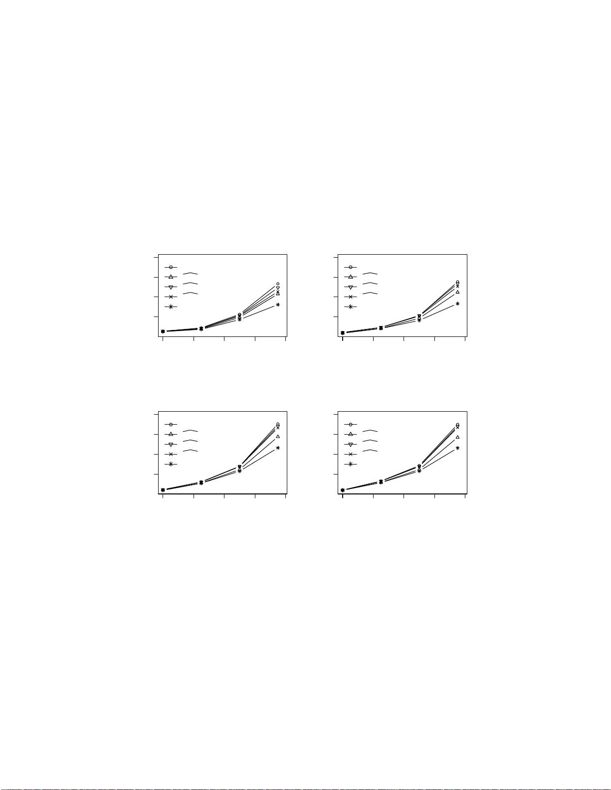
Ev aluating the diagnostic p o w ers of v ariables and their linear com binations when the gol d standard is con tin uous Zhanfeng W ang a,b , Y uan-c hin Iv an Chang b,1 a Dep artment of Statistics and Financ e, University of Scienc e and T e chnolo gy of China, Hefei, 230026, China b A c ademia Sinic a, T aip ei, T aiwan, 11529 Abstract The receiv er op erating c haracteristic (ROC) curv e is a v ery useful to ol for analyzing the diagnostic/classification p ow er of instrumen ts/classification sc hemes a s long as a binar y- scale gold standard is a v a ila ble. When the gold standard is con tin uous and there is no confirmative threshold, ROC curv e b ecomes less useful. Hence, there are sev eral extensions prop osed fo r ev alu- ating the dia g nostic p oten tial of v ariables of in terest. Ho w ev er, due to the computational difficulties of these nonparametric based extensions, they are not easy t o be used for finding the o ptimal com binatio n of v ariables to im- pro v e the individual diagnostic pow er. Therefore, w e prop ose a new measure, whic h extends the AU C index for iden tifying v ariables with go o d p otential to b e used in a diagnostic sc heme. In a dditio n, w e prop ose a threshold gradient descen t based algorithm for finding t he b est linear com bination of v ariables that maximizes this new measure, whic h is applicable ev en when the n umber of v a riables is h uge. Th e estimate of the prop osed index a nd its asymptotic prop erty are studied. The p erformance of the pro p osed metho d is illustrated using b oth syn thesized and real data sets. Keywor d s : R OC curv e, Area under curv e, Gold standard, Classification 1 Corresp o nding a uthor: yc chang@stat.sinica.edu.tw Pr eprint submitte d to Computational St atistic al and D ata Analysi s Novemb er 12, 2021 1. In tr o duction The ROC curv e, founded o n a binary gold standard, is one o f the most imp ortant to ols to measure the diagno stic p ow er of a v ariable or classifier, and its imp ortance has b een in tensiv ely studied by many authors, whic h can easily be fo und in t he lit era t ur e and textb o oks suc h as P ep e (2003) and Krzano wski and Hand (20 0 9). Moreo v er, when the n umber of v ariables is h uge, man y algorithms ha v e b een prop osed for finding the b est com bination of v ariables to increase the individual classification accuracy (Su and Liu (1993), P ep e (2003), Ma and Huang (20 05), and W ang et al. (2007a)). Ho w- ev er, in many classification o r dia gnostic pro blems, the professed binar y gold standard is essen tially deriv ed from a con tin uous-v a lued v ariable. If there is no such confirmativ e threshold for the con tin uous gold standard, then the ev aluation of v aria bles/classifiers according to the R OC curv e based anal- ysis ma y v ary as the c hoices o f thresholds c hange a nd therefore b ecomes less informative. F or example, glycosylated hemoglobin is usually used as a primary diab etic con trol index, and is originally measured as a contin uous- v alued v ariable. Health institutes, suc h a s the W orld Health Organization and National Institutes of Health (NIH), suggest a cutting p oin t fo r it ba sed on current findings fo r diab etic diagnosis and con trol. Once its cutting p oint is fixed, then the asso ciation b et w een the v aria bles of in terests, suc h as new drugs, and this bina r y- scale standard can b e ev aluated using some ROC curv e related analysis metho ds. How eve r, as adv ances are made in science and medicine ab out this disease , this criterion will b e re-ev aluated and re- vised as necessary . Then, t he p erformance ev aluation of v ariables/classifiers ma y v a ry as the binary-reco ding sc heme is c hanged. It is clear that an un w ar- ran ted performance measure may r esult in misle ading conclusions and ma y require re-ev aluation of all the av ailable diagno stic metho ds again ev ery time a new standard is prop o sed. Hence, a measure that directly connects to the con tin uous go ld standard is alw ay s preferred, whic h motiv ates our study of a new measure when the gold standard is con tinuous. Our goal in this pap er is to find a robust measure, whic h is not aff ected by the c hoice of cutting p o int of a g old standard or how the binary outcome is deriv ed from a contin uous gold standard. Although there are a lot of r ep orts ab out the R OC curve, there is still a lac k of study when t he gold standard is not bina r y ( Krzano wski and Hand, 2009). In Henk elman et al. (1990), they prop osed a maxim um likelihoo d metho d under o rdinal scale gold standard. Recen tly , Zho u et al. (2005), 2 Choi et al. (2006), and W ang et al. (2007b) considered the R OC curv e es- timation problems base d on some nonpara metric and Ba y esian approac hes, when there is no gold standard. In addition, some R OC-ty p e analysis with- out a binary gold standard has b een considered in O bucho wski (2005) and Obuc ho wski (2006), where a nonparametric metho d is used to construct a new measure, and man y o t her applications with contin uo us gold standard are discusse d. Ho w ev er, these approa c hes, due to computational issue, are not easy to apply to the case that the optimal com bination of v ariables is of intere st; esp ecially when the n um b er of v ariables is large as in mo dern biological/genetic related studies ( W aik ar et al. (2009)). In this pap er, an extension of the A UC-t yp e measure is prop osed, whic h is indep enden t of the ch oice of threshold of the con tin uous gold standard, and algorithms for fin ding the b est linear com bination of v ariables that maximiz es the prop osed measure ar e studied. Under the join t m ultiv ar iate no rmalit y assumption, the algorithm for the linear com bination can b e founded us- ing the LARS metho d. When this joint normalit y assumption is viola ted, w e prop ose a threshold g radien t descen t ba sed metho d (TGD M) to find the opti- mal linear com bination. Th us, our algorithms also inherit the nice prop erties of LARS and TGDM when dealing with the high dimensional and v a riable selection problems. Numerical studies are conducted to ev aluate the p erfor- mances of the prop osed metho ds with differen t ranges of cutting p oints using b oth syn thesized and real da t a sets. The estimate of this no v el measure and its asymptotic prop erties are also presen ted. In the next section, w e first presen t a no v el measure f o r ev aluating the diagnostic p otential of individual v ariables and then an estimate of this mea- sure. The algo rithms for finding the b est linear comb inatio n are discussed in Section 3. Numerical results based on the syn thesized data and some real examples follow . A summary and conclusions are give n in Section 4. T he tec hnical details are presen ted in App endix. 2. An A UC-t yp e Measure wit h a Con tinuous Gold Standard Before introducing a no v el A UC-ty p e measure based on a con tin uous go ld standard, w e first fix the nota tion and briefly review the definition of the ROC curv e and its related measures. Let Z and Y b e tw o contin uous real- v alued random v ariables, where Z denotes the gold standard and Y is a v ariable of in terest with diagnostic p otential to b e meas ured. Then, fo r example, Z is a primary inde x for measuring a disease and Y is some other measure of 3 sub jects that is related to the disease of in terest. In some medical diagnostics, the primary index is difficult to measure, and w e are usually lo oking for v ariables that a r e strongly asso ciated with Z and easy to measure, to b e used as surrogates. That is wh y w e need to ev a lua te the “lev el of a sso ciation” of Y to Z . Lik ewise, in some bioinformatical studies, in order to dev elop new treatmen ts, w e w ould lik e to identify an y strong asso ciatio ns b et w een some genomic related factors Y to the contin uous g old standard Z . Supp ose that there is an unam biguous thres hold c of Z that can b e used to classify sub jects in to t w o subgroups, and assume further that sub jects with Z > c are classified as diseased, a nd otherwise as mem b ers of the control group. Then the R OC curve, fo r suc h a g iven c , is defined as RO C ( t ) ≡ S D ( S − 1 C ( t )), where S D ( t ) = P ( Y > t | Z > c ) and S C ( t ) = P ( Y > t | Z ≤ c ), and the A UC of v ariable Y is defined as AU C ( c ) = P ( Y + c > Y − c ) (1) where random v ariables Y + c and Y − c resp ectiv ely denote the Y -v alue of sub- jects of the disease and non- disease gro ups with densit y f unctions f ( y | Z > c ) and f ( y | Z < c ). That is, Y + c and Y − c are ra ndom v a r ia bles for the sub- p opulations defined b y { Z > c } and { Z ≤ c } , respectiv ely . It is clear that the AU C ( c ) defined in (1) is a function of c , which will c hange as t he thresh- old c of Z v aries. Hence, when the threshold is dubious, using AU C ( c ) as a measure may misjudge the diagnostic p ow er of Y or the lev el of asso ciatio n b et w een Y and Z . Let f c ( t ) b e a probabilit y densit y function defined on the ra nge of p ossible v alues of c , then AU C I is defined as AU C I ≡ R AU C ( t ) f c ( t ) dt. (2) Hence, by its definition, the prop osed AU C I is indep enden t o f the c hoice o f cutting p oint fo r the contin uo us gold standard, and any monotonic trans- formation of Y as w ell. This kind of threshold indep enden t prop ert y is also one of t he imp o rtan t prop erties of the R OC curv e and AUC when used as measures of diag nostic p erformance. Since AU C I is defined as an integra- tion of AU C ( c ) o v er the range of p ossible cutting p oin ts with resp ect to a w eigh t function f c ( t ), t he supp ort o f f c ( t ) should b e c hosen as a subset of the supp ort of the densit y o f Z . Moreo v er, w e can use f c ( t ) to put differen t w eigh ts on all p o ssible cutting p oin ts of Z if there is some infor ma t io n ab o ut the p ossible cutting p oin t. If Z is an ordinal discrete v ariable, then there are 4 only countable cutting p oin ts, and f c ( t ) can b e c hosen as a pro ba bility mass function of all p ossible cutting p oin ts, a nd the in tegration of (2) b ecomes AU C I = P t i ∈ C AU C ( t i ) f c ( t i ) , (3) where C is a set of all p ossible cutting p oin ts. In particular, when Z is binary , w e can let f c ( t ) b e a degenerated pro babilit y densit y , then AU C I is the same as the original A UC. 2.1. Estimate of AU C I Let random v ariables ( Y i , Z i ) denote a pair of measures fro m sub ject i , for i ≥ 1 . Supp ose that { ( y i , z i ) , i = 1 , . . . , n } are n indep enden t observ ed v alues of random v ariables ( Y i , Z i ), i = 1 , · · · , n . F or a giv en cutting p o in t c , a sub j ect i , i = 1 , . . . , n , is assigned as a “case” if z i > c and o therwise lab eled as a “con trol”. That is, for a giv en c , we divide the observ ed sub jects in to t w o groups; let S 1 ( c ) and S 0 ( c ) b e the case and con trol groups with sample sizes n 1 and n 0 , resp ective ly . It is o b vious that these assignmen ts dep end on the c hoice of c . Then for a fixed c , the em pirical estimate of AU C ( c ) is defined as ˆ A ( c ) = 1 n 0 n 1 X i ∈ S 1 ( c ); j ∈ S 0 ( c ) ψ ( y i − y j ) , (4) where ψ ( u ) = 1, if u > 0; = 0 . 5, if u = 0 and = 0 if u < 0. (It is easy to see that ˆ A ( c ) do es not exist, either c > max { z i , i = 1 , · · · , n } or c < min { z i , i = 1 , · · · , n } , since for these t w o cases, we hav e either n 1 = 0 or n 0 = 0. Therefore, in this pap er, w e assume ˆ A ( c ) = 0 . 5 when either one of the cases o ccurs.) If the whole suppor t of Z is considered as a p ossible range o f cutting p oints , then a natural estimate of AU C I can b e defined as ˆ A I = Z ˆ A ( t ) d ˆ F c ( t ) , (5) where ˆ F c ( t ) is the empirical estimate of the cum ulativ e distribution function of Z based on { z 1 , . . . , z n } . How ev er, in practice, it is ra r e to c ho ose cutting p oints at ranges near the tw o ends of the distribution of Z . Th us, instead o f the whole range of Z , w e migh t explic itly define a w eight function f c ( t ) on a particular critical range. Belo w, w e demonstrate three possible choices : (1) 5 a unif o rm distribution ov er the range of ( − ˆ σ , + ˆ σ ) , where ˆ σ is an empirical standard deviation of Z , sa y f 1 ( t ); (2) a normal densit y with sample mean ˆ µ and standard deviation ˆ σ based on the observ ed v alues o f Z , sa y f 2 ( t ); or (3) using a kerne l densit y estimate, sa y f 3 ( t ), to approximate the marginal densit y of Z . F or differen t w eigh t functions f j ( t ), j = 1 , 2 , 3, the estimate of AU C I is denoted as ˆ A I j = Z ˆ A ( t ) f j ( t ) dt. (6) It is cle ar that o ur method can b e extended to other reasonable c hoices of w eigh t functions. The theorem below states the strongly consiste nt prop erty of ˆ A I j for all j . Theorem 2.1. L et ( Y ∈ R 1 , Z ∈ R 1 ) b e a p air of r andom variables with uni- formly c on tinuous mar gin a l densities. Assume that { ( y 1 , z 1 ) , . . . , ( y n , z n ) } ar e n o bservations of the indep endent a nd i d entic al ly distribute d r and om sam- ple ( Y i , Z i ) , i = 1 , . . . , n . Assume further that Z is the c ontinuous gold stan- dar d. Then for a given f c ( t ) = f j ( t ) , j = 1 , 2 , 3 , wi th pr ob ability one, ˆ A I j − AU C I j → 0 as n → ∞ , wher e ˆ A I j and AU C I j ar e define d as in (6) and(2), r esp e ctively, with c orr esp onding f c ( t ) = f j ( t ) . Pro of of Theorem 2.1 Since b ounded function ˆ A ( c ) con v erges almost surely to AU C ( c ) for all give n c and f c ( t ) is also b ounded densit y function, the pro of of Theorem 2.1 follow s from the dominated con v ergence theorem. It is diffic ult to ha v e an explicit form for the v aria nce of ˆ A I j due to its in tegral form. Th us, a b o otstrap estimate of the v aria nce of ˆ A I j is used and denoted as V ( ˆ A I j ). A similar idea is emplo y ed in Obuc how ski (2006). R ema rk 2.2 . Note that the metho d for calculating (6) ma y dep end on the c hoice of weigh t function. If the empirical densit y of the gold standard is used, then the computation o f it is straigh tforward; if a k ernel densit y of the gold standard is used , then a n umerical in tegrat io n metho d is required. How ev er, in all cases the computation of it are easy since it is an one-dimensional densit y . 3. Linear com bination of v ariables that maximizes AU C I F or a classification or diagnostic problem, there are usually many v ari- ables measured from eac h sub ject, and it is w ell known that a combin atio n 6 of v ariables can usually impro v e on the classification p erformance of a single v ariable. This situation motiv ates us to study ho w to find t he optimal linear com bination of v ariables that maximizes the prop osed measure AU C I . F or classical A UC, Su and Liu (1993) studied the b est linear com bination under a m ultiv ariate normal distribution assumption. Here we extend their idea to AU C I . In addition, w e also a im to address cases with h uge n um b er of v ari- ables, whic h usually inv olve some computational issues and will b e discussed later in this section. 3.1. Optimal Line ar Combination of V ariables Under Joint Normality F or clarit y and conv enience, w e start with a biv a riate normal distribu- tion case, since the linear com bination of v ariables, for a give n v ector of co efficien ts, can be t r eat ed a s a single v a r ia ble. Let U = ( Y , Z ) T b e a random v ector follo wing a biv ariate no r ma l distri- bution with mean v ector µ = ( µ 1 , µ 2 ) T and co v ariance matrix Σ U =  σ 2 1 ρσ 1 σ 2 ρσ 1 σ 2 σ 2 2  . Supp ose that U i = ( Y i , Z i ) T , i = 1 , 2, are t wo indep enden t random v ectors generated from the same distribution of U . Define Q i = exp  − ( U i − µ ) T Σ − 1 U ( U i − µ ) 2  , i = 1 , 2 . Then for a giv en c , pr( Y 1 > Y 2 , Z 1 > c, Z 2 < c ) = Z ∞ −∞ Z y 1 −∞ Z ∞ c Z c −∞ Q 1 Q 2 4 π 2 | Σ U | dz 2 dz 1 dy 2 dy 1 , (7) where | Σ U | denotes the determinan t of matrix Σ U . The conditio nal dis- tribution of Y j giv en Z = z j is a normal distribution with mean ˜ µ j = µ 1 + σ 1 /σ 2 ρ ( z j − µ 2 ) with j = 1 , 2 and v ariance ˜ σ 2 1 = (1 − ρ 2 ) σ 2 1 . Let η ( z 1 , z 2 ) = 1 / (2 π σ 2 2 ) exp( − (( z 1 − µ 2 ) 2 + ( z 2 − µ 2 ) 2 ) / (2 σ 2 2 )). Then, (7) can b e rewritten as pr( Y 1 > Y 2 , Z 1 > c, Z 2 < c ) = Z ∞ c Z c −∞ η ( z 1 , z 2 ) Z ∞ −∞ Z y 1 −∞ 1 2 π ˜ σ 2 1 exp  − ( y 1 − ˜ µ 1 ) 2 + ( y 2 − ˜ µ 2 ) 2 2 ˜ σ 2 1  dy 2 7 dy 1 dz 2 dz 1 = Z ∞ c Z c −∞ η ( z 1 , z 2 )E(Φ( ˜ σ 1 V + ˜ µ 1 − ˜ µ 2 ˜ σ 1 )) dz 2 dz 1 = Z ∞ c Z c −∞ η ( z 1 , z 2 )E(Φ( V + ρ ( z 1 − z 2 ) σ 2 (1 − ρ 2 ) 1 / 2 )) dz 2 dz 1 , (8) where V is a standard normal r a ndom v a riable and Φ is the standard normal cum ulated distribution function. Note that under nor malit y assumption, ρ = 0 implies tha t Y and Z are indep enden t, and it f ollo ws from (8) AU C I = 0 . 5 in this case. No w, supp ose that ˜ X = ( X 1 , . . . , X p ) T is a p - dimensional r andom v ec- tor o f measures of a sub ject, a nd Z is the con tin uous gold standard as b efore. Supp ose l ∈ R p and let Y = l T ˜ X b e a linear com bination of ˜ X . Assum e further that ˜ X fo llo ws a m ultiv a r iate normal dis tribution with mean v ector µ ∗ and co v ar iance matrix Σ. Then Y follo ws a normal dis- tribution with mean µ 1 = l T µ ∗ and v ariance σ 2 1 = l T Σ l . The correla- tion co efficien t b etw een Y and Z is ρ = l T co v ( ˜ X , Z ) / (( l T Σ l ) 1 / 2 σ 2 ), where co v ( ˜ X , Z ) = (cov( X 1 , Z ) , . . . , cov( X p , Z )) T . The n, AU C I for suc h a linear com bination of X i ’s, Y = l T ˜ X , is a function of l : AU C I ( l ) = Z pr( l T ˜ X 1 > l T ˜ X 2 | Z 1 > t, Z 2 < t ) f c ( t ) dt (9) where ( ˜ X T i , Z i ) T , i = 1 , 2, are independen t iden tically distributed samples of ( ˜ X T , Z ) T . Our goal is to find the optimal linear combination o f X 1 , . . . , X p suc h that AU C I is maximized a nd it is known that A UC is scale inv arian t. In order to make the solutio n iden tifiable, we searc h for an l opt suc h that AU C I ( l opt ) ≥ AU C I ( l ) for all p ossible l ∈ R p with k l k = 1. F rom (8 ), ∂ ∂ l E  Φ  V + ρ ( z 1 − z 2 ) σ 2 (1 − ρ 2 ) 1 / 2  = 1 √ 2 exp  − ρ 2 ( z 1 − z 2 ) 2 4 σ 2 2 (1 − ρ 2 )  z 1 − z 2 σ 2 (1 − ρ 2 ) 3 / 2 ∂ ρ ∂ l . (10) Therefore, ∂ AU C I ( l ) ∂ l = ∂ ρ ∂ l Z f c ( t ) Z ∞ t Z t −∞ 1 2 3 / 2 π σ 2 2 exp  − ( z 1 − µ 2 ) 2 + ( z 2 − µ 2 ) 2 2 σ 2 2  exp  − ρ 2 ( z 1 − z 2 ) 2 4 σ 2 2 (1 − ρ 2 )  z 1 − z 2 σ 2 (1 − ρ 2 ) 3 / 2 1 pr( Z 1 > t, Z 2 < t ) dz 2 dz 1 dt = ∂ ρ ∂ l ∆ , (11) 8 where ∆ den tes the in tegratio n par t of the left hand side of (11). Since ∆ > 0, the equation ∂ AU C I ( l ) /∂ l = 0 if and only if ∂ ρ/∂ l = 0; that is, ∂ ∂ l l T co v ( ˜ X , Z ) (( l T Σ l ) 1 / 2 σ 2 ) = 0 . It implies that the optimal linear combination co efficien t l opt = Σ − 1 co v ( ˜ X , Z ) . (12) Note that, as in Su a nd Liu (1993), this optimal linear com bination co effi- cien t l opt is indep enden t of c , and dep ends only on the co v aria nce matr ix of v ariables and the cov ariance b etw een of v ariables and t he g old standard. 3.2. Estimation of the Optimal Line ar Combination Assume tha t { ( ˜ x i , z i ) , i = 1 , · · · , n } is a set of n indep enden t and iden ti- cally distributed random samples, where z i denotes the observ ed go ld stan- dard measures as b efor e, and ˜ x i is its corresp o nding p -dimensional v ector of o bserv ed v aria ble v alues of sub ject i . Without loss of generalit y , we assume that all the comp onen ts of ˜ x and z are cen tralized, since we can alw a ys cen tralize the data by subtracting t heir sample means, a nd define H = ( ˜ x 1 − ¯ x, · · · , ˜ x n − ¯ x ) T as an n × p matrix, a nd ˜ z = ( z 1 − ¯ z , · · · , z n − ¯ z ) T as a v ector of length p , where ¯ x = P n i =1 ˜ x i /n a nd ¯ z = P n i =1 z i /n . Hence, the estimate of l opt based on a sample of size n following from (12) is defined as ˆ l = ( H T H ) − 1 H T ˜ z . (13) Similarly to the linear regression problem, it is clear that ˆ l is a strongly consisten t estimate of l opt under some regularity conditions on ˜ X and Z . Define ˆ A ( c, l ) = 1 n 1 n 0 X i ∈ S 1 ( c ); j ∈ S 0 ( c ) ψ ( l T ˜ x i − l T ˜ x j ) . (14) Then ˆ A I ( l ) = Z ˆ A ( t, l ) f c ( t ) dt (15) is an estimate of AU C I ( l ). It is easy to see that for giv en t , ˆ A ( t, l ) con- v ergenes to ˆ A ( t, l ) uniformly with resp ect to l . Hence, using the dominated con v ergence theorem, it is shown tha t ˆ A I ( ˆ l ) is a strongly consisten t estimate of AU C I ( l opt ) a nd the details are omitted here. This result is stated as a theorem b elo w: 9 Theorem 3.1. S upp ose that the joint distribution of ˜ X ∈ R p , Z ∈ R 1 fol lows a multivariate norma l distribution, wher e Z is the c ontinuous gold standar d, and ˜ X denotes the p -dime nsional ve ctor o f variables. L et { ( ˜ X 1 , Z 1 ) , · · · , ( ˜ X n , Z n ) } b e indep endent and identic a l ly distribute d sa mples of size n . T hen for a giv e n density f c ( t ) , with pr ob ability one, ˆ A I ( ˆ l ) − AU C I ( l opt ) − → 0 , as n → ∞ , wher e AU C I ( l opt ) and ˆ A I ( ˆ l ) ar e defi ne d a s in (9) and (1 5) with l = l opt and ˆ l , r esp e ctively. Equation (13) pro vides a neat solution for the b est linear combination of v aria bles under a joint multiv ariate norma lity assumption. Ho w ev er, it can b e seen f rom (1 3) t ha t the calculation o f ˆ l relies on the computation of an in v erse matrix. Th us, when the n umber of v ar iables is large, the direct calculation o f ˆ l using (13) b ecomes numeric ally unstable. The situation is w orse, when the sample s ize is relativ ely small compared to the n um b er of v ariables. So, we need an alternat ive num erical a pproac h that can handle problems with large p to ov ercome this obstacle. Again, from (13), w e find that the estimate ˆ l can b e view ed as a least square estimate of l in the linear regression mo del b elo w: ˜ z = H l + e, (16) where e is an n -dimensional v ector o f random error. When p is small, then the solution can b e obtained easily a s in regression pro blems. When p is large, then w e can apply the least angle regression shrink age (LARS) metho d (Efron et al., 2 004) t o (16) to obtain an estimate of l . Since this is the same as applying LARS in a regression setup, the prop erties of LARS are therefore inherited. With the assistance of LARS, the prop osed measure can b e applied to ev a luate linear com binations o f lengthy v aria bles. The v ariable selection sc heme will follow f r om L AR S as it is used in regression mo dels. Ho we ve r, when the normality a ssumption is violated or the normal appro ximation to the joint distribution is no t adequate, the empirical results show that the l opt defined in (12) is not a go o d solutio n. Thus , an alternative algo rithm, whic h do es not rely on the normality assumption, is required and dev elop ed b elo w. R ema rk 3.2 . Since t he properties of applying LARS to find the linear com- bination of v ariables a re the same as those in linear regression. W e o mit the details of applying LARS under t he normality assumption. Instead, w e fo cus on the case without a normality assumption. 10 3.3. When the Joint Distribution is Unknown As b efo re, let’s start with a one-dimensional case, and the case with a linear com bination of v ariables will follow easily as a n extension. Similarly to the methods used in Ma and Huang (2005), and W a ng et al. (2007a), w e first use a sigmoid function S ( t ) = 1 / (1 + exp( − t )) to appro x- imate ψ ( · ) in equation (21). Th us, a smo oth estimate of AU C I is defined as ˆ A I s = Z 1 n 1 n 0 X i ∈ S 1 ( t ); j ∈ S 0 ( t ) S  y i − y j h  f c ( t ) dt. (17) It fo llo ws from the results in densit y estimation literature tha t for a suffi- cien tly small windo w width h , S (( y − x ) /h ) ≈ ψ (( y − x ), whic h implies the follo wing asymptotic prop erties of ˆ A I s : Theorem 3.3. Assume that { ( y 1 , z 1 ) , · · · , ( y n , z n ) } ar e n in dep endent and identic al ly dis tribute d samples of ( Y ∈ R 1 , Z ∈ R 1 ) , whe r e Z denotes a c on tinuous g old standar d . D enote the mar ginal densities of Y and Z by f Y and f Z , r esp e ctively. L et F ( z | y ) b e c onditional cumulative function of Z given Y = y . Supp ose that f Y and f Z ar e lar ger than 0 and b ounde d. Assume b oth f Y ( · ) and F ( z |· ) ar e uniformly c o n tinuous. Then for a given pr ob ability density f c ( t ) with h = O ( n − α ) , 1 / 5 < α < 1 / 2 , ˆ A I s − AU C I → 0 almost sur ely as n → ∞ , wher e AU C I and ˆ A I s ar e defi ne d in (2) and (17), r esp e ctively. (The pro of of Theorem 3.3 relies on some classical results of densit y ap- pro ximation theory . The details are given in App endix A.) As b efore, we replace y in (17) with l T ˜ x , then w e ha v e the smo oth estimate of AU C I ( l ) b elow : ˆ A I s ( l ) = Z 1 n 1 n 0 X i ∈ S 1 ( t ); j ∈ S 0 ( t ) S  l T ˜ x i − l T ˜ x j h  f c ( t ) dt. (18) The asymptotic prop erty of ˆ A I s ( l ) follo ws easily fro m Theorem 3.3, a nd is summarized as the follow ing theorem without pro of. 11 Theorem 3.4. S upp ose that { ( ˜ x 1 , z 1 ) , · · · , ( ˜ x n , z n ) } ar e n inde p endent and identic al ly distribute d samples o f ( ˜ X ∈ R p , Z ∈ R 1 ) , w h er e Z denotes the c on tinuous gold standa r d, an d ˜ X is a ve ctor of c orr e s p on d ing variables. L et f c ( t ) b e a pr ob abili ty density. A ssume that for a given c onstant ve ctor l ∈ R p , the c onditions of The or em (3 . 3 ) holds for Y = l T ˜ X and Z . Then fo r h = O ( n − α ) with 1 / 5 < α < 1 / 2 , ˆ A I s ( l ) − AU C I ( l ) → 0 almo s t sur el y as n → ∞ , wher e AU C I ( l ) and ˆ A I s ( l ) ar e defi n e d in (9) and (18), r esp e ctively. R ema rk 3.5 . W e only need to estimate the densit y function of the linear com bination l T ˜ X ∈ R 1 , hence the choic e of h do es not dep end on the length of total v ariables p . Th us, the density estimation part of the prop osed algo rithm will not suffer from the curse of dimensionalit y . F ollo wing Theorem 3.3, w e apply the threshold gradien t desce nt metho d (TGDM) of F riedman and P op escu (200 4) to find the best linear com bina- tion, ˆ l whic h maximizes ˆ A I s ( l ). That is, to find a solution ˆ l = argmax l ˆ A I s ( l ) . (19) F rom equation (1 8 ), we kno w that AU C I s is a lso scale in v a rian t as is AUC. That is, ˆ A I s ( l ) with window width h will equals to ˆ A I s ( k l ) with h = k h fo r a p ositiv e constan t k . Hence, an a nc hor v aria ble is needed suc h that the solution of (19) is unique. TGDM Based Algorithm Let { ( ˜ x 1 , z 1 ) , · · · , ( ˜ x n , z n ) } b e a set of random samples of size n , whic h satisfies the assumption of Theorem 3.4. Define s = ( s 1 , · · · , s p ) T as a p -dimensional v ector with s i = 1 , if the corresp onding empirical AU C I of the i th v ar ia ble is gr eat er than 0 .5 ; o therwise set s i = − 1. Let β i b e a p -dimensional v ector where only the i th comp o nen t equals s i and 0 otherwise. Define R i = ˆ A I s ( β i ), then c ho ose the v ariable with the max i- m um R i v alue as the anchor v ariable. In the following a lgorithm, w e assume that R 1 > R i , for i = 2 , . . . , p without loss of generalit y . Let notation ˆ l i de- note the i th component o f ˆ l , then ˆ l 1 is the coefficien t of the anc hor v ariable. In order to make the co efficien ts iden tifiable, w e set k ˆ l 1 k = 1. F ollo wing the notations defined a b o ve , a TGDM-based a lg orithm for finding the b est linear com bination of v ariables that maximizes AU C I s is stated b elow: Algorithm: 12 (0) Initial stage: Let r = 0 and choose a threshold parameter τ . Set l (0) = ( s 1 , 0 , · · · , 0 ) T . (1) Given l = l ( r ) , calculate the deriv ativ e o f the smo o thed estimate ˆ A I s ( l ) with resp ect to linear co efficien t l , d ( l ( r ) ) = ( d 1 ( l ( r ) ) , · · · , d p ( l ( r ) )) T = ∂ ˆ A I s ( l ) /∂ l | l = l ( r ) . (2) Use the threshold gradien t descen t metho d t o calculate l = l ( r +1) 0 ; that is, l ( r +1) 0 = l ( r ) + δ t ( τ , l ( r ) ) d ( l ( r ) ) for some δ > 0, where t ( τ , l ( r ) ) is an indicator v ector I  d ( l ( r ) ) > τ max { d 1 ( l ( r ) ) , · · · , d p ( l ( r ) ) }  . (3) Find the optimal δ ∗ = argmax δ> 0 ˆ A I s ( l ( r +1) 0 ) with l ( r +1) 0 = l ( r ) + δ t ( τ , l ( r ) ) d ( l ( r ) ), and up date l ( r +1) = l ( r ) + δ ∗ t ( τ , l ( r ) ) d ( l ( r ) ). (4) Rep eat steps (1)-(4) until ˆ A I s ( l ( r +1) ) con v erges. R ema rk 3 .6 . The initial v alue o f l is c hosen as ( s 1 , 0 , · · · , 0) T , since the first comp onen t of l corresponds to the selected anc hor v ariable. In Step (2), w e up date l ( r ) along the direction t ( τ , l ( r ) ) d ( l ( r ) ), where the num b er of nonzero comp onen ts is decided by the threshold parameter τ , and by the definition of t ( τ , l ( r ) ), the lo cations of nonzero comp onen ts of t ( τ , l ( r ) ) are determined by the elemen ts of gradient d ( l ( r ) ). Step (3) is to find a suitable step size δ ∗ along the direction of Step ( 2 ), then up date the linear co efficien ts of v ariables. The criterion of con v ergence of Step (4) has to b e predetermined. (The soft w are used in this pap er (GoldAUC ) is a v aila ble a t h ttp://idv.sinica.edu.t w/ycc hang/soft ware.h tml). 4. Numerical studies In n umerical studies , w e calculate the propo sed measures ˆ A I j , j = 1 , 2 , 3, corresp onding to 3 differen t f c ( t ) as defined b efore. Since the correlatio n co efficien t is a basic statistic to measure the asso ciat io n b etw een t w o con tin- uous v ariables, w e therefore include it in our experimental studies. W e a lso compare the p erformances of our metho ds with that of Obuc how ski’s (20 06) metho d (page 485, Equation (9)) described b elo w: ˆ θ = 1 n ( n − 1) n X i =1 n X j =1 ψ ′ ( y i , z i , y j , z j ) , (20) 13 where i 6 = j , ψ ′ ( y i , z i , y j , z j ) = 1 if y i > y j and z i > z j , o r y i < y j and z i < z j ; = 0 . 5 if y i = y j or z i = z j ; = 0 otherwise . The sample sizes used in our numerical studies are n = 50 and 100 . The window width for the k ernel estimate in ˆ A I 3 is equal to n 1 / 5 . The b o o tstrap sample size for estimating the v ariance of eac h case is 200, and there are 100 replicates for eac h sim ulat io n setup. F or the first exp erimen tal study , the data are generated fro m biv ariate normal distributions with means µ 1 = µ 2 = 1 . 0, standard deviations ( σ 1 , σ 2 ) equal to (1 . 0 , 1 . 0), (1 . 0 , 2 . 0 ), (2 . 0 , 1 . 0 ) and (2 . 0 , 2 . 0), and correlation co efficien ts equal to ρ = 0 . 0, 0 . 25 , 0 . 5, 0 . 75, and 1 . 0. Let ˆ µ and ˆ σ 2 denote t he sample mean and v ariance of z . As in the classical ROC curv e analysis , when a v ariable with no diagnostic p ow er, then its corresp o nding R OC curv e will b e the 45 degree diagonal line of the unit square. If this case holds for all p ossible cutting p o in ts, then it implies t ha t AU C I = 0 . 5. So, we use 0.5 a s the v alue o f the null h yp othesis in our nume rical study . T able 1 shows five statistics fo r differen t sim ulation setups: correlation coefficien t of t w o v ariables ˆ ρ , ˆ A I j , j = 1 , 2 , 3 with corresp onding f c ( t )’s, and ˆ θ from Obucho wski (2006). Figure 1 is a plot of statistics ˆ ρ 2 /V ( ˆ ρ ), ( ˆ A I j − 0 . 5) 2 /V ( ˆ A I j ) for all j ’s, and ( ˆ θ − 0 . 5) 2 /V ( ˆ θ ) v ersus ρ , where V ( ˆ ρ ) and V ( ˆ θ ) are the b o otstrap estimates of v aria nces of ˆ ρ and ˆ θ , resp ectiv ely . When the joint distribution of t w o v ariables follows a biv ariate norma l distribution, the correlation co efficien t is a natural statistic to des crib e the asso ciation b et w een the tw o v ariables. In our study , all five measures increase as the true corr elat io n co efficien t ρ increases, whic h suggests that all measures catc h the linear a sso ciation b et w een v ariable Y and the gold standard Z a s exp ected. In fa ct, ˆ A I j and ˆ θ are v ery close to their t r ue v alues 0.5 and 1.0, when ρ are equal to 0.0 and 1.0, resp ectiv ely . In addition, Fig ure 1 shows that the v a lues of ˆ ρ 2 /V ( ˆ ρ ) and ( ˆ A I j − 0 . 5) 2 /V ( ˆ A I j ), j = 1 , 2 , 3, are lar g er than those of ( ˆ θ − 0 . 5) 2 /V ( ˆ θ ) under curren t sim ulation set up. T a ble 2 shows the results of five measures whe n t here is no association b et w een v aria ble Y and the gold standard Z . That is, the data set used in this table ar e generated fro m the model y = z 2 + ǫ with standard normal error ǫ , where the gold standard z is generated fr o m three differen t distributions: (1) normal distribution, (2) t 2 distribution with free degree 2, and (3) a Cauc h y 14 T able 1: Compar ison of fiv e measur e indexes: ˆ ρ , ˆ A I j , j = 1 , 2 , 3, a nd ˆ θ , where the mar ker and gold standard, ( y , z ), follow multi-v a r iate nor mal distribution with means µ 1 = µ 2 = 1 . 0, with different s tandard deviatio ns σ 1 , σ 2 and distinct co rrela tio n co efficien ts ρ . n ( σ 1 , σ 2 ) Metho d 0.0 0.25 0.5 0.75 1.0 50 (1.0, 1.0) ˆ ρ 0.105(0.076, 0. 140) ∗ 0.252(0.118, 0.130)0.511(0.088, 0.103)0.747(0. 067, 0.064)1.000(0.000, 0.000) ˆ A I 1 0.505(0.064, 0.073) 0.621(0.063, 0.069)0.746(0.053, 0.058)0.866(0.040, 0.038)1.000(0.000, 0.000) ˆ A I 2 0.501(0.065, 0.067) 0.616(0.062, 0.063)0.743(0.046, 0.052)0.856(0.035, 0.033)0.979(0.010, 0.013) ˆ A I 3 0.498(0.065, 0.066) 0.611(0.062, 0.062)0.737(0.045, 0.051)0.846(0.037, 0.034)0.968(0.011, 0.015) ˆ θ 0.504(0.044, 0.049) 0.583(0.044, 0.048)0.673(0.038, 0.044)0.771(0.036, 0.035)1.000(0.000, 0.004) (1.0, 2.0) ˆ ρ 0.106(0.073, 0.136) 0.263(0.118, 0.131)0.477(0.099, 0.109)0.750(0.058, 0.065)1.000(0.000, 0.000) ˆ A I 1 0.497(0.067, 0.073) 0.621(0.061, 0.070)0.730(0.053, 0.061)0.862(0.034, 0.040)1.000(0.000, 0.000) ˆ A I 2 0.495(0.065, 0.066) 0.622(0.061, 0.064)0.729(0.053, 0.054)0.859(0.029, 0.033)0.980(0.008, 0.010) ˆ A I 3 0.496(0.065, 0.066) 0.622(0.062, 0.064)0.729(0.051, 0.054)0.858(0.030, 0.034)0.983(0.004, 0.009) ˆ θ 0.498(0.044, 0.049) 0.583(0.043, 0.049)0.660(0.038, 0.044)0.769(0.032, 0.036)1.000(0.000, 0.004) 100(1.0, 1.0) ˆ ρ 0.085(0.056, 0.098) 0.253(0.083, 0.092)0.497(0.082, 0.075)0.747(0.046, 0.044)1. 000(0.000, 0.000) ˆ A I 1 0.490(0.050, 0.051) 0.620(0.043, 0.048)0.739(0.046, 0.041)0.865(0.024, 0.027)1.000(0.000, 0.000) ˆ A I 2 0.485(0.053, 0.049) 0.622(0.041, 0.046)0.741(0.042, 0.038)0.864(0.023, 0.023)0.987(0.007, 0.008) ˆ A I 3 0.483(0.054, 0.049) 0.620(0.042, 0.045)0.739(0.042, 0.037)0.861(0.024, 0.023)0.982(0.006, 0.009) ˆ θ 0.493(0.033, 0.034) 0.581(0.029, 0.033)0.668(0.033, 0.030)0.771(0.023, 0.024)1.000(0.000, 0.001) (1.0, 2.0) ˆ ρ 0.075(0.057, 0.097) 0.266(0.100, 0.091)0.499(0.081, 0.074)0.739(0.045, 0.046)1.000(0.000, 0.000) ˆ A I 1 0.496(0.049, 0.051) 0.625(0.053, 0.048)0.739(0.042, 0.041)0.859(0.025, 0.027)1.000(0.000, 0.000) ˆ A I 2 0.493(0.050, 0.049) 0.629(0.051, 0.045)0.744(0.041, 0.037)0.862(0.024, 0.023)0.987(0.006, 0.006) ˆ A I 3 0.494(0.049, 0.049) 0.630(0.052, 0.045)0.745(0.041, 0.037)0.862(0.024, 0.024) 0.99(0.003, 0.005) ˆ θ 0.498(0.032, 0.034) 0.586(0.036, 0.033)0.667(0.031, 0.030)0.765(0.022, 0.024)1.000(0.000, 0.001) ∗ Empiric al stand ard deviati ons and mean v alues of bo otstrap standard deviation s are in parentheses. 15 0.0 0.2 0.4 0.6 0.8 5 10 15 20 ( σ 1 , σ 2 )=(2.0,1.0) ρ (n=50) Stat. ρ ^ AUC I1 AUC I2 AUC I3 θ ^ 0.0 0.2 0.4 0.6 0.8 5 10 15 20 ( σ 1 , σ 2 )=(2.0,2.0) ρ (n=50) Stat. ρ ^ AUC I1 AUC I2 AUC I3 θ ^ 0.0 0.2 0.4 0.6 0.8 5 10 15 20 ( σ 1 , σ 2 )=(2.0,1.0) ρ (n=100) Stat. ρ ^ AUC I1 AUC I2 AUC I3 θ ^ 0.0 0.2 0.4 0.6 0.8 5 10 15 20 ( σ 1 , σ 2 )=(2.0,2.0) ρ (n=100) Stat. ρ ^ AUC I1 AUC I2 AUC I3 θ ^ Figure 1: Compariso n o f five measure s: ˆ ρ 2 /V ( ˆ ρ ), ( ˆ A I j − 0 . 5) 2 /V ( ˆ A I j ) , j = 1 , 2 , 3, and ( ˆ θ − 0 . 5) 2 /V ( ˆ θ ), where ( Y , Z ) follow biv a riate nor mal distributions with means µ 1 = µ 2 = 1 . 0, with different s tandard deviatio ns σ 1 , σ 2 and cor relation co e fficient s ρ . 16 distribution. Since z has symmetrical densit y functions for all three cases, it is clear that there is no asso ciat io n b etw een Y and Z . That is, the ideal v alues of the correlation co efficien t estimate | ˆ ρ | , ROC-t yp e indexes estimates | ˆ A I j − 0 . 5 | , j = 1 , 2 , 3 and | ˆ θ − 0 . 5 | should b e close to 0. W e calculate the 25% , 50 % and 75% empirical quan tiles based on 1 0 0 sim ulations. The p - v alues, with a nominal significance lev el equal to 0.05, for statistics ˆ ρ 2 /V ( ˆ ρ ), ( ˆ A I j − 0 . 5 ) 2 /V ( ˆ A I j ), j = 1 , 2 , 3 and ( ˆ θ − 0 . 5) 2 /V ( ˆ θ ) a re also rep orted. It is seen fro m T able 2 that a ll three quan tiles of ˆ A I 3 and ˆ θ are v ery close to 0, while the cor r elation co efficien t seems to o ve r- estimate the asso ciatio n of Y and Z in this experimen t. When the tail of the distribution of Z b ecomes hea vier, the quantile s a nd p -v alues of ˆ ρ b ecome further from 0.0 and nominal 0.05, resp ectiv ely . Esp ecially , when Z is from a Cauc h y distribution, the 25% quan tiles are larger than 0.5 and the corresp onding p -v alues are g reater than 0.3. The p erformances of ˆ A I 3 and ˆ θ are b etter than those of ˆ A I 1 and ˆ A I 2 when Z is not fro m a normal distribution. This is b ecause ˆ A I 3 is based on a k ernel estimate of f c ( t ) and ˆ θ is founded on a nonparametric metho d, they are not affected by the distribution of Z , and therefore v ery stable ev en wh en Z is not normally distributed. As a summarization and conclusion to the results of F igure 1, and T ables 1 and 2, b oth ˆ A I 3 and ˆ θ are recommended fo r detecting the asso ciation b etw een v ariables and the con tin uous gold standard. Although ˆ θ is considered as a natural extension of the ordinary AUC index, it is w ort h noting that the p erformance of ˆ A I j (esp ecially ˆ A I 3 ), in these cases , are are ve ry comp etitiv e. 4.1. Combin ation of V ariables Both cor r elation co efficien t (CC) and the TGDM algorithm are used to obtain the optimal linear combinations of v ariables. W e then calculate ˆ A I 3 and ˆ θ o f the corresponding combination of v ariables based on the coefficien t v ectors obtained from these t wo metho ds. The threshold parameter τ in the TGDM algorithm is equal to 1.0 in our studies. The data set are generated from Z = l T ˜ X + ǫ , where ˜ X follows a p dimensional m ultiv ariate normal distribution with mean v ector (0 , . . . , 0 ) T and a n iden tit y co v ariance matrix, and the true l = (1 . 0 , 1 . 0 , 0 . 0 , · · · , 0 . 0) T . Error term ǫ is generated from either the standard normal distribution or a Cauc hy distribution. In this exp eri- men tal study , w e ha v e tried three differen t dimensions of X ( p = 4 , 10 , 20) for all cases, and o nly v ariables x 1 and x 2 ha v e non-zero coefficien ts. That is, only these t wo v ariables are asso ciated with the gold standard. Moreo v er, 17 T able 2: Compa r ison of different metho ds when there is no asso cia tion b etw een v ariable Y and the g o ld standard Z . The data set ( y , z ) is ge nerated fro m mo del y = z 2 + ǫ with standar d norma l error ǫ . Three different distributions of z are used, which are a nor mal distribution, a t 2 distribution with free degree 2 and a Cauch y distribution. Normal t 2 Cauc hy n Mo del (25% , 50% , 75%) p-v alue ∗ (25% , 50% , 75%) p-val ue (25% , 50% , 75%) p-v alue 50 ˆ ρ (0.086, 0.175, 0.287) 0.13 (0.277, 0.544, 0.802) 0.30 (0.515, 0.834, 0.948) 0.33 ˆ A I 1 (0.031, 0.060, 0.110) 0.09 (0.048, 0.079, 0.125) 0.12 (0.044, 0.074, 0.125) 0.13 ˆ A I 2 (0.025, 0.054, 0.090) 0.06 (0.041, 0.076, 0.120) 0.13 (0.040, 0.078, 0.150) 0.15 ˆ A I 3 (0.022, 0.050, 0.087) 0.06 (0.036, 0.060, 0.090) 0.09 (0.028, 0.055, 0.088) 0.09 ˆ θ (0.021, 0.043, 0.081) 0.08 (0.034, 0.060, 0.087) 0.09 (0.025, 0.049, 0.090) 0.08 100 ˆ ρ (0.055, 0.114, 0.202) 0.07 (0.305, 0.527, 0.728) 0.2 7 (0.603, 0.825, 0.931) 0.37 ˆ A I 1 (0.022, 0.044, 0.072) 0.07 (0.016, 0.035, 0.072) 0.06 (0.029, 0.052, 0.098) 0.15 ˆ A I 2 (0.020, 0.033, 0.059) 0.06 (0.014, 0.033, 0.064) 0.05 (0.026, 0.048, 0.096) 0.14 ˆ A I 3 (0.017, 0.034, 0.060) 0.06 (0.009, 0.032, 0.056) 0.04 (0.018, 0.041, 0.07) 0.08 ˆ θ (0.015, 0.032, 0.049) 0.07 (0.012, 0.031, 0.054) 0.04 (0.014, 0.036, 0.065) 0.06 ∗ Nominal significance level is 0.05. a sof tw are based on t he TGDM alg o rithm to calculate the optimal linear com bination of v ariables is a v ailable a s an R pack age. It is also w ort h noting that there is no algorithm or discu ssion in Obuc how ski ( 2 005) ab out finding the linear com bination o f v ariables based on ˆ θ . T a ble 3 lists the v alues of ˆ A I 3 and ˆ θ for individual v ariables, x 1 and x 2 , and the linear com binations based on the CC and TGDM methods. F rom this table, w e find that ˆ A I 3 and ˆ θ for linear combinations o f v ariables a r e alw a ys larg er than for individual v aria bles, whic h confirms that linear com- binations of v ariables can improv e on the the diagnostic p ow er of individual v ariables. When ǫ follo ws the standard normal distribution, ˆ A I 3 and ˆ θ for linear com binations based on b oth TGDM and CC are v ery close. How eve r, when ǫ is a Cauc h y distribution, the TGDM metho d has larger ˆ A I 3 and ˆ θ than com binations based on CC. This is b ecause the CC metho d relies on the normality assumption, while TGDM do es not. In addition, from T able 3, w e can see that ˆ A I 3 is larger than ˆ θ . In most of the cases, the s tanda r d deviations of TGD M are smaller tha n those of ˆ θ , whic h suggests that the lin- ear com binations based o n TGDM hav e greater diagnostic p ow er, although the difference ma y not b e statistically significan t in our sim ulation. 18 T able 3: Results of linea r combination us ing cor relation co efficient (CC) and TGDM metho d. N onz er o coef . + Distribution p ∗∗ n Metho d x 1 x 2 CC TGDM N or mal 4 50 ˆ A I 3 0.773(0.0 54) ∗ 0.786(0.0 52) 0.900(0.024) 0.900(0.028) ˆ θ 0.694(0.0 43) 0.702(0.042) 0.815(0. 028) 0.815(0.03 1) 100 ˆ A I 3 0.782(0.0 33) 0.785(0.035) 0.904(0. 018) 0.906(0.01 8) ˆ θ 0.693(0.0 27) 0.696(0.030) 0.807(0. 021) 0.809(0.02 1) 10 50 ˆ A I 3 0.785(0.0 48) 0.773(0.046) 0.909(0. 021) 0.900(0.03 1) ˆ θ 0.703(0.0 37) 0.692(0.040) 0.824(0. 027) 0.815(0.03 3) 100 ˆ A I 3 0.791(0.0 36) 0.789(0.032) 0.913(0. 015) 0.913(0.01 6) ˆ θ 0.699(0.0 30) 0.700(0.025) 0.818(0. 019) 0.817(0.02 0) 20 50 ˆ A I 3 0.767(0.0 51) 0.779(0.053) 0.928(0. 018) 0.897(0.03 4) ˆ θ 0.689(0.0 42) 0.698(0.042) 0.852(0. 026) 0.813(0.03 9) 100 ˆ A I 3 0.782(0.0 33) 0.783(0.032) 0.922(0. 015) 0.915(0.01 6) ˆ θ 0.693(0.0 28) 0.696(0.025) 0.828(0. 019) 0.820(0.01 9) C auchy 4 50 ˆ A I 3 0.659(0.0 67) 0.640(0.068) 0.669(0. 107) 0.735(0.07 3) ˆ θ 0.629(0.0 46) 0.614(0.046) 0.619(0. 088) 0.685(0.05 9) 100 ˆ A I 3 0.660(0.0 56) 0.657(0.047) 0.659(0. 094) 0.724(0.07 7) ˆ θ 0.629(0.0 36) 0.625(0.032) 0.615(0. 078) 0.679(0.06 3) 10 50 ˆ A I 3 0.648(0.0 64) 0.645(0.072) 0.690(0. 099) 0.750(0.06 7) ˆ θ 0.620(0.0 45) 0.618(0.048) 0.628(0. 079) 0.689(0.05 6) 100 ˆ A I 3 0.648(0.0 83) 0.638(0.082) 0.664(0. 104) 0.733(0.10 1) ˆ θ 0.625(0.0 33) 0.618(0.035) 0.614(0. 063) 0.683(0.06 1) 20 50 ˆ A I 3 0.647(0.0 93) 0.657(0.096) 0.740(0. 123) 0.789(0.09 6) ˆ θ 0.623(0.0 44) 0.628(0.046) 0.665(0. 083) 0.719(0.05 2) 100 ˆ A I 3 0.634(0.1 23) 0.638(0.120) 0.649(0. 142) 0.739(0.14 7) ˆ θ 0.624(0.0 32) 0.627(0.029) 0.604(0. 068) 0.689(0.06 9) + N onz er o coef . represents v ariables with n on - zero co efficients in tru e mo del. ∗ Empirical standard deviations are in paren theses. ∗∗ p denotes num b er of t otal v ariables in true mo del and the num b er of non-zero v ariables is p 1 = 2. 19 4.2. R e al exam ples W e apply the prop osed measures to three real data sets : tumor, prostate and diab etes da t a sets, whic h are used in Obuch owsk i ( 2 005), Stamey et al. (1989) a nd Willems et a l. (1 9 97), resp ectiv ely . In the tumor data set, there are 74 patien ts and only tw o surgery v ar ia bles: the computed to mo g raph y (CT) and a fictitious test (Fi). The contin uous gold standard of this data set is the s ize of the renal tumor mass. The prostate data has 9 7 patien ts with prostate specific an tigen as its gold standard together with 6 contin u- ous v ariables, whic h are cancer v olume, prostate weigh t, age (Age), b enign prostatic h yp erplasia amoun t, capsular p enetration, and p ercen tage G leason scores 4 or 5 (Pgg45). Except v ariables Age and Pgg45, the others are re- co ded in log-scale and denoted b y Lcav o l, Lwe ight, Lbph, Lcp and Lpsa, accordingly . The original diab etes data consists of 403 sub jects, but we fol- lo ws Willems et al. (1997) to delete 22 sub jects with missing v ariables. Of the remaining 381 sub jects from this data set used in our n umerical study , 222 are females and 159 are males. The following 8 contin uo us v aria bles are used in this data set: total c holesterol (Chol), stabilized g lucose (Stab.glu), high densit y lip oprotein (Hdl), c holesterol/HDL ra tio (Ratio), age (Age), b o dy mass index (BMI) and w aist/hip ratio (WHR). The gold standard for this data set is glycosylated hemoglobin (Glyhb), whic h is commonly used as a measure of the pro g ress of diab etes. In addition to analyzing the en tire diab etes dat a set, w e also inv estigate female and male subgroups, separately . W e normalize the data b efore applying the prop osed measures to each data set to a v oid scale v a riations. T able 4 presnets ˆ A I 3 and ˆ θ for individual v ariables with p -v alue less tha n 10 − 7 . F rom T able 4, w e find that ˆ A I 3 selects more v aria bles than ˆ θ for some cases. Note tha t ˆ A I 3 are m uc h larger than ˆ θ with comp etitiv e standar d deviations in these cases. T a ble 5 lists the linear co efficien ts obtained using the TGDM and CC metho ds, and their corr esp onding ˆ A I 3 and ˆ θ v alues for all data sets, including the male and female subgroups of the diab etes dat a set. In the tumor data set, Fi ha s a larg er ˆ A I 3 v alue than CT; that is, Fi has a gr eat er asso ciation with the size of the renal tumor mass f o r tumor data. In the pro stat e data set, Lca v ol has the largest ˆ A I 3 v alue; that is, Lcav ol is most highly asso ciat ed with prostate sp ecific an tigen among all v ariables considered in the prostate data set. F or the diab etes data set and its male and female subgroups, the largest ˆ A I 3 and the v ariable with the largest co efficien t v alue is Stab.glu; that is , Stab.glu has the highest p oten tial to diagnose diabetes in terms of glycosylated hemoglobin index. As exp ected, from T ables 4 and 5, the linear 20 T able 4: Results of ROC measure index es: ˆ A I 3 and ˆ θ , of single markers for tumor, pro state, diabe tes , diab etes-female a nd diab etes-ma le data sets. T umor Data Method CT Fi T umor ˆ A I 3 0.943(0.0 14) ∗ 0.982(0.0 11) ˆ θ 0.871(0.0 20) 0.956(0.0 08) Prostate Data Method Lca vol Lw eight Lcp Pgg45 Prostate ˆ A I 3 0.865(0.0 22) 0.722(0.0 34) 0.759(0.035) 0.744(0. 035) ˆ θ 0.758(0.0 27) 0.647(0.0 27) 0.675(0.031) 0.676(0. 028) Diab et es Data Metho d Chol Stab.glu Ratio Age Diab et es ˆ A I 3 - 0.779(0.0 21) 0.662 (0.022) 0.711(0.019) ˆ θ - 0.687(0.0 17) 0.600 (0.015) 0.644(0.014) Diab et es- ˆ A I 3 0.667(0.0 29) 0.78 6(0.022) - 0.732(0.0 25) female ˆ θ - 0.691(0.0 21) - 0.665(0.019) Diab et es- ˆ A I 3 - 0.769(0.0 39) 0.689 (0.034) 0.681(0.030) male ˆ θ - 0.682(0.0 30) - - ∗ Bootstrap standard d eviation is in parentheses. com binations based on TGD M and CC usually hav e larg er ˆ A I 3 and ˆ θ v alues than individual v ariables do, and similarly , ˆ A I 3 and ˆ θ v alues for combinations from TGDM are a little bit larger than those obtained using the CC metho d. In real data sets the relation is seldom linear, whic h is the reason wh y the com binations o bta ined using TGDM p erform b etter than others. 5. Conclusion and Discussion In this pap er, w e first prop ose a new measure for ev aluating the p oten- tial diagnostic p ow er o f individual v ariables, when there is only a con tinuous 21 T able 5: Results of optimal linea r co efficients and corres p o nding ROC measure indexes: ˆ A I 3 and ˆ θ , for tumor, pr ostate, diab etes, diab etes-female and diab etes -male data sets. T umor Data Method Coef. ROC-t ype indexes CT Fi ˆ A I 3 ˆ θ T umor CC -0.118 1.076 0.981(0.011) 0.950(0.009) TGDM 0.044 1.000 0.983 (0.011) 0.957(0.008) Prostate Data Method Coef. R OC-type indexes Lca vol Lw eight Age Lbph Lcp Pgg45 ˆ A I 3 ˆ θ Prostate CC 0.642 0.214 -0.118 0.099 0.017 0.147 0.892(0.018) 0.791(0.024) TGDM 1.000 0.264 -0.108 0.135 -0.013 0.189 0.891(0.017) 0.789(0.023) Diab etes Data Method Coef. ROC-t ype i ndexes Chol Stab.glu Hdl Ratio Age BMI WHR ˆ A I 3 ˆ θ Diab etes CC 0.074 0.668 0.018 0.101 0.101 0.017 0.019 0.816(0.017) 0. 717(0.015) TGDM 0.061 1.000 -0.027 0.099 0.373 0.140 0.011 0.82 6(0.018) 0.723(0.016) Diab etes-female CC 0.109 0.659 -0.073 0.027 0.106 0.029 0.069 0.834(0.021 ) 0.737(0.019) TGDM 0.253 1.000 -0.164 -0.007 0.389 0.133 0. 199 0.842(0.019) 0.741(0.018) Diab etes-male CC -0.005 0.701 0.141 0. 243 0.085 - 0.049 -0.002 0.786(0.03) 0.691(0.025) TGDM -0.016 1. 000 0.009 0.179 0.367 0.100 -0. 040 0.811(0.031) 0.706(0 .027) ∗ ROC-t ype indexes used here are AU C I 3 and ˆ θ . 22 gold standard a v ailable and no confirmativ e threshold for it is kno wn. The prop osed measure is an AUC-t ype index that shares the threshold indep en- den t prop ert y of the ROC curv e and A UC, and can also b e used to ev aluate the p erformance o f classifiers when the gold standard v ariable is essen tially con tin uous, and the threshold is con trov ertible. Numerical results sho w that the prop osed nov el index is v ery comp etitive to the existence metho d. In addition, w e prop ose algorithms, based on t he newly defined index, for finding the b est linear com bina t io n of v a riables, whic h is useful f rom a prac- tical pro sp ect when there are m ultiple v ariables considered at a time, and ho w to ev aluate or select a go o d com bination o f v ariables is an imp ortant issue. Here w e also study n umerical metho ds f o r finding the linear com bina- tion of v aria bles t hat maximizes the prop osed measure. When the normality assumption of v ariables is v alid, the b est linear com bination solution can b e realized as a solution to a linear system . Th us, under an assumption of no r- malit y and when the n um b er of v ariable p is large, the L AR S algo rithm can b e applied to o btain suc h a linear com binat io n. This also implies tha t the LARS-t yp e v aria ble selection sc heme can b e conducted ev en when no binary- scale g old standard is av ailable. When the joint distribution of v ar ia bles is unkno wn, the pro p osed measure is then approximated using a nonparametric k ernel densit y estimation metho d. In this case, w e prop osed a TGD M-based algorithm to calculate the b est linear com bination of v ariables. Based on n umerical results, w e f ound t ha t o ur metho d is n umerically stable with com- putational adv an tage when there are large num b er of v a riables considered and combination of v ariables is of in terest. Moreo v er, our metho d can b e easily extended to an ordinal-scale gold standard with a suitable c hoice of a w eigh t function for cutting p oints, whic h will b e rep ort ed elsewhere. App endix Let random v ariables ( Y i , Z i ) denote a pair of measures fro m sub ject i , for i ≥ 1 . Supp ose that { ( y i , z i ) , i = 1 , . . . , n } are n indep enden t observ ed v alues of random v ariables ( Y i , Z i ), i = 1 , · · · , n . F or a giv en cutting po in t c , a sub ject i , i = 1 , . . . , n , is assigned as a “case” if z i > c a nd otherwise lab eled as a “ con trol”. That is, for a g iv en c , w e divide the o bserv ed sub jects in to tw o groups; let S 1 ( c ) and S 0 ( c ) b e the case and con trol groups with sample sizes n 1 and n 0 , resp ectiv ely . Then we prop o se a nat ura l estimate of A UC index, AU C I , with con tinu- 23 ous gold standard, ˆ A I = Z ˆ A ( t ) d ˆ F c ( t ) , (21) where ˆ A ( c ) is defined as ˆ A ( c ) = 1 n 0 n 1 X i ∈ S 1 ( c ); j ∈ S 0 ( c ) ψ ( y i − y j ) , ψ ( u ) = 1, if u > 0; = 0 . 5, if u = 0 and = 0 if u < 0 and ˆ F c ( t ) is the empirical estimate of the cum ulative distribution function of Z based on { z 1 , . . . , z n } . Ho w ev er, in practice, it is rare to choose cutting p oin ts at ranges near the t w o ends of the distribution of Z . Thus , instead of the whole r ange o f Z , w e migh t explicitly define a w eigh t function f c ( t ) on a particular critical r ange. Since the step function ψ ( · ) in (21) is not con t inuously differen t ia ble, a smo oth estimate of AU C I is defined as ˆ A I s = Z 1 n 1 n 0 X i ∈ S 1 ( t ); j ∈ S 0 ( t ) S  y i − y j h  f c ( t ) dt, (22) where S ( t ) is a sigmoid function 1 / (1 + exp( − t )) and h is window width. App endix A: P ro of of Strong Consistency of ˆ A I s ( l ) The pro of of the strong consistency of smo othed AU C I ( l ) estimator ˆ A I s ( l ) follo ws from the following three lemmas. Lemma 5.1. Supp ose that X 1 , · · · , X n is a se quenc e of indep endent and iden- tic al ly d i stribute d r andom v ariables with values in R 1 , and a uniformly c ontin- uous density f ( · ) . L et k ( x ) b e a b o und e d pr ob abil i ty density an d the Dirichlet series P ∞ n =1 n exp( − γ η n ) , η n = n h 2 c on v e r ges for any γ > 0 . Then Z ∞ −∞ | f n ( x ) − f ( x ) | dx → 0 , al most sur ely as n → ∞ , wher e f n ( x ) = 1 n h P n i =1 k (( x − X i ) /h ) is a k e rnel d e n sity estimator of f ( x ) . (The pro of of Lemma 5.1 can b e found in Nadara ya (1989), Theorem 3.1, page 55. So , it is omitted here.) 24 Lemma 5.2. Supp ose that X 1 , · · · , X n is a se quenc e of indep endent and iden- tic al ly distribute d r andom variab les with values in R 1 , and a unif o rmly c on- tinuous density. Then with pr ob ability one, as n → ∞ sup x ∈ R 1 | F n ( x ) − F ( x ) | → 0 , wher e F n ( · ) and F ( · ) ar e the empiri c al distribution and distribution functions of X , r esp e ctively. Pro of of Lemma 5.2: F rom Nada ra y a (1989) (Equation (1.4), page 43), w e ha v e pr( sup x ∈ R 1 | F n ( x ) − F ( x ) | > η n − 1 / 2 ) ≤ c exp ( − 2 η 2 ) , (23) whic h completes the pro of of Lemma 5.2. Lemma 5.3. Assume that { ( y 1 , z 1 ) , · · · , ( y n , z n ) } ar e n indep e n dent and identic al ly dis tribute d samples of ( Y ∈ R 1 , Z ∈ R 1 ) , whe r e Z denotes a c on tinuous gold stand ar d. F or a given c , let ˜ f ( y | Z > c ) b e a c onditiona l density f unction o f Y given Z > c . Supp ose that c o nditions of T h e or em 3 holds. The n ˜ f ( ·| Z > c ) is unif o rm ly c ontinuous. Pro of of Lemma 5.3: By the Ba y esian theorem, w e hav e ˜ f ( y | Z > c ) = R ∞ c f ( y , z ) dz pr( Z > c ) . (24) F or a n y y i ∈ R 1 , i = 1 , 2, R ∞ c f ( y 1 , z ) dz − R ∞ c f ( y 2 , z ) dz = R ∞ c [ f ( z | y 1 ) f Y ( y 1 ) − f ( z | y 1 ) f Y ( y 2 )] dz + R ∞ c [ f ( z | y 1 ) f Y ( y 2 ) − f ( z | y 2 ) f Y ( y 2 )] dz = [ f Y ( y 1 ) − f Y ( y 2 )][1 − F ( c | y 1 )] + [ F ( z | y 2 ) − F ( z | y 1 )] f Y ( y 2 ) , (25) where f ( z | y ) is a conditional densit y function o f Z giv en Y = y and f Y ( y ) is a densit y function of mark er Y . F rom the conditions of Theorem 3, w e ha v e b ≡ pr( Z > c ) > 0, f Y ( · ) < M and b oth f Y ( · ) and F ( z | · ) − F ( z |· ) are uniformly con tin uous. Hence, for any ǫ > 0 , there exists a δ > 0, for any y 1 and y 2 satisfying | y 1 − y 2 | < δ , w e hav e | f Y ( y 1 ) − f Y ( y 2 ) | < bǫ/ 2 | F ( z | y 2 ) − F ( z | y 1 ) | < bǫ/ (2 M ) . (26) 25 Consequen tly , b y (24) , (25 ) and (26) w e get that for a give n c , | ˜ f ( y 1 | Z > c ) − ˜ f ( y 2 | Z > c ) | < 1 b {| f Y ( y 1 ) − f Y ( y 2 ) | (1 − F ( c | y 1 )) + | F ( z | y 2 ) − F ( z | y 1 ) | f Y ( y 2 ) } < ǫ/ 2 + ǫ/ 2 = ǫ. (27) It follo ws that ˜ f ( ·| Z > c ) is uniformly con tinuous . Pro of of Theorem 3: By the triangle inequalit y , w e hav e, for fixed l ,    ˆ A I s − AU C I    ≤    ˆ A I s − ˆ A I    +    ˆ A I − AU C I    = ( I ) + ( I I ) (say) . (28) F rom Theorem 1, (I I) con v erges to 0 almost surely as n go es to ∞ ; that is ˆ A I − AU C I → 0 almost surely as n → ∞ . (29) F rom (2 1) and (17), ( I ) =    R 1 n 1 n 0 P i ∈ S 1 ( t ); j ∈ S 0 ( t ) S  y i − y j h  f c ( t ) dt − R 1 n 1 n 0 P i ∈ S 1 ( t ); j ∈ S 0 ( t ) ψ ( y i − y j ) f c ( t ) dt    ≤ R    1 n 1 n 0 P i ∈ S 1 ( t ); j ∈ S 0 ( t ) S  y i − y j h  − 1 n 1 n 0 P i ∈ S 1 ( t ); j ∈ S 0 ( t ) ψ ( y i − y j )    f c ( t ) dt. Due to n 1 + n 0 = n , then at least one o f n 1 → ∞ and n 0 → ∞ holds as n tends to ∞ . Without loss of generalit y , assume that n 1 tends to ∞ . Then ( I ) ≤ R 1 n 0 P j ∈ S 0 ( t )    1 n 1 P i ∈ S 1 ( t ) S  y i − y j h  − ˜ F ( y j | Z > t )    f c ( t ) dt + R 1 n 0 P j ∈ S 0 ( t )    1 n 1 P i ∈ S 1 ( t ) ψ ( y i − y j ) − ˜ F ( y j | Z > t )    f c ( t ) dt, (30 ) where ˜ F ( ·| Z > t ) is the conditional cum ulativ e distribution f unction of Y giv en { Z > t } . Let ˜ f ( ·| Z > t ) b e its conditional densit y function. By Lemma 5.3, ˜ f ( ·| Z > t ) is uniformly contin uous. Let h = n − α , 1 / 5 < α < 1 / 2. Set η n = nh 2 = n 1 − 2 α , and the Diric hlet series P ∞ n =1 n exp( − γ η n ) con v erges f or an y γ > 0. Th us, the conditions o f Lemma 5.1 are satisfied. Let k ( t ) denote the deriv ativ e of S ( t ), then k ( t ) is 26 a b ounded probability densit y . Thu s, b y Lemma 5.1 , sup y ∈ R 1    1 n 1 P i ∈ S 1 ( t ) S  y i − y h  − ˜ F ( y | Z > t )    = sup y ∈ R 1    R y −∞  1 n 1 h P i ∈ S 1 ( t ) k  y i − t h  − ˜ f ( t | Z > t )  dt    ≤ R ∞ −∞     1 n 1 h P i ∈ S 1 ( t ) k  y i − t h  − ˜ f ( t | Z > t )     dt − → 0 , almost surely as n → ∞ . (31) F rom Lemma 5 .2, w e hav e sup y ∈ R 1       1 n 1 X i ∈ S 1 ( t ) ψ ( y i − y ) − ˜ F ( y | Z > t )       − → 0 , almost surely as n → ∞ . (32) F rom (3 0), (31) and (32), w e prov e that ˆ A I s − ˆ A I → 0 , almost surely as n → ∞ . (33) Put (29) and (33) together to complete the pro of of Theorem 3. Ac knowle dgemen ts This work is part ia lly supp orted via NSC97-2118- M-001-00 4-MY2 funded b y the National Science Council, T a ip ei, T aiw a n, R OC. References Choi, Y., Johnson, W., Collins, M., Gardner, I. (2006). Bay esian infer- ences for receiv er operat ing c haracteristic curv es in the absence of a go ld standard. Journal of A gricutur e, Bio lo g i c al a n d Envir omental Statistics 11 , 210 – 229. Efron, B., Johnstone, I., Hastie, T., Tibshirani, R. (2004). Least ang le regression. Ann. Statist. 32 , 407– 4 99. F riedman, J. H., Popescu, B. E. (2004). Gra dient directed regular izat io n fo r linear regression and classification. T ec h. rep., Departmen t o f Statistics, Stanford Univ ersit y . Henk elman, R., Ka y , I., Bronskill, M. (19 90). Receiv er operating c harac- teristic analysis without truth. Me dic al De cis i o n Making 10 . 27 Krzano wski, W., Hand, D. (2009) . R OC curves for Continuous Data . CR C Press, London. Ma, S., Huang, J. ( 2005). Regularized ro c metho d for disease classification and biomark er selec tion with microarra y data. Bioinfo rmatics 21 , 4356– 4362. W a ik ar, S., Betensky , R., , Bo n v en tre, J. (2009) . Creatinine as the gold standard for kidney injury biomark er studies? Neph r ol Dial T r ansp l a nt 24 , 3263–3 2 65. Nadara ya, E. A. (19 89). Nonp ar ametric Estimation of Pr o b ability D e nsities and R e gr ession Curves . Kluw er Academic. Obuc ho wski, N. (2005 ) . Estimating and comparing diagno stic tests’ accuracy when the gold standard is not binary . Statistcs in Me dicine 20 , 3 261–3278 . Obuc ho wski, N. (2006). An ro c-type me asure of diag nostic accuracy when the gold standard is contin uo us-scale. Statistcs in Me dicine 25 , 481–493 . P ep e, M. (2003). The Statistic al Rvaluation of Me dic al T ests for Classific a- tion and Pr e diction . Unive rsity Press, Oxford. P ep e, M, Thompson, M. (2000). Comb ining diagno stic test results to in- crease accuracy . Biostatistics 1 , 123–140. Pfeiffer, R., Castle, P . (2005). With o r without a goldstandard. Epidemiolo gy 16 , . Stamey , T., Kabalin, J., McNeal, J., Johnstone, I., F reiha, F., Redwine, E., Y ang, N. (1989). Prostate sp ecific antigen in the diagnosis and treat- men t of adeno carcinoma of the prostate: Ii. radical prostatectom y treated patien ts. Journa l of Ur olo gy 141 , 107 6–1083. Su, J., Liu, J. (1993). Linear com binations of m ultiple diagnostic markers . J. A m. Statist. Ass. 88 , 1350– 1355. W a ng, Z., Chang, Y., Ying, Z ., Zhu, L., Y ang, Y. ( 2007a). A parsimonious threshold-indep enden t protein feature selection me tho d t hrough the area under receiv er op erating c haracteristic curv e. Bioinform atics 23 , 278 8– 2794. 28 W a ng, C ., T urn bull, B., Gr¨ ohn, Y., Nielsen, S. (2007b). Nonparametric estimation of ro c curv es based on ba y esian mo dels when the true disease state is unkno wn. Journal of A gricultur e, Bio l o gic al and Envir omental Statistics 12 . Willems, J., Sa unders, J., Hunt, D., Sc horling, J. (1997). Prev alence of coronary heart disease risk factors among rur a l blac ks: A communit y- ba sed study . Southern Me dic al Journal 90 , 814 –820. Zhou, X.-H., Castelluc cio, P ., Z ho u, C. (2005). Nonparametric estimation of ro c curv es in the absence of a gold standard. Biom etrics 61 , 600–60 9. 29