Iterative Reweighted Algorithms for Sparse Signal Recovery with Temporally Correlated Source Vectors

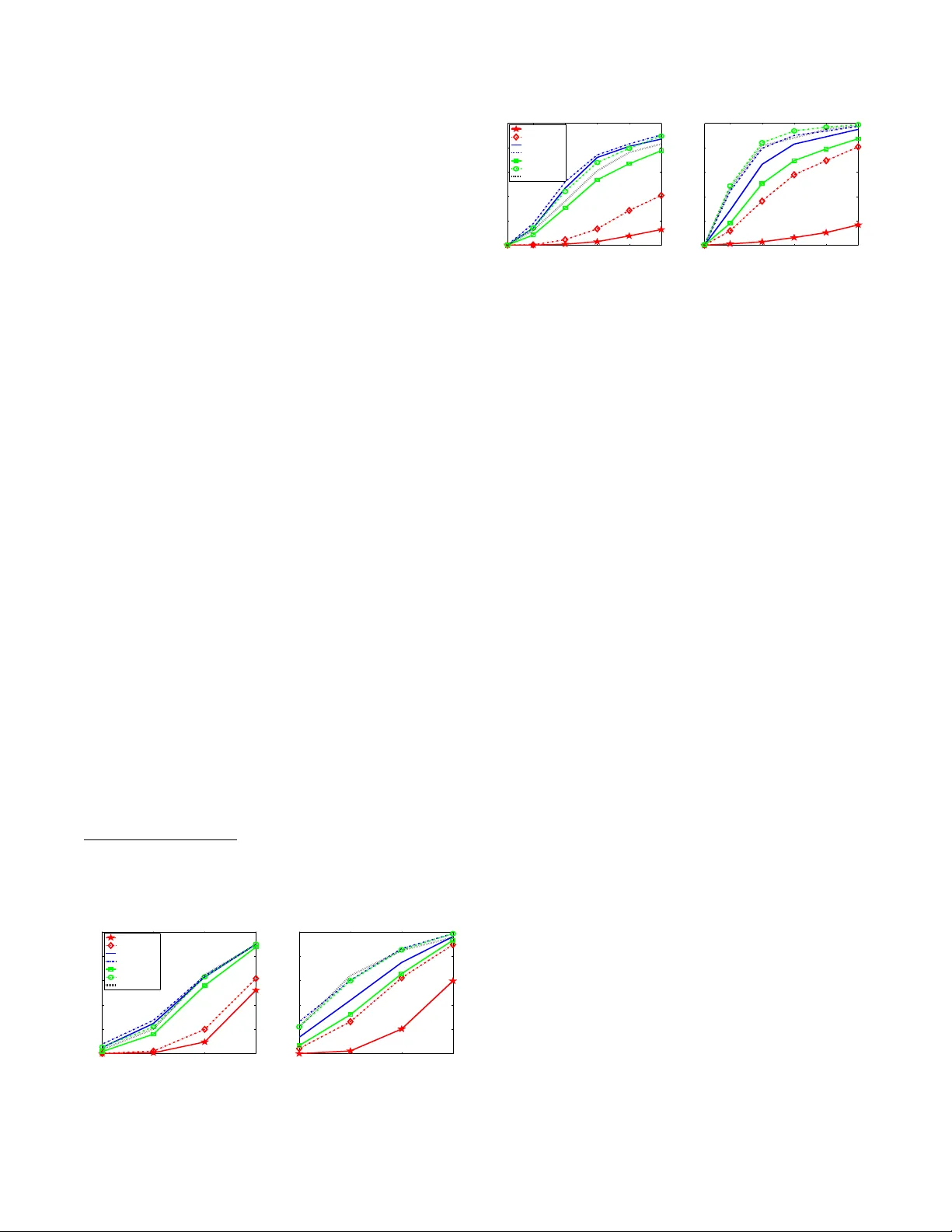
ITERA TIVE REWEIGHTED ALGORITHMS FOR SP ARSE SIGNAL RECO VER Y WITH TEMPORALL Y CORRELA TED SOURCE VECT ORS Zhilin Zhang and Bhaskar D. Rao Department of Electrical and Computer Engineering, Univ ersity of California at S an Diego, La Jolla, CA 92093-0407, USA { z4zhang,brao } @ucsd.edu ABSTRA CT Iterativ e rewe ighted algorithms, as a class of algorithms for sparse signal recov ery , hav e been found to hav e better performance than their non-reweighted counterparts. Ho we ver , for solving the prob- lem of multiple measurement vectors (MMVs), a ll the existing rewe ighted algorithms do not acco unt for temporal correlation among sou rce vectors and t hus their performance deg rades sig- nificantly in the presence of correlation. In this work we propose an iterativ e reweighted sparse Bayesian learning (SBL) algorithm ex- ploiting the temporal correlation, and moti v ated by it, we propose a strategy to improv e existing reweig hted ℓ 2 algorithms for t he MMV problem, i.e. replac ing their row norms with Mahalanob is distance measure. Simulations show that the proposed re weighted SBL al- gorithm has superior performance, and the proposed impro vemen t strategy is ef fective for e xisting re weighted ℓ 2 algorithms. Index T erms — S parse Signal Recovery , Compressi ve S ensing, Iterativ e Rewe ighted ℓ 2 Algorithms, M ultiple Measurement V ectors, Sparse Bayesian Learning, Mahalano bis distance 1. INTRODUCTION The multiple measurement vector (MMV) model for sparse signal recov ery is gi ven by [1] Y = ΦX + V , (1) where Φ ∈ R N × M ( N ≪ M ) is the dictionary matrix whose any N columns are l inearly independent, Y ∈ R N × L is the measure- ment matrix consisting of L measurement vectors, X ∈ R M × L is the source matrix wit h each row representing a possible source, and V is the white Gaussian noise matrix with each entry satisfy- ing V ij ∼ N (0 , λ ) . The key assumption under the MMV model is that the support (i.e. locations of nonzero entries) of ev ery column vector X · i ( ∀ i ) 1 is identical (referred as the common sparsity as- sumption in the literature [1]). The MMV problem is often encoun- tered i n practical applications, such as neuroelectromagnetic source localization and direction-of-arri val estimation. Most algorithms for the MMV problem can be roughly di vided into greedy methods, methods based on mixed norm optimization, iterativ e re weighted methods, and Bayesian methods. Iterativ e re weighted methods hav e recei ved attention because of their improv ed performanc e co mpared to their non-re weighted coun- terparts [2, 3]. In [3], an iterativ e re weighted ℓ 1 minimization frame- work is employed. The framew ork can be directly u sed for the MMV The work wa s supported by NSF Grant CCF-0830612. 1 The i -th column of X is denoted by X · i . The i -th row of X is denoted by X i · (also cal led the i -th source). problem and many MMV alg orithms based on mixed norm optimiza- tion c an b e imp rov ed via the framew ork. On the o ther h and, iterati ve rewe ighted ℓ 2 algorithms were also prop osed [2, 4]. T he re weighted ℓ 2 minimization frame work for the MMV problem (in noisy case) computes the solution at the ( k + 1) -th iteration as follo ws 2 : X ( k +1) = arg min x k Y − ΦX k 2 F + λ X i w ( k ) i ( k X i · k q ) 2 (2) = W ( k ) Φ T  λ I + ΦW ( k ) Φ T  − 1 Y (3) where typically q = 2 , W ( k ) is a diagonal weighting matrix at the k - th iteration with i -th diagonal element being 1 /w ( k ) i , and w ( k ) i depends on t he previous esti mate of X . Recently , Wipf et al [2] unified most ex isting iterati ve reweighted algorithms as belonging to the family of separ able reweigh ted algorithms, whose weighting w i of a gi v en row X i · at each iteration is only a function of that indi- vidual row from the pre vious iteration. Further , they proposed non- separa ble reweighted algorithms via variational approache s, which outperform many e xisting separable re weighted algorithms. In our previou s work [5, 6] we sho wed that temporal correla- tion in sources X i · seriously deteriorates recov ery performance of existing algorithms and propo sed a block sparse Bayesian learning (bSBL) framew ork, i n which we incorp orated temporal correlation and deriv ed effe ctiv e algorithms. These algorithms operate i n the hyperparameter space, not in the source space as most sparse si g- nal recov ery algorithms do. T herefore, it is not clear what t he con- nection of the bSBL framew ork is to other sparse signal recove ry frame works, such as the reweighted ℓ 2 in (2). In this work, based on the cost function in the bSBL framew ork, we deri ve an itera- tiv e re weighted ℓ 2 SBL algorithm with superior performance, which directly operates in the source space. Furthermore, motiv ated by the intuition gained from the algorithm and analytical insights, we propose a strategy to modify existing re weighted ℓ 2 algorithms to incorporate temporal correlation of sources, and use two typical al- gorithms as illustrations. The strategy is sh o wn to be effecti ve . 2. THE BLOCK SP ARSE BA YESIAN LEARNING FRAMEWORK The block sparse Bayesian learning (bSBL) framewo rk [5, 6] trans- forms the MMV problem to a single measurement vector problem. This mak es the modeling of temporal correlation much easier . First, we assume the ro ws of X are mutually independen t, and the density of each ro w X i · is multi v ariate Gaussian, giv en by p ( X i · ; γ i , B i ) ∼ N ( 0 , γ i B i ) , i = 1 , · · · , M 2 For con ve nience , we omit the superscript, k , on the right hand side of learni ng rules in the follo wing. where γ i is a nonne gati ve hyperparameter controlling the row spar- sity of X as in the basic sparse Bayesian learning [7, 8 ]. When γ i = 0 , the associated i -th ro w of X becomes zero. B i is an un- kno wn positiv e definite correlation matrix. By letting y = vec( Y T ) ∈ R N L × 1 , D = Φ ⊗ I L 3 , x = vec ( X T ) ∈ R M L × 1 and v = vec( V T ) , where vec( A ) denotes the vectorization of the matrix A formed by st acking its columns i nto a single column vector , we can transform t he MMV model (1) to the block single v ector model as follows y = Dx + v . (4) T o elaborate on the block sparsity mod el (4), we rewrite it as y = [ Φ 1 ⊗ I L , · · · , Φ M ⊗ I L ][ x T 1 , · · · , x T M ] T + v = P M i =1 ( Φ i ⊗ I L ) x i + v , where Φ i is the i -th column of Φ , x i ∈ R L × 1 is the i -th block in x and i t is the transposed i -th ro w of X in the original MMV model (1), i. e. x i = X T i · . K nonzero rows in X means K nonzero blocks in x . T hus we refer to x as block-sparse. For the block model (4), the Gaussian lik elihood is p ( y | x ; λ ) ∼ N y | x ( Dx , λ I ) . The prior f or x is gi ven by p ( x ; γ i , B i , ∀ i ) ∼ N x ( 0 , Σ 0 ) , where Σ 0 is a block diagonal matri x with the i - th diagonal block γ i B i ( ∀ i ). Giv en the hyp erparameters Θ , { λ, γ i , B i , ∀ i } , the Maximum A Posterior (MAP) estimate of x can be directly obtained from the posterior of the model. T o estimate these hyperparam eters, we can use the T ype-II maximum li kelihoo d method [8], which marginalizes over x and then p erforms maximum likelihood estimation, leading to the cost function: L (Θ) , − 2 log Z p ( y | x ; λ ) p ( x ; γ i , B i , ∀ i ) d x = log | λ I + DΣ 0 D T | + y T ( λ I + DΣ 0 D T ) − 1 y , (5 ) where γ , [ γ 1 , · · · , γ M ] T . W e refer to the whole framework includ- ing the solution estimation of x and the hyperparameter estimation as the bSBL framew ork. Note that in contrast to the original SBL frame work, the bSBL framework models the temporal correlation structure of sources in the prior density via the matrix B i ( ∀ i ) . 3. ITERA TIVE REWEIGHTED SP ARS E BA YESIAN LEARNING ALGORITHMS Based on the cost function (5), we can deri ve efficient algorithms that exploit temporal correlation of sources [ 5, 6]. But these algorithms directly operate in the hyperparameter space (i. e. the γ -space). So, it is not clear what t heir connection is t o other sparse signal recov- ery algorithms that directly operate i n the source space (i.e. the X - space) by minimizing penalties on the sparsity of X . Particularly , it is interesting to see if we can transplant the ben efits gained from the bSBL framew ork to other sparse signal reco very frame works such as the it erativ e reweighted ℓ 2 minimization frame work (2), impro ving algorithms belonging to those framewo rks. Following the approach de velop ed by Wipf et al [2] for the single measurement vector prob- lem, in the following we use the duality theory [9] to obtain a pena lty in the source space, based on which we deriv e an i terativ e re weighted algorithm for the MMV problem. 3.1. Algorithms First, we find that assigning a d ifferen t co v ariance matrix B i to ea ch source X i · will result in overfitting in the learning of the hyperpa- 3 W e denote the L × L identity matrix by I L . When the dimension is e vident from t he context, for simplici ty we use I . ⊗ is the Kronecke r produc t. rameters. T o overcom e the ov erfitting, we simplify and consider us- ing one matrix B to model all the source cov ariance matrixes. Thus Σ 0 = Γ ⊗ B with Γ , diag([ γ 1 , · · · , γ M ]) . Simulations will show that this simplification leads to good results e ve n if dif ferent sources hav e dif ferent temporal correlations (see Section 5). In order to transform the cost fu nction (5) to th e source space, we use the identity: y T ( λ I + DΣ 0 D T ) − 1 y ≡ min x  1 λ k y − Dx k 2 2 + x T Σ − 1 0 x  , by which we can upper-bound the cost function (5 ) and obtain the bound L ( x , γ , B ) = log | λ I + D Σ 0 D T | + 1 λ k y − Dx k 2 2 + x T Σ − 1 0 x . By fi rst minimizing ove r γ and B and then minimizing ov er x , we can get the cost function in the source space: x = arg min x k y − Dx k 2 2 + λg TC ( x ) , (6) where the penalty g TC ( x ) is defined by g TC ( x ) , min γ  0 , B ≻ 0 x T Σ − 1 0 x + log | λ I + DΣ 0 D T | . (7) From the definition (7) we hav e g TC ( x ) ≤ x T Σ − 1 0 x + log | λ I + DΣ 0 D T | = x T Σ − 1 0 x + log | Σ 0 | + log | 1 λ D T D + Σ − 1 0 | + N L log λ ≤ x T Σ − 1 0 x + log | Σ 0 | + z T γ − 1 − f ∗ ( z ) + N L log λ where in the last inequality we hav e used the conjug ate relation log   1 λ D T D + Σ − 1 0   = min z  0 z T γ − 1 − f ∗ ( z ) . (8) Here we denote γ − 1 , [ γ − 1 1 , · · · , γ − 1 M ] T , z , [ z 1 , · · · , z M ] T , and f ∗ ( z ) is concav e conjugate of f ( γ − 1 ) , log | 1 λ D T D + Σ − 1 0 | . Fi- nally , reminding of Σ 0 = Γ ⊗ B , we have g TC ( x ) ≤ N L log λ − f ∗ ( z ) + M log | B | + M X i =1 h x T i B − 1 x i + z i γ i + L log γ i i . (9) Therefore, t o solve the problem (6 ) wi th (9), we can perform the coordinate descent method ov er x , B , z and γ , i.e, min x , B , z  0 ,γ  0 k y − Dx k 2 2 + λ h M X i =1  x T i B − 1 x i + z i γ i + L log γ i  + M log | B | − f ∗ ( z ) i . (10) Compared to the framewo rk ( 2), we can see 1 /γ i can be seen as t he weighting for the corresp onding x T i B − 1 x i . But instead of applyin g ℓ q norm on x i (i.e. the i -th row of X ) as done in existing iterative rewe ighted ℓ 2 algorithms, our algorithm computes x T i B − 1 x i , i.e. the quadratic Mahala nobis distance of x i and its mean vec tor 0 . By minimizing (10) ove r x , the updating rule for x is give n by x ( k +1) = Σ 0 D T ( λ I + DΣ 0 D T ) − 1 y . (11) According to the du al property [9], from the relation (8), the optimal z is directly giv en by z i = ∂ log | 1 λ D T D + Σ − 1 0 | ∂ ( γ − 1 i ) = Lγ i − γ 2 i T r h BD T i  λ I + DΣ 0 D T  − 1 D i i , ∀ i (12) where D i consists of columns of D from the (( i − 1) L + 1) -th to the ( iL ) -th. From (10) the optimal γ i for fi xed x , z , B i s giv en by γ i = 1 L [ x T i B − 1 x i + z i ] . Substituting Eq.(12) into it, we hav e γ ( k +1) i = x T i B − 1 x i L + γ i − γ 2 i L T r h BD T i  λ I + DΣ 0 D T  − 1 D i i , ∀ i (13) By minimizing (10) ov er B , the updating rule for B is giv en by B ( k +1) = B / k B k F , with B = M X i =1 x i x T i γ i . (14) The updating rules (11) (13) and ( 14) are our reweighted algo- rithm minimizing the pena lty based on quadratic Mahalanobis dis- tance of x i . Si nce for a give n i , the weighting 1 /γ i depends on the whole estimated source matrix in the previou s iterati on (via B and Σ 0 ), the algorithm is a nonsepar able reweighted algorithm. The complex ity of this algorithm is high because it learns the parameters in a higher dimensional space than the original problem space. For example, consider the bSBL f rame work, in which the dictionary matrix D is of t he size N L × M L , while in the original MMV model the dictionary matri x is of the si ze N × M . W e use an approximation to simplify the algorithm and dev elop an efficient v ariant. Using the approximation :  λ I N L + D Σ 0 D T  − 1 ≈  λ I N + Φ ΓΦ T  − 1 ⊗ B − 1 , (15) which takes the equal si gn when λ = 0 or B = I , the updating rule (11) can be transformed to X ( k +1) = WΦ T  λ I + ΦWΦ T  − 1 Y , (16) where W , d iag([1 /w 1 , · · · , 1 /w M ]) wi th w i , 1 /γ i . Using the same approximation, the last term in (13) becomes T r h BD T i  λ I N L + DΣ 0 D T  − 1 D i i ≈ T r h B ( Φ T i ⊗ I )  ( λ I N + Φ WΦ T ) − 1 ⊗ B − 1  ( Φ i ⊗ I ) i = L Φ T i ( λ I N + Φ WΦ T ) − 1 Φ i . Therefore, from the upda ting rule of γ i (13) we hav e w ( k +1) i = h 1 L X i · B − 1 X T i · + { ( W − 1 + 1 λ Φ T Φ ) − 1 } ii i − 1 . (17) Accordingly , the updating rule for B becomes B ( k +1) = B / k B k F , with B = M X i =1 w i X T i · X i · . (18) W e denote the updating rules (16) (17) and (18) by ReSB L-QM . W ith t he aid of singular v alue deco mposition, the computational complex ity of the algorithm is O ( N 2 M ) (The effect of L can be remov ed by using the strategy in [7]). 3.2. Estimate the Regularization Parameter λ T o estimate the regularization parameter λ , man y method s ha ve been proposed, such as the modified L-curve method [1]. Here, straight- forwardly following the Expectation-Maximization method in [5] and using the approximation (15), we deriv e a learning rule for λ , gi ven by : λ ( k +1) = 1 N L k Y − ΦX k 2 F + λ N T r  G ( λ I + G ) − 1  . where G , ΦWΦ T . 3.3. Th eoretical Analysis in the Noiseless Case For the noiseless inv erse problem Y = ΦX , denote the generating sources by X gen , which is the sparsest solution among all the pos- sible solutions. Assume X gen is full column-rank. Den ote t he true source number (i.e. the tr ue number of nonzero rows in X gen ) by K 0 . Now we hav e the follo wing result on the global minimum of the cost function (5): Theorem 1 In the noiseless case , assuming K 0 < ( N + L ) / 2 , for the cost function (5) the unique global minimum b γ = [ b γ 1 , · · · , b γ M ] pr oduces a sour ce esti mate b X that equals t o X gen irr espective of the estimated b B i , ∀ i , wher e b X is obtained from vec ( b X T ) = b x and b x is computed using Eq.(11). The proof is giv en i n [6]. The theorem implies that ev en i f the estimated b B i is dif ferent from the true B i , the estimated sources are the t rue sources at the global minimum of the cost function. There- fore the estimation error in b B i does not harm the recov ery of true sources. As a remind er , in deriving our algorithm, we assumed B i = B ( ∀ i ) to avoid o verfitting. The theorem ensures that this strategy doe s not harm the global minimum property . In our work [6] we hav e sho wn that B plays the role of whitening sources in the SB L procedure, which can be seen in our algorithm as well. T his give s us a moti v ation t o i mprov e some state-of-the-art rewe ighted ℓ 2 algorithms by whitening the estimated sources in their weighting rules and penalties, detailed in the next section . 4. MODIFY EXISTING REWE IGHTED ℓ 2 METHODS Moti v ated by the abov e results and our analysis in [6], we can modify many re weighted ℓ 2 algorithms via replacing the ℓ 2 norm of X i · by some suitable function of its Mahalanobis distance. Note that similar modifications can be applied on re weighted ℓ 1 algorithms. The reg ularized M-FOCUSS [1] i s a typical reweighted ℓ 2 al- gorithm, which solves a reweigh ted ℓ 2 minimization with weights w ( k ) i = ( k X ( k ) i · k 2 2 ) p/ 2 − 1 in each iteration. It is gi ven by X ( k +1) = W ( k ) Φ T  λ I + ΦW ( k ) Φ T  − 1 Y (19) W ( k ) = diag { [1 /w ( k ) 1 , · · · , 1 /w ( k ) M ] } w ( k ) i =  k X ( k ) i · k 2 2  p/ 2 − 1 , p ∈ [0 , 2] , ∀ i (20) W e can mod ify the algo rithm by chan ging (20) to the follo wing one: w ( k ) i =  X ( k ) i · ( B ( k ) ) − 1 ( X ( k ) i · ) T  p/ 2 − 1 , p ∈ [0 , 2] , ∀ i (21) The matrix B can be calculated using t he learning rule (18). W e denote the modified algorithm by tMFOCUSS . In [4] Chartrand and Y i n proposed an it erativ e reweighted ℓ 2 algorithm based o n the classic FOCUSS algorithm. Its MMV exten- sion (denoted by Iter-L2 ) changed (20) to: w ( k ) i =  k X ( k ) i · k 2 2 + ǫ  p/ 2 − 1 , p ∈ [0 , 2] , ∀ i (22) Their algorithm adopts the strategy: initially use a relativ ely large ǫ , then repeating t he process of decreasing ǫ after con ver gence and re- peating the iteration (19), dramatically improving the recovery abil- ity . Similarl y , we can modify the weighting (22) to the following rule incorporating the temporal correlation of sources: w ( k ) i =  X ( k ) i · ( B ( k ) ) − 1 ( X ( k ) i · ) T + ǫ  p/ 2 − 1 , p ∈ [0 , 2] , ∀ i (23) and adopts the same ǫ -decreasing st rategy . B i s also giv en by (18). W e denote the modified algorithm by tIter-L2 . The proposed tMFOCUS S and tIter-L2 hav e con ver gence prop- erties similar to M-FOCUSS and Iter-L2, respe ctiv ely . Due to space limit we omit t heoretical analysis, and instead, provide some repre- sentati ve simulation results in the ne xt section. 5. EXPE RIMENTS In our e xperiments, a dictionary matrix Φ ∈ R N × M was created with columns uniformly drawing from t he surface of a unit hyp er- sphere. The source matr ix X gen ∈ R M × L was randomly generated with K nonzero rows of unit norms, whose row locations were ran- domly chosen. Amplitudes of the i -th non zero row were generated as an AR( 1) process whose AR coefficient was denoted by β i 4 . Thus β i indicates t he temporal correlation of the i -th source. The mea- surement matrix was constructed by Y = ΦX gen + V , where V was a zero-mean homosced astic Gau ssian noise matrix with variance adjusted to have a desired value of SNR . For each different experi- ment setting, we repeated 500 trials and av eraged results. The perfor - mance measurement was the F ailure R ate defined in [7], which indi- cated the percentage o f failed trials in the 5 00 trials. When noise w as present, since we could not exp ect any algorithm to reco ver X gen ex- actly , we classifi ed a trial as a failure trial if the K largest estimated ro w-norms did n ot a lign with the suppo rt of X gen . The com pared al- gorithms included our proposed ReSBL-QM, tMFOCUSS, tIter-L2, the reweighted ℓ 2 SBL in [2] (denoted by ReSBL-L2), M-FOCUSS [1], Iter-L2 p resented in Section 4, and Candes’ reweighted ℓ 1 algo- rithm [ 3] (exten ded to the MMV case as suggested by [2], denoted by Iter-L1). For tMFOCUSS, M-FOCUSS, and Iter-L2, we set p = 0 . 8 , which ga ve the best perfo rmance in our simulations. For Iter-L1, we used 5 iterations. In the first expe riment we fixed N = 25 , M = 100 , L = 3 and SNR = 25dB . The nu mber of nonzero source s K va ried from 10 to 16. Fig.1 (a) sho ws the results when each β i was uniformly chosen from [0 , 0 . 5) at random. F ig.1 (b) shows the results when each β i was uniformly cho sen from [0 . 5 , 1) at random . In the second experiment we fixed N = 25 , L = 4 , K = 12 , and SNR = 25dB , while M/ N varied from 1 to 25. β i ( ∀ i ) in Fig.2 (a) and (b) were generated as in Fig.1 (a) and (b), respecti vely . This experimen t aims to see algorithms’ performance in highly underde- termined inv erse problems, which met in some applications such as neuroelectromag netic source localization. From the two experiments we can see that: (a) in all cases, the proposed ReSBL-QM has sup erior performanc e to othe r algorithms, 4 Since in our experiment s the m easurement vector number is very small ( L = 3 or 4 ), gene rating sourc es as AR(1) with v ariou s AR coef ficien t v alues is suf ficie nt. 10 12 14 16 0 0.2 0.4 0.6 0.8 1 Number of Nonzero Sources K Failure Rate ReSBL−QM ReSBL−L2 tMFOCUSS MFOCUSS tIter−L2 Iter−L2 Iter−L1 (a) Low Co rrelati on Case 10 12 14 16 0 0.2 0.4 0.6 0.8 1 Number of Nonzero Sources K Failure Rate (b) High Correl ation Case Fig. 1 . Performance when the nonzero source number changes. 5 10 15 20 25 0 0.2 0.4 0.6 0.8 1 M/N Failure Rate ReSBL−QM ReSBL−L2 tMFOCUSS MFOCUSS tIter−L2 Iter−L2 Iter−L1 (a) Lo w Correlati on Case 5 10 15 20 25 0 0.2 0.4 0.6 0.8 1 M/N Failure Rate (b) High Correl ation Case Fig. 2 . Performance when M / N changes. capable to recov er more sources and solve more highly underdeter- mined in verse problems; (b) without considering temporal correla- tion of sources, existing algorithms’ performance significantly de- grades with increasing correlation; (c) after incorporating the tempo- ral structures of sources, the modified algorithms, i.e. tMFOCUSS and tIter-L2, have better performance than the original M-FOCUS S and Iter-L2, respectiv ely . Also, we noted that our proposed al go- rithms are more effecti ve when the norms of sources hav e no l arge differe nce (results are not sho wn here due to space limit). 6. CONCLUS IONS In this paper , we deriv ed an iterative re weighted sparse Bayesian al- gorithm exploiting the temporal str ucture of sources. It s simplified v ariant was also obtained, which has less computational load. Moti- v ated by our analysis we modified some stat e-of-the-art re weighted ℓ 2 algorithms achiev ing improved performance. This work not only provid es some effecti ve reweighted algorithms, but also provides a strategy to design effectiv e reweighted algorithms enriching current algorithms on this topic. 7. REFE RENCES [1] S. F . Cott er and B. D. Rao, “Sparse solutions to linear in verse problems wi th multiple measurement vectors, ” IEE E T ra ns. on Signal Pr ocessing , v ol. 53, no. 7, 2005. [2] D. Wipf and S. Nagarajan, “Iterative re weighted ℓ 1 and ℓ 2 meth- ods for finding sp arse solutions, ” IEEE J ournal of Selected T op- ics in Signal Pro cessing , vol. 4, no. 2, 2010. [3] E. J. Candes and et al, “Enhancing sparsity by reweighted ℓ 1 minimization, ” J F ourier Anal Appl , vol. 14 , 2008. [4] R. Chartrand and W . Y in, “Iterative ly re weighted algorithms for compressi ve sensing, ” in IC ASSP 2008 . [5] Z. Zhang and B. D. Rao , “Sparse signal recov ery in th e p resence of correlated multiple measurement vectors, ” in ICASSP 2010 . [6] ——, “ Sparse sign al reco very with temporally correlated source vectors using sparse Bayesian learning, ” IEEE Jo urnal of Se- lected T opics in Signal Pro cessing , submitted. [7] D. P . Wipf and B. D. Rao, “ An empirical Bayesian st rategy for solving the simultaneous sparse approximation problem, ” IEEE T rans. on Signal Pr ocessing , vo l. 55, no. 7, 2007. [8] M. E. Tip ping, “ Sparse Bayesian learning and the relev ance vec- tor machine, ” J. Ma ch. Learn. Res. , v ol. 1, pp. 211–244, 2001. [9] S. Boyd and L. V andenberg he, Con vex Optimization . Cam- bridge Univ ersity Press, 2004.