Generic Controllability of 3D Swimmers in a Perfect Fluid

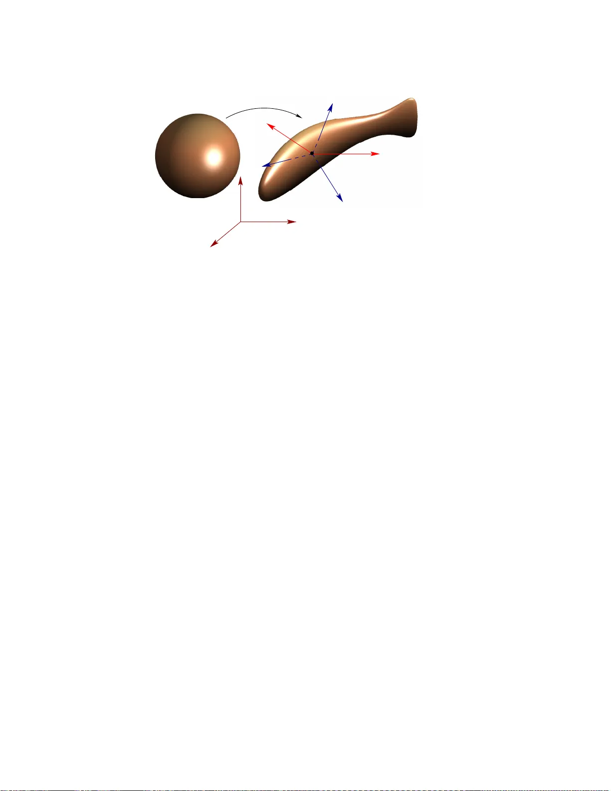
GENERIC CONTR OLLABILITY OF 3D SWIMMERS IN A PERFECT FLU ID THOMAS CHAMBRION ∗ AND ALEXANDRE MUNNIER ∗ † Abstract. W e address the problem o f con trolling a dynamical syste m gov e rning the motion of a 3D weigh ted shape c hanging body swimming in a perfect fluid. The rigid displacemen t of the swimmer results fr om the exchan ge of momen tum b e t we en prescrib ed shape c hanges and the flow, the tot al i mpulse of the fluid- swimmer s ystem b eing constan t for al l times. W e pro v e the f o llowing trac king results: (i) Sync h ronized swimmi ng : Ma ybe up to an arbitrarily small c han ge of its densit y , any swimmer can approximately f o llow an y given tra jectory while, in addition, undergoing approximately any give n shape changes. In this statemen t , the cont rol con sists in arbitraril y small superi mposed deform a tions; (ii) F reest yle swimming: Maybe up to an arbitrar ily small c hange of its density , any swimmer can approximately tracks any given tra jectory b y combining suitably at most five basic mov emen ts that can be generically ch osen (no macro shape change s are prescrib ed in this statemen t). Key words. Locomotion, Biomec hanics, Ideal fluid, Geomet ric control theo ry AMS sub ject cl a ssifications. 74F10, 70S05, 76B03, 93B27 1. In troductio n. 1.1. Con text. Researches on bio- inspired locomo t ion in fluid hav e no w a long history . F ocus - ing on the area of Mathematical Physics, the mo deling leads to a system of PDEs (governing the fluid flow) coupled with a system of ODEs (driving the rigid motion of the immersed bo dy). The first difficulty mathematicians c a me up against w as to prove the well-p osedness of such sy s t ems. This task was carr ied out in [16] (wher e the fluid is ass um ed to be viscous and gov erned by Navier Stokes equations), in [13] (for an inviscid fluid with po t ent ial flo w) and in [5] (for lo w Reynolds nu mbers swimmers , the flow b eing gov erned by the stationary Stokes e quations). After the w ell-po sedness of the fluid-swimmer dyna mics were es t ablished, the following s t ep was to investigate its controllability . On this topic, still few theoretical results a r e av ailable: In [2 ], the authors prove that a 3D three- sphere mechanism, swimming along a straight line in a viscous fluid is controllable. In [4], we prove that a generic 2D example of sha p e changing b ody swimming in a potential flow can track approximately a n y given tra jectory . Some authors ar e r ather in terested in describing the dyna mics of swimming in terms of Geo- metric Mechanics (within the genera l framework presented fo r instance in [12]). W e refer to [7] a nd the very recent pap er [8] for reference s in this a rea. In this article, we co nsider a 3D shap e c hanging b ody swimming in a p oten tial flow. Under some symmetry assumptions (the swimmer is alone in the fluid and the fluid-swimmer system fills the whole space) we prov e generic controllability res ults, g eneralizing a n d improving w ha t has been obtained for a par t icular 2D mo del in [4 ]. 1.2. Mo deling. Kinematics. W e assume that the swimmer is the only immersed b ody in the fluid and that the fluid-swimmer system fills the w ho le space, identified with R 3 . Two fra mes are required in the mo deling, the first one E := ( E 1 , E 2 , E 3 ) is fixed and Galilea n a nd the second one e := ( e 1 , e 2 , e 3 ) ∗ E-mail: thomas .chambrio n@iecn.u -nancy.fr and alexandre.m unnier@ie cn.u-nancy.fr † Both authors are wi t h Institut ´ Elie Cartan UMR 7502, Nancy-Universit ´ e, CNRS, INRIA, B.P . 239, F-54506 V andoeuvre-l` es-Nancy Cedex, F rance, and INRIA Nancy Grand Est, Pro jet CORID A. Authors b ot h supported by CPER MISN AOC. Fir st author s upproted by AN R GCM, ERC Boscain and INRIA color CUPIDSE, and second author b y ANR CISIFS, GA OS and M OSI COB. 1 is moving with its origin ly ing at any time at the center o f ma ss of the swimming bo dy . A t any moment, there exist a rotation matrix R ∈ SO(3) and a v ector r ∈ R 3 such that, if X := ( X 1 , X 2 , X 3 ) t and x := ( x 1 , x 2 , x 3 ) t are the co ordinates of a same v ector in resp ectiv ely E and e , then the equality X = Rx + r ho ld s. The matrix R is supp osed to g iv e also the orientation of the swimmer. The rig id dis pla cemen t of the s wim mer, on a time interv a l [0 , T ] ( T > 0), is thoroughly describ ed by the functions t : [0 , T ] 7→ R ( t ) ∈ SO(3) and t : [0 , T ] 7→ r ( t ) ∈ R 3 , which are the unknowns of our problem. Denoting their time deriv ativ es by ˙ R a nd ˙ r , w e can define the linear velocity v := ( v 1 , v 2 , v 3 ) t ∈ R 3 and angular velocity vector Ω := (Ω 1 , Ω 2 , Ω 3 ) t ∈ R 3 (bo t h in e ) by resp ectiv ely v := R t ˙ r and ˆ Ω := R t ˙ R , where for every vector u := ( u 1 , u 2 , u 3 ) t ∈ R 3 , ˆ u is the unique skew-symmetric matrix sa tis fying ˆ u x := u × x for ev ery x ∈ R 3 . V ectors of R 6 will sometimes b e deco mposed in the form f := ( f 1 , f 2 ) t ∈ R 3 × R 3 . F or every f := ( f 1 , f 2 ) ∈ R 6 and g := ( g 1 , g 2 ) ∈ R 6 , we can define f ⋆ g := ( f 1 × f 2 , f 1 × g 2 − g 1 × f 2 ) t ∈ R 6 . Shap e Changes. Unless otherwise indicated, from now on all of the qua n tit ies will be ex- pressed in the moving frame e . In our mo deling, the domains o ccupied by the swimmer are images of the closed unit ba ll ¯ B by C 1 diffeomorphisms, isotopic the the identit y , a n d tending to the ident it y at infinity , i.e. having the form Id + ϑ where ϑ b elongs to D 1 0 ( R 3 ) (definitions o f the function s paces are given in the app endix, Sectio n A). With these s e t tings, the shap e c hanges ov er a time interv al [0 , T ] can b e simply pr escribed by means of an absolutely co n tinuous function t ∈ [0 , T ] 7→ ϑ t ∈ D 1 0 ( R 3 ). Then, denoting Θ t = Id + ϑ t , the domain o ccupied by the swimmer at the time t ≥ 0 is the closed, b ounded, connected set ¯ B t := Θ t ( ¯ B ) (do not for get that we ar e working in the fr a me e ). W e still re q uire some notation: the unit ba ll’s bounda ry is Σ := ∂ B , Σ t := Θ t (Σ) stands fo r the b o dy-fluid interface, n t is the unit normal vector to Σ t directed toward the interior of B t and the fluid fills the exterior o pen set F t := R 3 \ ¯ B t . So-called self-p r op el le d cons t raints are nece s sary to ensure that the deformations r esult from the work of internal forces (they av oid for instance translations to b e consider ed as allow able shap e changes). L e t a function  ∈ C 0 ( ¯ B ) + be given. The density of the deformed b o dy at the insta n t t , denoted by  t ∈ C 0 ( ¯ B t ), is defined by:  t ( x ) :=  ( Θ − 1 t ( x )) /J t ( Θ − 1 t ( x )) , ( x ∈ ¯ B t , t ≥ 0 ) , (1.1) where J t := | det ∇ Θ t | = det ∇ Θ t (w e c an dro p the absolute v alue s her e b ecause Θ t ( x ) → x a s k x k R 3 → + ∞ and det ∇ Θ t ( x ) 6 = 0 fo r all x ∈ R 3 and t ≥ 0). The s elf-propelled co nstrain ts read: Z B t  t ( x ) x d x = 0 and Z B t  t ( x ) ∂ t Θ t ( Θ − 1 t ( x )) × x d x = 0 ( t ≥ 0) . (1.2a) The for mer iden tity means that, as alr eady mentioned b efore, the center of mas s of the swimmer lies at any time a t the or igin of the mo v ing frame. The latter rela t ion tells us that the angular momentum (in e ) ha s to remain constan t as the swimmer undergo es shap e changes. Equiv alent formulations can b e obtained up to a change of v aria bles : Z B  ( x ) Θ t ( x ) d x = 0 and Z B  ( x ) ∂ t Θ t ( x ) × Θ t ( x ) d x = 0 ( t ≥ 0 ) . (1.2b) The Flo w. The fluid is assumed to be in v iscid and incompress ible. W e denote by  f > 0 its consta n t density . The flo w is g overned b y Euler equatio ns. Accor ding to Helmholtz’s third 2 Ω e 2 e 3 e 1 Θ t B F t B t r E 3 E 2 E 1 0 v Fig. 1 . 1 . Kinematics of the mo del: The Galile an fr ame E := ( E j ) 1 ≤ j ≤ 3 and the moving fr ame e := ( e j ) 1 ≤ j ≤ 3 with e j = R E j ( R ∈ SO(3) ). Quantities ar e usual ly expr esse d in the moving fr ame. The domain of the b o dy is ¯ B t at the time t and B t is the image of the unit b al l B by a diffe omorphism Θ t . The op en set F t := R 3 \ ¯ B t is the domain of the fluid. The c enter of mass of t h e b o dy is denote d r (in E ), v : = R t ˙ r is its tr anslational velo city (in e ) and Ω its angular velo ci t y. theorem, if the flow is irrotatio na l at the initial time, it remains irr otational for all times. In this case, the Eulerian v e lo city is equal at a n y time to the gradient of a potential function. According to Kirchhoff ’s law, the p oten tial can b e deco mposed into a linear co m bination o f elementary p oten tials, each one connected to a degree of free do m of the s ystem (they consist here in the 6 degrees o f free dom of the rigid motion o f the b ody plus those connecting to the deformatio ns ) . These ideas have be e n thoroughly descr ibed in a series of pap ers [7, 13, 1 4, 4], to which we refer for further e xplanations. The elementary p oten tials ψ i t , ( i = 1 , . . . , 6 ) corr esponding to the rigid motion o f the swimmer are har monic in F t , tend to zer o as infinit y and satisfy the Neumann bounda ry co ndit ions ∂ n ψ i t = ( e i × x ) · n t ( i = 1 , 2 , 3) and ∂ n ψ i t = e i − 3 · n t ( i = 4 , 5 , 6) on Σ t . They are well defined in the weight ed Sob olev space W 1 ( F t ) (defined in the appendix, Sec tio n A ; see also [3 ] fo r details). The overall po ten tial connec t ing to the r igid displacement is ψ t := P 3 i =1 Ω i ψ i t + P 5 i =4 v i − 3 ψ i t ( t ≥ 0). On the other hand, the elemen ta ry potential ϕ t asso ciated to the shap e c ha nges, harmonic a s well in F t , satisfies the b oundary c o ndit ion ∂ n ϕ t = w t · n t on Σ t ( i = 1 , . . . , n ), wher e w t ( x ) := ∂ t Θ t ( Θ − 1 t ( x )) ( x ∈ R 3 ). Like the functions ψ i t ( i = 1 , 2 , 3), ϕ t belo ngs to W 1 ( F t ) for all t > 0. Dynamics. The modeling of moving rigid (or s ha pe changing) bo dies in an ideal fluid cla ssi- cally in volves the notion of mass matrices. The mass of the b ody is m := R B  d x and its inertia tensor at the time t ≥ 0 is defined by: I ( t ) := Z B t  t  k x k 2 R 3 Id − x ⊗ x  d x = Z B   k Θ t ( x ) k 2 R 3 Id − Θ t ( x ) ⊗ Θ t ( x )  d x. (1.3) W e in tro duce M r b ( t ) := diag ( I ( t ) , m Id ) (a 6 × 6 s ymmetric blo c diag onal matrix), M r f ( t ) (a 6 × 6 symmetric matrix as well) whose entries read:  f Z F t ∇ ψ i t · ∇ ψ j t d x, (1 ≤ i , j ≤ 6) , (1.4) 3 and we deno t e M r ( t ) := M r b ( t ) + M r f ( t ). W e also need the 6 × 1 column vector N ( t ), homogeneous to a moment um, whose element s read:  f Z F t ∇ ψ i t · ∇ ϕ t d x, (1 ≤ i ≤ 6) . (1.5) If we neglect the buoy a ncy force, it has b een proved in a s eries of pap ers (we refer for instance to the already men tioned articles [7 , 14] or [4]) that the swimming motion is gov er ned by the equatio n:  Ω v  = − M r ( t ) − 1 N ( t ) , ( t ≥ 0 ) . (1.6a) A t this p oin t, we ca n identified  t (or mor e simply  since they are linked through re lation (1.1)) as a pa rameter and the control as being the function t ∈ [0 , T ] 7→ ϑ t ∈ D 1 0 ( R 3 ). Notice that the depe nda nce of the dynamics in the control is strongly nonlinear. Indeed ϑ t describ es the shap e of the b ody and hence also the domain o f the fluid in which are set the PDEs of the potential functions inv olved in the expre s sions of the mass matr ic es M r ( t ) and N ( t ). T o determine the rigid mo tion, Eq ua tion (1.6 a) has to b e supplemented with the ODE: d dt  R r  =  R ˆ Ω R v  , ( t > 0 ) , (1.6b) together with Ca uc hy data for R (0) and r (0). Remark that the dynamics does not depend on  and  f independently but only on the relative density / f . So we can a ssume, without loss of generality , that  f = 1 in the sequel. 1.3. Main results . The first result ensures the well p osedness of System (1.6) and the conti- nu it y of the input-output mapping: Proposition 1.1. F or any T > 0 , any  ∈ C 0 ( ¯ B ) + , any absolutely c ontinu o u s function t ∈ [0 , T ] 7→ ϑ t ∈ D 1 0 ( R 3 ) (r esp e ctively of class C p , p = 1 , . . . , + ∞ or analytic) and any inital data ( R (0) , r (0)) ∈ SO(3) × R 3 , System (1.6) admits a u niq ue solution t ∈ [0 , T ] 7→ ( R ( t ) , r ( t )) ∈ SO(3) × R 3 (in the sense of Car ath´ eo dory) absolutely c ont i n uous on [0 , T ] (r esp e ctively of class C p or analytic). L et t ∈ [0 , T ] 7→ ϑ j t ∈ D 1 0 ( R 3 ) (for j = 1 , . . . , + ∞ ) b e a se quenc e of c ontr ols in AC ([0 , T ] , D 1 0 ( R 3 )) (se e Se ction A for a definition of this sp ac e) which c onver ges in t h is s p ac e to a fun c tion t ∈ [0 , T ] 7→ ¯ ϑ t ∈ D 1 0 ( R 3 ) . L et a p air ( R 0 , r 0 ) ∈ SO(3) × R 3 b e given and denote t ∈ [0 , T ] 7→ ( ¯ R ( t ) , ¯ r ( t )) ∈ SO(3) × R 3 the solution in AC ([0 , T ] , SO(3) × R 3 ) to System (1.6) with c ontro l ¯ ϑ and Cauchy data ( R 0 , r 0 ) . Then, t h e unique solution ( R j , r j ) to System (1.6) with c ont r ol ϑ j and Cauchy data ( R 0 , r 0 ) c onver ges in AC ([0 , T ] , SO(3) × R 3 ) to ( ¯ R, ¯ r ) as j → + ∞ . W e denote by M(3) the Ba nac h space of the 3 × 3 matrices endow ed wit any ma tr ix no rm. The main r e sult of this article a ddr esses the controllabilit y of System (1.6): Theorem 1.2. (Synchr onize d Swimming) Assume that the fol lowing data ar e given: (i) A function ¯  in C 0 ( ¯ B ) + (the t a rg et density of the swimmer); (ii) A C 1 function t ∈ [0 , T ] 7→ ¯ ϑ t ∈ D 1 0 ( R 3 ) (the tar get shap e changes) such that the p air ( ¯ , ¯ ϑ ) satisfies the self-pr op el le d c onstra int s (1.2) ; (iii) A C 1 function t ∈ [0 , T ] 7→ ( ¯ R ( t ) , ¯ r ( t )) ∈ SO(3) × R 3 (the tar get tr aje ctory to b e fol lowe d). Then, for any ε > 0 , ther e exists a function  ∈ C 0 ( ¯ B ) + (the actual density of the swimmer) and a function t ∈ [0 , T ] 7→ ϑ t ∈ D 1 0 ( R 3 ) (the actual shap e changes that c an b e chosen of class C p for any 4 p = 1 , . . . , + ∞ or even analytic) such t h at the p air ( , ϑ ) satisfies (1.2) , k ¯  −  k C 0 ( ¯ B ) < ε , ϑ 0 = ¯ ϑ 0 , ϑ T = ¯ ϑ T and sup t ∈ [0 ,T ]  k ¯ ϑ t − ϑ t k C 1 0 ( R 3 ) 3 + k ¯ R ( t ) − R ( t ) k M(3) + k ¯ r ( t ) − r ( t ) k R 3  < ε wher e the function t ∈ [0 , T ] 7→ ( R ( t ) , r ( t )) ∈ SO(3) × R 3 is the unique solution to system (1.6) with initial data ( R (0) , r (0)) = ( ¯ R (0) , ¯ r (0)) and c ont ro l ϑ . This theorem tells us that, maybe up to an arbitra rily small change o f its density , any weighted 3D b ody undergoing approximately any prescr ibed shap e changes can approximately track by swim- ming any given tra jector y . It may s e em surprising that the shap e changes, which are supp osed to be the co ntrol of our pro blem, can also be pr escribed. Actually , be aw ar e that they ar e only ap- pr oximately prescrib ed. W e ar e go ing to show prec is ely that arbitrarily small sup erimposed shap e changes suffice for con trolling the swimming mo t ion. This result improves what has b een done in the ar t icle [4] for a particula r 2D mo del. When no ma c ro s hape changes are presc r ibed we have: Theorem 1.3. (F r e estyle Swimming) Assume that the fol lowing data ar e given: (i) A p air ( ¯ , ¯ ϑ ) ∈ C 0 ( ¯ B ) + × D 1 0 ( R 3 ) satisfying (1.2) (the tar get density and shap e at r est) (ii) A C 1 function t ∈ [0 , T ] 7→ ( ¯ R ( t ) , ¯ r ( t )) ∈ SO(3) × R 3 (the tar get t r aje ctory). Then, for any ε > 0 t h er e exists a p air ( , ϑ ) ∈ C 0 ( ¯ B ) + × D 1 0 ( R 3 ) (the actual density and shap e at r est) such that (i) R B  Θ d x = 0 (wher e Θ := Id + ϑ ) (ii) k ¯  −  k C 0 ( ¯ B ) + k ¯ ϑ − ϑ k D 1 0 ( R 3 ) < ε and (iii) for almost any 5 -uplet ( V 1 , . . . , V 5 ) ∈ ( C 1 0 ( R 3 ) 3 ) 5 satisfying R B  V i d x = 0 , R B  Θ × V i d x = 0 and R B  V i × V j d x = 0 ( i, j = 1 , . . . , 5 ), ther e exists a function t ∈ [0 , T ] 7→ s ( t ) ∈ R 5 (that c an b e chosen of class C p for any p = 1 , . . . , + ∞ or even analytic) such that, using ϑ t := ϑ + P 5 i =1 s i ( t ) V i ∈ D 1 0 ( R 3 ) as c ontr ol in t h e dynamics (1.6) , we get sup t ∈ [0 ,T ]  k ¯ R ( t ) − R ( t ) k M(3) + k ¯ r ( t ) − r ( t ) k R 3  < ε wher e the function t ∈ [0 , T ] 7→ ( R ( t ) , r ( t )) ∈ SO(3 ) × R 3 is the unique solution to ODEs (1.6) with initial data ( R (0) , r (0)) = ( ¯ R (0) , ¯ r (0)) . Different ly stated, w e claim in this Theore m that any weigh ted 3D bo dy (maybe up to an arbitrar ily small change of its density) is a b le to swim b y means of allowable deformations (i.e. satisfying the self-pr opelled constra in ts) obtained as a s uit able combination of pretty m uch an y given five basic movemen ts. The pro ofs r ely on the following main ideas: Firs t , we shall identify a set of parameter s necessary to thoro ughly characterize a s wimm er and its w ay o f swimming (these parameters are its de ns it y , its shap e and a finite num b er of basic mov ements, sa tisfying the self-prop elled constraints (1.2)). An y s et o f such parameters will b e termed a swimmer c onfigu r ation (denoted SC in short). Then, the set o f all of the SC will be shown to b e an (infinite dimensional) ana ly t ic connected embedded submanifold o f a Ba nac h spac e . The second step of the reasoning will consist in proving that the swimmer’s abilit y to tra c k any given tra jectory (while under going any given shap e changes) is related to the v anishing of some analytic functions dep ending on the SC. These functions ar e connected to the determina n t of some vector fields and their Lie brackets (we will use here some classica l result of Geometric Con trol Theory). Even tually , b y direct calculation, we will prov e that a t least o ne swimmer (corr esponding to one particular SC) has this ability . An elementary prop ert y of analytic functions will even tually allow us to conclude that almo st any SC (or equiv ale ntly any s wim mer) ha s this prop ert y . Remark 1.4. The authors c onje ct u r e that in b oth The or em 1.2 and The or em 1.3, the actual density  c an b e chosen e qual to the t a rg et density ¯  . At this p oint howeve r and although it is very unlikely, it c an not b e exclude d that al l of t h e swimmers with a p articular density might b e unable to swim. This issue also app e ar e d in [4]. 5 1.4. Outline of the pap er. The next Section is dedicated to the notion of swimmer co n- figuration (definition and pro perties). In Sectio n 3 we show that the mass matrices are analytic functions in the SC (seen as a v ariable) and in Section 4 w e will restate the control proble m in order to fit with the gene r al framework of Geometric Co n trol Theo ry . A par t icular ca s e of sw immer will be shown to b e controllable. In Section 5 the pro of of the main results will b e p e r formed. Sectio n 6 contains some words of conclusion. Man y tec hnical results are gathered in the appendix to av oid ov erlo ading the rest of the pap er. 2. Swimmer Configuration. A swimmer c onfi g ur ation is a set of pa r ameters c hara cterizing swimmers whos e deformations consist in a combination of a finite num b er o f basic movemen ts. Definition 2 .1. F or any p ositive inte ger n , we denote C ( n ) the subset of C 0 ( ¯ B ) + × D 1 0 ( R 3 ) × ( C 1 0 ( R 3 ) 3 ) n c onsisting of al l of t h e triplets c := ( , ϑ, V ) such that, denoting Θ := Id + ϑ and V := ( V 1 , . . . , V n ) , the fol low ing c onditions hold (i) the set { V i | ¯ B · e k , 1 ≤ i ≤ n, k = 1 , 2 , 3 } is a fr e e family in C 1 0 ( ¯ B ) ( ii) every p air ( V , V ′ ) of elements of { Θ , V 1 , . . . , V n } satisfies R B  V d x = 0 and R B  V × V ′ d x = 0 . We c al l swimmer c onfigu ra t i on (SC in short) any element c of C ( n ) . By definition, D 1 0 ( R 3 ) is op en in C 1 0 ( R 3 ) 3 (see app endix, Section A). W e deduce that for a n y c ∈ C ( n ), the set { s := ( s 1 , . . . , s n ) t ∈ R n : ϑ + P n i =1 s i V i ∈ D 1 0 ( R 3 ) } is op en as well in R n and we denote S ( c ) its co nnected compo nen t containing s = 0. Definition 2.2. F or any p ositive inte ger n , we c al l extende d swimmer c onfigura t i on (ESC in short) any p air c := ( c, s ) such that c ∈ C ( n ) and s ∈ S ( c ) . We denote C X ( n ) the set of al l of these p airs. Restatement of the problem in terms of SC and ESC. Pick a SC in C ( n ) (for so m e int e ger n ). The characteris t ics of the corre sponding swimmer can be deduced from c as follows: If c is equal to ( , ϑ, V ) with V := ( V 1 , . . . , V n ), the shap e of the swimmer at rest is ¯ B := Θ ( ¯ B ) where Θ := Id + ϑ . When swimming, it can o ccupy the domains ¯ B c := Θ s ( ¯ B ) for all s ∈ S ( c ) ( c := ( c, s ) ∈ C ( n ) is hence an E SC) , where Θ s := Id + ϑ + P n i =1 s i V i . Still for any s ∈ S ( c ), its density is the function  s ∈ C 0 ( ¯ B c ) + defined by  s ( x ) :=  ( Θ − 1 s ( x )) /J s ( Θ − 1 s ( x )) with J s := det ∇ Θ s . Notice that within this constr uction, the shap e changes on a time interv al [0 , T ] ( T > 0) are merely given through an a bsolutely con tinuous function t : [0 , T ] 7→ s ( t ) ∈ S ( c ). If t ∈ [0 , T ] 7→ ˙ s ( t ) ∈ R n stands for its time deriv ative, the Lagr angian velocity at a p oin t x of ¯ B is P n i =1 ˙ s i ( t ) V i ( x ) while the Euleria n velocity at a p oint x ∈ ¯ B c is P n i =1 ˙ s i ( t ) w i s ( x ) where w i s ( x ) := V i ( Θ − 1 s ( x )). Due to assumption (ii) of Definition 2.1, the self-prop elled c o nstrain ts (1.2) are automatica lly sa tis fied. The harmo n ic elementary potential functions of the fluid c o rrespo nd ing to the rigid motions depe nd o nly on the ESC. Therefore , they will b e denoted in the seq uel ψ i c instead o f ψ i t . The same r emark ho lds for the iner t ia tenso r I ( t ) and the mass matrices M r ( t ), M r b ( t ) and M r f ( t ) whos e notation is tur ned into I ( c ), M r ( c ), M r b ( c ) and M r f ( c ) respe ct ively . The elemen tar y p oten tial connected to the shap e ch anges can be decompo s ed into P n i =1 ˙ s i ϕ i c . In this sum, each p oten tial function ϕ i c is har monic in F c := R 3 \ ¯ B c and sa t isfies on Σ c := ∂ B c the Neuma nn b oundary conditions ∂ n ϕ i c = w i s · n c , n c being the unit normal to Σ c directed to ward the int erior of B c . Int ro ducing the mass matrix N ( c ), whose elements are  f R B c ∇ ψ i c · ∇ ϕ j c d x (1 ≤ i ≤ 6 , 1 ≤ j ≤ n ) (recall that  f can b e chosen e q ual to 1), the dynamics (1 .6 a ) can now b e rewritten in the form:  Ω v  = − M r ( c ) − 1 N ( c ) ˙ s , ( t ≥ 0) . (2.1) 6 Let us fo cus on the prop erties of C ( n ) and C X ( n ). Theorem 2.3. F or any p ositive inte ger n , the set C ( n ) is an analytic c onne ct e d emb e dde d submanifold of C 0 ( ¯ B ) × C 1 0 ( R 3 ) 3 × ( C 1 0 ( R 3 ) 3 ) n of c o dimension N := 3( n + 2 )( n + 1) / 2 . The definition and the ma in pro perties of analytic functions in B a nac h spaces are summarized in the article [17]. Pr o of . F or any c := ( , ϑ, V ) ∈ C 0 ( ¯ B ) × C 1 0 ( R 3 ) 3 × ( C 1 0 ( R 3 ) 3 ) n , denote V 0 := Id + ϑ and V := ( V 1 , . . . , V n ). Then, define for k = 0 , 1 , . . . , n , the functions Λ k : C 0 ( ¯ B ) × C 1 0 ( R 3 ) 3 × ( C 1 0 ( R 3 ) 3 ) n → R 3( n +1 − k ) by Λ k ( c ) :=  R B  V k d x, R B  V k × V k +1 d x, . . . , R B  V k × V n d x  t . Every function Λ k is a nalytic and we draw the same conclusion for Λ := (Λ 0 , . . . , Λ n ) t : C 0 ( ¯ B ) × C 1 0 ( R 3 ) 3 × ( C 1 0 ( R 3 ) 3 ) n → R N ( N := 3( n + 2 ) ( n + 1) / 2 ) . In orde r to prove that ∂ c Λ( c ) (the differential of Λ at the p oin t c ) is onto for any c ∈ C ( n ), a ssume that there exist ( n + 2)( n + 1) / 2 vectors α j i ∈ R 3 (0 ≤ i ≤ j ≤ n ) such that: n X i =0 α i · h ∂ c Λ( c ) , c h i = 0 , ∀ c h ∈ C 0 ( ¯ B ) × C 1 0 ( R 3 ) 3 × ( C 1 0 ( R 3 )) 3 , (2.2) where α i := ( α i i , α i +1 i , . . . , α n i ) t ∈ R 3( n +1 − i ) ( j = 0 , . . . , n ) and c h := (  h , ϑ h , V h ) ∈ C 0 ( ¯ B ) × C 1 0 ( R 3 ) 3 × ( C 1 0 ( R 3 ) 3 ) n with V h 0 := Id + ϑ h and V h := ( V h 1 , . . . , V h n ). Reorg anizing the terms in (2.2), we obtain that: Z B  h h n X k =0 α k k · V k + X 0 ≤ i 0), X t =0 ( x ) = x is well defined (see [11, Theorem 1A, page 57]). Moreover, for every fixed t ∈ [0 , 1], the mapping x ∈ R 3 7→ X t ( x ) ∈ R 3 is C ∞ . Consider now the mappings t ∈ [0 , 1 ] 7→ ϑ t := X t ◦ ¯ Θ t − Id a nd Θ t := Id + ϑ t . If x ∈ R 3 \ ¯ Ω ′ , Θ t ( x ) = ¯ Θ t ( x ) for all t ∈ [0 , T ] and if x ∈ ¯ B then ϑ t ( x ) = ¯ ϑ t ( x ) + u ( t ) and Θ t ( x ) = ¯ Θ t ( x ) + u ( t ). Notice that ϑ t ∈ D 1 0 ( R 3 ) for all t ∈ [0 , T ] a nd R B  t ( x ) Θ t ( x )d x = 0 for all t ∈ [0 , T ]. Since C 1 0 ( R 3 ) 3 is a n infinite dimensional Bana ch spa c e , it is alwa ys p ossible to find b y induction W 1 , W 2 , . . . , W n in C 1 0 ( R 3 ) 3 such tha t (i) b oth fa milies { W 1 | ¯ B · e k , . . . , W n | ¯ B · e k , V † 1 | ¯ B · e k , . . . , V † n | ¯ B · e k , k = 1 , 2 , 3 } and { W 1 | ¯ B · e k , . . . , W n | ¯ B · e k , V ‡ 1 | ¯ B · e k , . . . , V ‡ n | ¯ B · e k , k = 1 , 2 , 3 } ar e free in C 1 0 ( R 3 ) a nd (ii) for any pair of elements V , V ′ ( b oth pick ed in the same family , R B  † V d x = 0 , R B  ‡ V d x = 0 , R B  † ¯ Θ j × V d x = 0 , R B  ‡ ¯ Θ j × V d x = 0 (for all j = 1 , . . . , k ), R B  † V × V ′ d x = 0 and R B  ‡ V × V ′ d x = 0 . Define the function t ∈ [0 , 1] 7→ V i t ∈ C 1 0 ( R 3 ) 3 by V i t := (1 − 2 t ) V † i + 2 t W i if 0 ≤ t ≤ 1 / 2 and V i t := (2 − 2 t ) W i + (2 t − 1) V ‡ if 1 / 2 < t ≤ 1 and denote V t := ( V 1 t , . . . , V n t ) ∈ ( C 1 0 ( R 3 ) 3 ) n . Even tua lly , a contin uous function linking c † to c ‡ is given by t ∈ [0 , 1] 7→ c t ∈ C ( n ) with c t := (  † , ϑ † , V 3 t/ 2 ) if 0 ≤ t ≤ 1 / 3, c t := (  3 t − 1 , ϑ 3 t − 1 , V 1 / 2 ) if 1 / 3 < t ≤ 2 / 3 and c t := (  ‡ , ϑ ‡ , V 3 t/ 2 − 1 / 2 ) if 2 / 3 < t ≤ 1. W e omit the pro o f o f the following cor ollary , similar to that of the theorem a b ov e: Corollar y 2. 4. F or any p ositive inte ger n , the set C X ( n ) is an analytic c onne ct e d emb e dde d submanifold of C 0 ( ¯ B ) × C 1 0 ( R 3 ) 3 × ( C 1 0 ( R 3 ) 3 ) n × R n of c o dimension N := 3( n + 2)( n + 1 ) / 2 . W e denote π the pro jection o f C ( n ) onto C 0 ( ¯ B ) × D 1 0 ( R 3 ) defined by π ( c ) = ( , ϑ ) for a ll c := ( , ϑ, V ) ∈ C ( n ). The pro of of the following corolla ry is a straig htf orward consequence of arguments alr eady used in the pr o of of Theo rem 2.3: Corollar y 2.5. F or any p ositive inte ger n and for any ( , ϑ ) ∈ π ( C ( n )) , the se ction π − 1 ( { ( , ϑ ) } ) is an emb e dde d c onne cte d analytic su bmanifold of {  }×{ ϑ }× ( C 1 0 ( R 3 ) 3 ) n (identifie d with ( C 1 0 ( R 3 ) 3 ) n ) of c o dimension 3 n ( n + 3) / 2 . 3. Sensitivity Analysis of the Mass M atrices. F or any p ositive in tegers k and p , we denote M( k , p ) the vector spac e of the matrices of siz e k × p (or s imply M( k ) when k = p ). Theorem 3.1. F or any p ositive inte ger n , the m appings c ∈ C X ( n ) 7→ M r ( c ) ∈ M(6) and c ∈ C X ( n ) 7→ N ( c ) ∈ M(6 , n ) ar e analytic. The metho d followed in this pr o of is inspire d from [6]. The result already appea red in [13], in a slightly different form though. Due to its crucia l imp or tance for our purp o se, we reca ll her e the 8 main idea s . Let us b eg in with a prelimina ry lemma o f whic h the statemen t requires intro ducing some material. Thus, we deno te F := R 3 \ ¯ B (r e call that B is the unit ball, Σ := ∂ B and n is the unit normal to Σ directed tow ar d the interior of B ). F or all ξ ∈ D 1 0 ( R 3 ), we set Ξ := Id + ξ , B ξ := Ξ ( B ), F ξ := Ξ ( F ), Σ ξ := Ξ (Σ) a nd n ξ stands for the unit norma l to Σ ξ directed tow ar d the in ter ior of B ξ . W e de no te q := ( ξ , W ), with W := ( W 1 , W 2 ) ⊂ ( C 1 0 ( R 3 ) 3 ) 2 , the elements of Q := D 1 0 ( R 3 ) × ( C 1 0 ( R 3 ) 3 ) 2 and w i ξ := W i ( Ξ − 1 ) ( i = 1 , 2). Finally , for ev ery q ∈ Q , we define: Φ ( q ) := Z F ξ ∇ ψ 1 q ( x ) · ∇ ψ 2 q ( x ) d x, (3.1) where, for every i = 1 , 2, the function ψ i q ∈ W 1 ( F ξ ) (rec all that the function spaces a re defined in Section A) is solution to the Laplace equation − ∆ ψ i q = 0 in F ξ with Neumann b oundar y data ∂ n ψ i q = w i ξ · n ξ on Σ ξ . The so lution ha s to b e under sto o d in the weak sense, na mely: Z F ξ ∇ ψ i q ( x ) · ∇ ϕ ( x ) d x = Z Σ ξ ( w i ξ · n ξ )( x ) ϕ ( x ) d σ, ∀ ϕ ∈ W 1 ( F ξ ) . (3.2) Lemma 3 .2. The mapping q ∈ Q 7→ Φ ( q ) ∈ R is analytic. Pr o of . W e pull back relation (3.2) onto the domain F using the diffeomorphism Ξ . W e get: Z F ∇ Ψ i q ( x ) A ξ ( x ) · ∇ ( ϕ ◦ Ξ )( x ) d x = Z Σ ( W i ( x ) · n ξ ( Ξ ( x )) ϕ ( Ξ ( x )) J σ ξ ( x ) d σ , ∀ ϕ ∈ W 1 ( F ξ ) , where Ψ i q := ψ i q ◦ Ξ , J ξ := det( ∇ Ξ ), A ξ := ( ∇ Ξ t ∇ Ξ ) − 1 J ξ and J σ ξ := k ( ∇ Ξ − 1 ) t n k R 3 J ξ (usually referred to a s the tangen tial J acobian). In (3 .2), if we spec ia lize the test function to have the form ϕ := φ ◦ Ξ − 1 with φ ∈ W 1 ( F ), we obtain R F Ψ i q ( x ) A ξ ( x ) · ∇ φ ( x ) d x = R Σ b i q ( x ) φ ( x ) d σ for all φ ∈ W 1 ( F ), where b i q := ( W i · n ξ ( Ξ )) J σ ξ ( i = 1 , 2). W e no w claim tha t the mapping ξ ∈ D 1 0 ( R 3 ) 7→ A ξ − Id ∈ E 0 0 (Ω , M(3)) is analytic. Indeed, the mappings ξ ∈ D 1 0 ( R 3 ) 7→ ∇ Ξ t ∇ Ξ − Id ∈ E 0 0 (Ω , M(3)), A ∈ E 0 0 (Ω , M(3)) 7→ (Id+ A ) − 1 − Id ∈ E 0 0 (Ω , M(3)) a nd ξ ∈ D 1 0 ( R 3 ) 7→ J ξ − 1 ∈ C 0 0 ( R 3 ) are analytic. Rea soning the s ame w ay , we ca n show that the mapping ξ ∈ D 1 0 ( R 3 ) 7→ J σ ξ ∈ C 0 (Σ) is analytic as w e ll (notice tha t for a ll ξ ∈ D 1 0 ( R 3 ), the function ( ∇ Ξ − 1 ) t n never v a nishes on Σ). It is more complicated to prove that ξ ∈ D 1 0 ( R 3 ) 7→ n ξ ◦ Ξ ∈ C 0 (Σ) 2 is analytic, so we refer to [13] for the details. This las t result entails the a nalyticity of q ∈ Q 7→ b i q ∈ C 0 (Σ). Then, denoting b y W 1 ( F ) ′ the dual space to W 1 ( F ), we cons ider the mapping Γ : ( q , u ) ∈ Q × W 1 ( F ) 7→ h A ξ , u, ·i − h b i q , ·i ∈ W 1 ( F ) ′ , where h A ξ , u, φ i := R F ∇ u ( x ) A ξ ( x ) · ∇ φ ( x ) d x and h b i q , φ i := R Σ b i q ( x ) φ ( x ) d σ ( φ ∈ W 1 ( F )). W e wish now to apply the implicit function theore m (analy tic version in Bana ch spaces, as stated in [17]) to the a nalytic function Γ . Observe, though, that w e a r e o nly interested in the regularity result and not in the existence a nd uniqueness. Indeed, we already kno w that for every q ∈ Q , there exists a unique function Ψ i q ∈ W 1 ( F ) such that Γ ( q , Ψ i q ) = 0 . The function Ψ i q is equal to ψ i q ◦ Ξ where ψ i q is the unique solution to the w ell posed v aria tional problem (3.2). The partial deriv ative ∂ u Γ ( q , Ψ i q ) is defined by: h ∂ u Γ ( q , Ψ i q ) , u, φ i = Z F ∇ u ( x ) A ξ ( x ) · ∇ φ ( x ) d x, ∀ φ ∈ W 1 ( F ) . (3.3) F or all ξ ∈ D 1 0 ( R 3 ), the matrix A ξ is uniformly elliptic in R 3 (there exists α ξ > 0 such that X t A ξ ( x ) X > α ξ k X k 2 R 3 for all X ∈ R 3 and all x ∈ R 3 ). W e deduce that the righ t hand side o f 9 (3.3) can b e chosen as the scalar product in W 1 ( F ) and hence that ∂ u Γ ( q , Ψ i q ) is a contin uous isomorphism from W 1 ( F ) onto its dual space according to the Riesz repr esentation theorem. The implicit function theorem a pplies and as serts that the mapping q ∈ Q 7→ Ψ i q ∈ W 1 ( F ) is analytic. T o co nclude the pro of, it remains o nly to obs e rve that the function Φ ( q ) introduced in (3.1 ) ca n be rewr itten, up on a change of v ar iables as Φ ( q ) = R F ∇ Ψ 1 q ( x ) A ξ ( x ) · ∇ Ψ 2 q ( x ) d x , whic h is indeed analytic as a comp ositio n of ana ly tic functions. W e can now give the pro o f of Theorem 3.1. Pr o of . Recall that the e le ment s of the matrix M r f ( c ) are defined in (1.4) and thos e o f N ( c ) in (1.5). F or any c := ( c, s ) ∈ C X ( n ), where c := ( , ϑ, V ), w e a pply the lemma with ξ := ϑ + P n i =1 s i V i and W 1 , W 2 ∈ { e i × Ξ , e i , i = 1 , 2 , 3 } to get that the mapping c ∈ C X ( n ) 7→ M r f ( c ) ∈ M(6) is analy tic. T o prove the analyticity of the elemen ts o f N ( c ), we apply the lemma again with ξ := ϑ + P n i =1 s i V i , W 1 ∈ { e i × Ξ , e i , i = 1 , 2 , 3 } and W 2 ∈ { V 1 , . . . , V n } . Even tually , the analyticity of the elemen ts of M r b ( c ) is s traightforward after rewriting the inertia tenso r I ( c ) defined in (1 .3) in the form (up on a change of v a r iables) I ( c ) = R B  [ k Ξ k 2 R 3 Id − Ξ ⊗ Ξ ] d x , still with Ξ := Id + ξ and ξ := ϑ + P n i =1 s i V i . 4. Con trol . 4.1. Con troll able SC. Let us fix c ∈ C ( n ) (for some p o sitive integer n ) and recall that S ( c ) is the connected op en subspa ce of R n such that ( c, s ) ∈ C X ( n ). Intro ducing ( f 1 , . . . , f n ) an ordered orthonor mal basis o f R n , w e can seek the function t ∈ [0 , T ] 7→ s ( t ) ∈ S ( c ) as the solution o f the ODE ˙ s ( t ) = P n i =1 λ i ( t ) f i where the functions λ i : t ∈ [0 , T ] 7→ λ i ( t ) ∈ R are the new controls, and rewrite onc e more the dynamics (2.1) a s:   Ω v ˙ s   = n X i =1 λ i ( t )  − M r ( c, s ) − 1 N ( c, s ) f i f i  , ( t ≥ 0 ) . (4.1) It is worth remark ing tha t in this form, s is no more the control but a v ariable which is mea nt to b e controlled and c ∈ C ( n ) is a par ameter of the dy namics. Considering (4.1), we are quite na turally led to in tro duce, for all c ∈ C X ( n ), the vector fields X i ( c ) := − M r ( c ) − 1 N ( c ) f i ∈ R 6 , Y i ( c ) := ( ˆ X 1 i ( c ) , X 2 i ( c ) , f i ) t ∈ T Id SO(3) × R 3 × R n (w e have us ed here the notation X i := ( X 1 i , X 2 i ) t ∈ R 3 × R 3 ) and Z i c ( R, s ) := R R Y i ( c ) ∈ T R SO(3) × R 3 × R n where R R := diag( R, R , Id) ∈ SO(6 + n ) is a blo c diagonal matrix. The dynamics (4.1) and the ODE (1.6 b) can b e ga thered into a unique differential sys tem: d dt   R r s   = n X i =1 λ i ( t ) Z i c ( R, s ) , ( t ≥ 0) . (4.2) F or ev e ry i = 1 , . . . , n , the function ( R, r , s ) ∈ SO(3) × R 3 × S ( c ) 7→ Z i c ( R, s ) ∈ T R SO(3) × R 3 × R n can be seen as an a nalytic vector field (constant in r ) o n the analytic connected manifold M ( c ) := SO(3) × R 3 × S ( c ). W e denote ζ a ny element ( R, r , s ) ∈ M ( c ) and we define Z ( c ) as the family of vector fields ( Z i c ) 1 ≤ i ≤ n on M ( c ). Lemma 4.1. L et c b e a S C fix e d in C ( n ) ( n a p ositive inte ger). If ther e exists ζ ∈ M ( c ) such that dim Lie ζ Z ( c ) = 6 + n , then the orbit of Z ( c ) thr ough any ζ ∈ M ( c ) is e qual to t he whole manifold M ( c ) . Pr o of . Rashevsky Cho w Theorem (see [1]) applies: If Lie ζ Z ( c ) = T ζ M ( c ) for all ζ ∈ M ( c ) (or mor e precisely , for all ( R, s ) ∈ SO(3) × S ( c ) since Z i c do es not depend on r ) then the orbit of 10 Z ( c ) thr ough any p oint of M ( c ) is equal to the whole manifold. L et us co mpute the Lie brack e t [ Z i c ( R, s ) , Z j c ( R, s )] fo r 1 ≤ i, j ≤ n and ( R, s ) ∈ SO(3 ) × S ( c ). W e get: [ Z i c ( R, s ) , Z j c ( R, s )] = R R    \ ( X 1 i × X 1 j )( c ) ( X 1 i × X 2 j − X 1 j × X 2 i )( c ) 0    + R R    \ ( ∂ s i X 1 j − ∂ s j X 1 i )( c ) ( ∂ s i X 2 j − ∂ s j X 2 i )( c ) 0    . (4.3) By induction, we can similarly prove that the Lie br ack ets of any or der a t a ny po int ζ ∈ M ( c ) hav e the same g eneral form, namely the matrix R R m ultiplied by an element of T (Id , 0 ,s ) M ( c ). W e deduce that the dimension of the Lie alge bra at any p oint o f M ( c ) dep ends only on s . According to the Orbit Theorem (see [1]), the dimensio n of the Lie algebra is constant a lo ng any orbit. But according to the par ticular form of the vector fields Z i c (whose las t n compo nents form a basis of R n ), the pro jection of any orbit on S ( c ) turns out to b e the whole set S ( c ) (or, in other words, for any s ∈ S ( c ) and for a ny or bit, there is a po int of the orbit for whic h the last comp onent is s ). Assume now that dim Lie ζ ∗ Z ( c ) = 6 + n at some particular po int ζ ∗ := ( R ∗ , r ∗ , s ∗ ) ∈ M ( c ). Then, according to the Orbit Theor em, for a ny s ∈ S ( c ), there ex ists at lea st one p o int ( R s , r s , s ) ∈ M ( c ) such that dim Lie ( R s , r s ,s ) Z ( c ) = 6 + n . But since the dimension of the Lie algebr a do es not dep end on the v ar iables R and r , w e conclude tha t dim Lie ζ Z ( c ) = 6 + n for all ζ ∈ M ( c ). Definition 4.2. We say that c , a SC in C ( n ) (for some int e ger n ) is c ontr ol lable if ther e exists ζ ∈ M ( c ) such that dim Lie ζ Z ( c ) = 6 + n . It is obvious that for a SC to be controllable, the integer n has to be larger or equal to 2. The following result is quite classical (a pro of ca n b e found in [4]): Proposition 4.3. L et c ∈ C ( n ) (for some inte ger n ) b e c ontr ol lable (with the u sual notation c := ( , ϑ, V ) , V := ( V 1 , . . . , V n ) and ϑ s := ϑ + P n i =1 s i V i for every s ∈ S ( c ) ). Then for any given c ontinuous function t ∈ [0 , T ] 7→ ( ¯ R ( t ) , ¯ r ( t ) , ¯ s ( t )) ∈ SO(3) × R 3 × S ( c ) and for any ε > 0 , ther e exist n C 1 functions λ i : [0 , T ] → R ( i = 1 , . . . , n ) such that: 1. sup t ∈ [0 ,T ]  k ¯ R ( t ) − R ( t ) k M(3) + k ¯ r ( t ) − r ( t ) k R 3 + k ϑ ¯ s ( t ) − ϑ s ( t ) k C 1 0 ( R 3 ) 3  < ε ; 2. R ( T ) = ¯ R ( T ) , r ( T ) = ¯ r ( T ) and s ( T ) = ¯ s ( T ) ; wher e t ∈ [0 , T ] 7→ ( R ( t ) , r ( t ) , s ( t )) ∈ M ( c ) is the unique solution to the O DE (4.2) with Cauchy data R (0 ) = ¯ R (0) ∈ SO(3) , r (0) = ¯ r (0) ∈ R 3 , s (0) = ¯ s (0) ∈ S ( c ) . Let us mention so me other quite elementary pr o p erties that will b e used later on: Proposition 4.4. 1. If c := ( , ϑ, V ) ∈ C ( n ) ( n ≥ 2) is a c ontr ol lable SC with V := ( V 1 , . . . , V n ) ∈ ( C 1 0 ( R 3 ) 3 ) n then any c + := ( , ϑ, V + ) ∈ C ( n + 1) su ch t hat V + := ( V 1 , . . . , V n , V n +1 ) ∈ ( C 1 0 ( R 3 ) 3 ) n +1 (for some V n +1 ∈ C m 0 ( R 3 ) 3 ) is a c ont r ol lable SC as wel l. 2. If c := ( , ϑ, V ) ∈ C ( n ) ( n ≥ 2) is a c ontr ol lable SC, then for any ϑ ∗ ∈ { ϑ + P n i =1 s i V i , s ∈ S ( c ) } the element c ∗ := ( , ϑ ∗ , V ) b elongs t o C ( n ) and is a c ontr ol lable SC as wel l. 3. If c := ( , ϑ, V ) ∈ C ( n ) ( n ≥ 2) is a c ontr ol lable SC, then al l of the c ont ro l lable SC c ∗ := ( , ϑ, V ∗ ) in C ( n ) ( V ∗ ∈ ( C 1 0 ( R 3 ) 3 ) n ) form an op en dense subset of the se ction π − 1 ( { ( , ϑ ) } ) (for t he induc e d top olo gy). 4. If ther e exists a SC in C ( n ) for some n ≥ 2 then, for any k ≥ n , al l of the c ontr ol lable SC in C ( k ) form an op en dense subset of C ( k ) (for the induc e d top olo gy). Pr o of . The t wo first assertio ns are o bvious so let us address dire ctly the third po int. Denote E k ( k p ositive integer) the set of all of the vectors fields o n M ( c ) obtained as Lie brackets of order low er or equal to k from elements of Z ( c ). Then, consider the determinants of all of the different families of 6 + n e lements of E k as a nalytic functions in the v aria ble V (the other v ar iables  , ϑ and 11 s = 0 b eing fixed). Since c is controllable, there exist at least one k and one family of 6 + n elemen ts in E k whose determinant is nonzero. Acco rding to Cor ollary 2.5 and bas ic prop erties of analytic functions (see [17]), the determinant may v a nish only in a closed subset with empt y int erior of the section π − 1 ( { ( , ϑ ) } ) (for the induced topo logy). The pr o of of the last point is simila r. 4.2. Building a controllable SC. In this subsectio n, we are in tere s ted in computing the Lie brack ets of fir st or der [ Z i c ( R, s ) , Z j c ( R, s )] a t ( R , s ) = (Id , 0 ), for a particular SC. General computations. Star ting from identit y (4.3) and focus ing on the seco nd term in the right ha nd side, we hav e, for all c ∈ C ( n ) ( n ≥ 2) , all s ∈ S ( c ) a nd all i, j = 1 , . . . , n : ∂ s i X j ( c ) − ∂ s j X i ( c ) = M r ( c ) − 1 h ( ∂ s j M r ( c ) X i ( c ) − ∂ s i M r ( c ) X j ( c )) + ( ∂ s j N ( c ) f i − ∂ s i N ( c ) f j ) i . (4 .4) F rom the deco mp o sition M r ( c ) := M r b ( c ) + M r f ( c ), we deduce that: ∂ s j M r ( c ) X i ( c ) − ∂ s i M r ( c ) X j ( c ) = ( ∂ s j M r b ( c ) X i ( c ) − ∂ s i M r b ( c ) X j ( c )) + ( ∂ s j M r f ( c ) X i ( c ) − ∂ s i M r f ( c ) X j ( c )) . (4 .5) W e ca n easily c ompute the firs t term in the right hand side whe n s = 0. Thus, for all i , j = 1 , . . . , n , we hav e: [ ∂ s j M r b ( c ) X i ( c ) − ∂ s i M r b ( c ) X j ( c )] s =0 = η j  Id 0 0 0  X i ( c ) | s =0 − η i  Id 0 0 0  X j ( c ) | s =0 , (4.6) where η i := 2 R B  ( x ) V i ( x ) · Θ ( x ) d x . Rigid she ll’s deformation. W e consider now shap e c ha nges that reduce to rigid dis pla ce- men ts on the swimmer’s b oundary Σ (but obviously not inside the b o dy for the self-pro p elled constraints not to b e violated). The idea of using such defor mations s temmed from the reading of the article [9]. How ever, rig id deformations of the shell can not be considered within the mo d- eling describ ed in Section 2 (because rigid deforma tions do not fit with the gener al form of the diffeomorphisms desc r ib ed in Sec tio n 2). Le t us explain how to deal with this difficult y . Let c := ( , ϑ, V ) ∈ C (6) b e given such that V := ( V 1 , . . . , V 6 ) with V i | Σ ( x ) := e i × ( x + ϑ ( x )) ( i = 1 , 2 , 3) a nd V i | Σ ( x ) := e i − 3 ( i = 4 , 5 , 6) (Pr op osition C.1 in the app endix gua rantees the existence of such vector fields sa tisfying furthermo re η i = 0 for a ll i = 1 , . . . , 6). T hus, the shap e changes we are considering r ead Θ s := Id + ϑ + P 6 i =1 s i V i ( s ∈ S ( c )). Let us define also Ξ s := R s (Id + ϑ ) + τ s where R s := exp( s 1 ˆ e 1 ) exp( s 2 ˆ e 2 ) exp( s 3 ˆ e 3 ) ∈ SO(3) and τ s := P 3 i =1 s i +3 e i ∈ R 3 . Thu s, Θ s is a diffeomor phism which can be achiev ed within our mo de ling while Ξ s is a tru e rigid deformation. In order to determine the expressions of the terms ∂ s i M r f ( c ) | s =0 ( i = 1 , . . . , 6) a rising in the computation o f the Lie brack ets, we ha ve to co mpare (using the notation of Lemma 3.2) ∂ s i Φ ( q 1 s ) | s =0 and ∂ s i Φ ( q 2 s ) | s =0 ( i = 1 , . . . , 6) where: • q 1 s := ( ξ 1 s , W 1 s ) with ξ 1 s := Ξ s − Id, W 1 s := ( W 1 , 1 s , W 1 , 2 s ) and W 1 , 1 s , W 1 , 2 s ∈ { e i × Ξ s , e i , i = 1 , 2 , 3 } (settings corresp onding to a true rigid deformatio n of the shell); • q 2 s := ( ξ 2 s , W 2 s ) with ξ 2 s := Θ s − Id = ϑ + P n i =1 s i V i , W 2 s := ( W 2 , 1 s , W 2 , 2 s ) and W 2 , 1 s , W 2 , 2 s ∈ { e i × Θ s , e i , i = 1 , 2 , 3 } (settings allow ed in o ur mo deling). 12 Remark that ∂ s i Θ s | s =0 = ∂ s i Ξ s | s =0 on Σ fo r all i = 1 , . . . , 6 , so the defor mations are tangent at s = 0. It entails that ∂ s i q 1 s | s =0 = ∂ s i q 2 s | s =0 . Since, in addition, q 1 s =0 = q 2 s =0 and ∂ s i Φ ( q k s ) | s =0 = h ∂ q Φ ( q k s ) , ∂ s i q k s i| s =0 for k = 1 , 2 a nd i = 1 , . . . , 6, we deduce that ∂ s i Φ ( q 1 s ) | s =0 = ∂ s i Φ ( q 2 s ) | s =0 for all i = 1 , . . . , 6. W e apply the diffeomorphism Ξ s := R s (Id + ϑ ) + τ s to ¯ B to obtain the domain of the deformed swimmer. W e denote B ⋄ := (Id + ϑ )( B ) (whic h can be see n as the shap e of the swimmer at rest, i.e. when s = 0), Σ ⋄ := ∂ B ⋄ , F ⋄ := R 3 \ ¯ B ⋄ and B s := Ξ s ( B ), F s := R 3 \ ¯ B s , Σ s := ∂ B s . W e seek the po tential ψ 1 c , defined a nd harmonic in F s in the for m ψ 1 c ( x ) = ˜ ψ 1 c ( R t s ( x − τ s )) wher e the function ˜ ψ 1 c defined on F ⋄ has to be determined. It is o bvious tha t ˜ ψ 1 c is harmonic in F ⋄ and we hav e only to determine the b oundar y c o nditions on Σ ⋄ . F or all y ∈ Σ ⋄ , we denote x := R s y + τ s ∈ Σ s . The relation n | Σ s ( R s y + τ s ) = R s n | Σ ⋄ ( y ) e nt ails that ∇ ˜ ψ 1 c ( y ) · n | Σ ⋄ ( y ) = ∇ ψ 1 c ( R s y + τ s ) · n | Σ s ( R s y + τ s ) = ∇ ψ 1 c ( x ) · n ( x ), and this quantit y ha s to b e equal to ( e 1 × x ) · n ( x ). W e deduce a fter some elementary algebra that ∂ n ˜ ψ 1 c ( y ) = ( R t s e 1 × y ) · n ( y ) + ( R t s e 1 × R t s τ s ) · n ( y ). Pro c eeding similarly and with obvious notatio n, we obtain more generally that: ∂ n ˜ ψ i c ( y ) = ( R t s e i × y ) · n ( y ) + ( R t s e i × R t s τ s ) · n ( y ) , ( i = 1 , 2 , 3) , and ∂ n ˜ ψ i c ( y ) = R t s e i − 3 · n ( y ) , ( i = 4 , 5 , 6) . Denoting M ⋄ f := M r f ( c ) | s =0 , we get the r elations: M r f ( c, s ) =  Id ˆ τ s 0 Id   R s 0 0 R s  M ⋄ f  R t s 0 0 R t s   Id 0 − ˆ τ s Id  , and then, differentiating with resp ect to s i : ∂ s i M r f ( c, s ) | s =0 =  ˆ e i 0 0 ˆ e i  M ⋄ f − M ⋄ f  ˆ e i 0 0 ˆ e i  , ( i = 1 , 2 , 3) , (4.7a) ∂ s i M r f ( c, s ) | s =0 =  0 ˆ e i − 3 0 0  M ⋄ f − M ⋄ f  0 0 ˆ e i − 3 0  , ( i = 4 , 5 , 6) . (4.7b) The rea soning is quite simila r for the ent ries of the matrix N ( c ). W e only hav e to b e care- ful that the vector fields W 2 , 2 s can ac tually not dep end on s (once more, this is due to our mo deling). The elements of the matrix ∂ s j N ( c ) | s =0 f i − ∂ s i N ( c ) | s =0 f j read (still with the nota- tion of Lemma 3.2) ∂ s j Φ ( q i s ) | s =0 − ∂ s i Φ ( q j s ) | s =0 ( i, j = 1 , . . . , 6) with this time q i s := ( ξ s , W i s ), ξ s := Ξ s − Id, W i s := ( W 1 s , W i, 2 ), W 1 s ∈ { e k × Ξ s , e k , k = 1 , 2 , 3 } and W i, 2 := e i × (Id + ϑ ) ( i = 1 , 2 , 3) o r W i, 2 = e i − 3 ( i = 4 , 5 , 6). The only difference with the elements o f M r f ( c ) being that W i, 2 do es not dep end on s for i = 1 , 2 , 3 , we wish to r euse the prec e ding calcula- tions. Inv ok ing the chain rule, we have to s ubtract to ∂ s j Φ ( q i s ) | s =0 − ∂ s i Φ ( q j s ) | s =0 the quan tity h ∂ W 2 Φ ( q i s ) , ∂ s j W i, 2 s i| s =0 − h ∂ W 2 Φ ( q j s ) , ∂ s i W j, 2 s i| s =0 which is quite easy to deter mine beca use Φ is linear in the v ar iable W 2 . Thus, this last expr ession is merely equa l to Φ ( q i,j ) (1 ≤ i, j ≤ 6) with q i,j := ( ϑ, W i,j ), W i,j := ( W 1 , W 2 i,j ), W 1 ∈ { e k × (Id + ϑ ) , e k , k = 1 , 2 , 3 } and W 2 i,j :=          ( e i × e j ) × (Id + ϑ ) if 1 ≤ i, j ≤ 3 , ( e i × e j ) if 4 ≤ i ≤ 6 , 1 ≤ j ≤ 3 , ( e i × e j ) if 1 ≤ i ≤ 3 , 4 ≤ j ≤ 6 , 0 if 4 ≤ i, j ≤ 6 . 13 W e even tually obtain that: ∂ s j N ( c ) | s =0 f i − ∂ s i N ( c ) | s =0 f j = ∂ s j M r f ( c ) | s =0 f i − ∂ s i M r f ( c ) | s =0 f j − N ⋄ ( f i ⋆ f j ) , (4.8) where N ⋄ := N ( c ) | s =0 = M ⋄ f and f i ⋆ f j := ( f 1 i × f 1 j , f 1 i × f 2 j − f 1 j × f 2 i ) t with the notation f i = ( f 1 i , f 2 i ) t ∈ R 3 × R 3 . Sp ecifying the density and shap e. The expres sion of the 6 × 6 s ymmetric a dded mass matrix M ⋄ f depe nds only on the do main F ⋄ or equiv alently on B ⋄ . As stated in P r op osition D.1 in the a pp endix, this matrix is p ositive definite if we choos e ϑ in such a w ay that B ⋄ has no axis of symmetry . It entails that, up to a change of fr a me e at the initial time, M ⋄ f can b e a s sumed to b e diagonal with p ositive eigenv alues µ j ( j = 1 , . . . , 6). On the other hand, denoting by S(3) + the set of the 3 × 3 symmetric matrices that a re p ositive definite, w e can quite easily prov e that for a ny B ⋄ (whic h means for any ϑ ∈ D 1 0 ( R 3 )), the mapping  ∈ C 0 ( ¯ B ⋄ ) + 7→ R B ⋄  ( k x k R 3 Id − x ⊗ x )d x ∈ S(3) + is onto. W e deduce that for any ( I 1 , I 2 , I 3 ) ∈ R 3 such tha t I i > 0 for i = 1 , 2 , 3, there exis ts  ∈ C 0 ( ¯ B ) + such that the inertia tens or I ( c ) | s =0 is diago nal, equal to diag( I 1 , I 2 , I 3 ). In this case, the matrix M r b ( c ) | s =0 is diagonal as well, equa l to diag( I 1 , I 2 , I 3 , m, m, m, ). W e deduce that the vector fields X i ( c ) | s =0 read − µ i / ( I i + µ i ) f i if i = 1 , 2 , 3 and − µ i / ( m + µ i ) f i if i = 4 , 5 , 6. Summarizing (4 .3), (4.4), (4.5), (4.6) (recall that η i = 0 for all i = 1 , . . . , 6), (4.7) and (4.8), we obtain the following expr essions for the Lie bra ck ets at ( R, s ) = (Id , 0 ): [ Z 1 c , Z 2 c ] = I 1 I 2 ( − µ 1 − µ 2 + µ 3 ) + µ 1 µ 2 ( − I 1 − I 2 + I 3 ) ( µ 1 + I 1 )( µ 2 + I 2 )( µ 3 + I 3 )   ˆ e 3 0 0   , [ Z 1 c , Z 3 c ] = I 1 I 3 ( µ 1 − µ 2 + µ 3 ) + µ 1 µ 3 ( I 1 − I 2 + I 3 ) ( µ 1 + I 1 )( µ 2 + I 2 )( µ 3 + I 3 )   ˆ e 2 0 0   , [ Z 2 c , Z 3 c ] = I 2 I 3 ( µ 1 − µ 2 − µ 3 ) + µ 2 µ 3 ( I 1 − I 2 − I 3 ) ( µ 1 + I 1 )( µ 2 + I 2 )( µ 3 + I 3 )   ˆ e 1 0 0   , [ Z 2 c , Z 4 c ] = I 2 m ( µ 4 − µ 6 ) ( µ 2 + I 2 )( µ 4 + m )( µ 6 + m )   0 e 3 0   , [ Z 3 c , Z 4 c ] = I 3 m ( µ 5 − µ 4 ) ( µ 3 + I 3 )( µ 4 + m )( µ 5 + m )   0 e 2 0   , [ Z 3 c , Z 5 c ] = I 3 m ( µ 5 − µ 4 ) ( µ 3 + I 3 )( µ 4 + m )( µ 5 + m )   0 e 1 0   . Since, on the other ha nd, when ( R, s ) = (Id , 0) w e also hav e Z i c =   − µ i ˆ e i / ( µ i + I i ) 0 f i   if i = 1 , 2 , 3 , and Z i c =   0 − µ i e i / ( µ i + m ) f i   if i = 4 , 5 , 6 , 14 we deduce that a sufficient co ndition ensuring that dim Lie (Id , 0 , 0) Z ( c ) = 12 is that  I 1 I 2 ( − µ 1 − µ 2 + µ 3 ) + µ 1 µ 2 ( − I 1 − I 2 + I 3 )  I 1 I 3 ( µ 1 − µ 2 + µ 3 ) + µ 1 µ 3 ( I 1 − I 2 + I 3 )   I 2 I 3 ( µ 1 − µ 2 − µ 3 ) + µ 2 µ 3 ( I 1 − I 2 − I 3 )  I 2 m ( µ 4 − µ 6 ) I 2 3 m 2 ( µ 5 − µ 4 ) 2  6 = 0 . (4.9) According to [10, pages 152-15 5], if w e sp ecialize now B ⋄ to b e an ellipsoid, the length of the axes can b e ch osen in such a wa y that (i) it has no axis of symmetry (a nd hence µ i > 0 for i = 1 , . . . , 6), (ii) µ 4 6 = µ 5 and (iii) µ 4 6 = µ 6 . Since I i > 0 ( i = 1 , 2 , 3) and o bviously m > 0, the condition (4.9) reduces to:  I 1 I 2 ( − µ 1 − µ 2 + µ 3 ) + µ 1 µ 2 ( − I 1 − I 2 + I 3 )  I 1 I 3 ( µ 1 − µ 2 + µ 3 ) + µ 1 µ 3 ( I 1 − I 2 + I 3 )   I 2 I 3 ( µ 1 − µ 2 − µ 3 ) + µ 2 µ 3 ( I 1 − I 2 − I 3 )  6 = 0 . (4.10) As a lready mentioned, it is alw ays pos s ible to achiev e a ny triplet of p ositive num b ers ( I 1 , I 2 , I 3 ) with a suitable choice of densit y , so wha tever the v alues o f µ i ( i = 1 , 2 , 3) are , it is alwa y s po ssible to find  ∈ C 0 ( ¯ B ) + such that (4.10) holds. It entails, acco r ding to the fo r th p oint of Pr op osition 4.4: Proposition 4.5. F or any inte ger n ≥ 5 , the set of al l the c ontr ol lable S C is an op en dense subset in C ( n ) . Notice that n = 5 in this Pro po sition (instead of n = 6), b ecause we did not us e the vector field Z 6 c in the computation of the Lie br ack ets. 5. Pro ofs of the Main Results. Pro of of Prop ositio n 1.1. Let a cont rol function ϑ b e given in AC ([0 , T ] , D 1 0 ( R 3 )) and denote Θ := Id + ϑ . W ith the no tation of Lemma 3.2, a t any time t the entries of the matrix M r f ( t ) r ead Φ ( q ) with q := ( ϑ, W ) and W := ( W 1 , W 2 ), W i ∈ { e i × Θ t , e i , i = 1 , 2 , 3 } . W e deduce tha t t ∈ [0 , T ] 7→ M r f ( t ) ∈ M(3 ) is in AC ([0 , T ] , M(3)). T o get the expr ession of the elements o f the vector N ( t ) w e only hav e to modify W 2 which has to be equal to ∂ t ϑ t . It entails that t ∈ [0 , T ] 7→ N ( t ) ∈ R 6 is in L 1 ([0 , T ]) 6 . It is quite easy to verify that the inertia tensor I ( t ) is in AC ([0 , T ] , M(3)). Existence a nd uniqueness of solutions is now s tr aightforw ard b ecause t ∈ [0 , T ] 7→ M r ( t ) − 1 N ( t ) ∈ R 6 is in AC ([0 , T ] , R 6 ). Let us addre ss the stability result. With the same notation as in the statemen t of Prop osi- tion 1.1, denote ( Ω j , v j ) t the left hand side of identit y (1.6 a) with control ϑ j and ( ¯ Ω , ¯ v ) t when the control is ¯ ϑ . As j → + ∞ , it is clear that ( Ω j , v j ) t → ( ¯ Ω , ¯ v ) t in L 1 ([0 , T ] , R 6 ). Then, in- tegrating (1.6b) betw een 0 and t fo r an y 0 ≤ t ≤ T , we get the estimate k ¯ R ( t ) − R j ( t ) k M(3) ≤ R t 0 k ¯ R ( s ) − R j ( s ) k M(3) k ¯ Ω ( s ) k R 3 + k Ω j ( s ) − ¯ Ω ( s ) k R 3 d s. Applying Gr¨ onw all inequality , we conclude that R j → ¯ R in C ([0 , T ] , M(3 )) as j → + ∞ a nd w e use a gain the ODE to prov e that ˙ R j → ˙ ¯ R in L 1 ([0 , T ]). Next, it is then easy to obtain the conv er gence o f r j to ¯ r and to conclude the pro of. Pro of of Theorems 1. 2 and 1.3. W e shall fo cus on the pr o of of Theorem 1.2 b eca use it will contain the proo f of Theorem 1.3. F or a ny integer n , we shall use the notatio n k c k C ( n ) := k  k C 0 ( ¯ B ) + k ϑ k C 1 0 ( R 3 ) 3 + P n i =1 k V i k C 1 0 ( R 3 ) 3 for all c ∈ C 0 ( ¯ B ) × C 1 0 ( R 3 ) 3 × ( C 1 0 ( R 3 ) 3 ) n with, a s usual, c := ( , ϑ, V ) and V := ( V 1 , . . . , V n ). Let ε > 0 and the functions ¯  ∈ C 0 ( ¯ B ), t ∈ [0 , T ] 7→ ¯ ϑ t ∈ D 1 0 ( R 3 ) and t ∈ [0 , T ] 7→ ( ¯ R ( t ) , ¯ r ( t )) ∈ SO(3) × R 3 be given as in the statement of the theore m. Set now ¯  1 := ¯  , ¯ ϑ 1 := ¯ ϑ t =0 and ¯ V 1 1 := ∂ t ¯ ϑ t =0 ∈ C 1 0 ( R 3 ) 3 . According to the self-propelle d constraints (1.2), it is always p ossible to find fo ur elements ¯ V 1 j ( j = 2 , . . . , 5) in C 1 0 ( R 3 ) 3 such 15 that the element ¯ c 1 := ( ¯  1 , ¯ ϑ 1 , ¯ V 1 ) be a SC which be longs to C (5), with ¯ V 1 := ( ¯ V 1 1 , . . . , ¯ V 1 5 ). Then, Prop os itio n 4.5 guarantees that fo r an y δ > 0 it is p oss ible to find a SC c ont r ol lable in C (5), denoted by c 1 := (  1 , ϑ 1 , V 1 ) where V 1 := ( V 1 1 , . . . , V 1 5 ), such that k c 1 − ¯ c 1 k C (5) < δ / 2 . Since t 7→ ∂ t ¯ ϑ t is contin uous on the compac t s e t [0 , T ], it is uniformly contin uous. F or any ν > 0, there exists δ ν > 0 such that k ¯ ∂ t ϑ t − ¯ ∂ t ϑ t ′ k C 1 0 ( R 3 ) 3 < ν providing that | t − t ′ | ≤ δ ν . W e then divide the time int e rv al [0 , T ] into 0 = t 1 < t 2 < . . . < t k = T suc h that | t j +1 − t j | < δ ν for j = 1 , . . . , k − 1. F or an y t 1 ≤ t ≤ t 2 , we hav e the estima te: k ¯ ϑ t − ( ϑ 1 + ( t − t 1 ) V 1 1 ) k C 1 0 ( R 3 ) 3 ≤ k ¯ ϑ t − ( ¯ ϑ 1 + ( t − t 1 ) ¯ V 1 1 ) k C 1 0 ( R 3 ) 3 + k ¯ ϑ 1 − ϑ 1 k C 1 0 ( R 3 ) 3 + ( t − t 1 ) k ¯ V 1 1 − V 1 1 k C 1 0 ( R 3 ) 3 . On the one hande, we hav e, for all t ∈ [ t 1 , t 2 ], k ¯ ϑ t − ( ¯ ϑ 1 + ( t − t 1 ) ¯ V 1 1 ) k C 1 0 ( R 3 ) 3 < ν | t − t 1 | . O n the other ha nd, still for t 1 ≤ t ≤ t 2 and if w e assume that δ ν < 1, w e get: k ¯ ϑ 1 − ϑ 1 k C 1 0 ( R 3 ) 3 + ( t − t 1 ) k ¯ V 1 1 − V 1 1 k C 1 0 ( R 3 ) 3 ≤ δ / 2 . W e in tr o duce now ¯  2 := ¯  1 and ¯ ϑ 2 := ¯ ϑ t = t 2 . It is alwa ys p ossible to supplement ¯ V 2 1 := ∂ t ¯ ϑ t 2 with vector fields ¯ V 2 j ( j = 2 , . . . , 5) in such a wa y that ¯ c 2 := ( ¯  2 , ¯ ϑ 2 , ¯ V 2 ) be in C (5) with the obvious notation ¯ V 2 := ( ¯ V 2 1 , . . . , ¯ V 2 5 ). W e define  2 :=  1 and ϑ 2 := ϑ 1 + ( t 2 − t 1 ) V 1 1 . F or any t 1 ≤ t ≤ t 2 , P rop ositio n 4.4 g uarantees that the SC c 1 t := (  1 , ϑ 1 + ( t − t 1 ) V 1 1 , V 1 ) is con tr ollable. In par ticula r, for t = t 2 , ther e exists an integer k and a family o f 11 vector fields in E k (the set of all the Lie brackets of order low er or eq ual to k ) suc h that the determinant of the family is nonzero. But this determinant can b e thought of as an a nalytic function in V 1 . The set π − 1 ( { (  1 , ϑ 1 ) } ) being an ana ly tic connected submanifold of ( C 1 0 ( R 3 ) 3 ) 5 (see Corolla ry 2.5 ), the determinant is nonzero everywhere o n this set but maybe in a clo sed subse t of empty interior (for the induced top ology ). The r efore, it is p ossible to find V 2 ∈ ( C 1 0 ( R 3 ) 3 ) 5 such that k ¯ c 2 − c 2 k C (5) < ( δ / 2 + ν ( t 2 − t 1 )) + δ / 4, and c 2 := (  2 , ϑ 2 , V 2 ) is controllable. By induction, we can build ¯ c j and c j ( j = 1 , 2 , . . . , k ) such that k ¯ c j − c j k ≤ δ / 2 + P k i =2 δ / 2 i + ν ( t i − t i − 1 ) < δ + ν T . W e choose δ and ν in such a w ay that δ + ν T < ε/ 2 a nd we define t : [0 , T ] 7→ ˜ ϑ t ∈ D 1 0 ( R 3 ) and t ∈ [0 , T ] 7→ ˜ c t ∈ C (5) as contin uo us , piecewise affine functions b y ˜ ϑ t := ϑ j + ( t − t j ) V j 1 and ˜ c t := ( ˜ , ˜ ϑ t , ˜ V t ) w ith ˜  :=  j =  1 , ˜ V t := V j if t ∈ [ t j , t j +1 ] ( j = 1 , . . . , k − 1). Notice that fo r any t ∈ [0 , T ], (i) k ¯ ϑ t − ˜ ϑ t k C 1 0 ( R 3 ) 3 < ε/ 2 and (ii) ˜ c t is co nt rollable. Definition 4 .2 and P rop ositio n 4 .3 ensure that, on every in ter v a l [ t j , t j +1 ] ( j = 1 , . . . , k − 1), there exist fiv e C 1 functions λ j i : [ t j , t j +1 ] 7→ R ( i = 1 , . . . , 5) such that the solution ( R j , r j , s j ) : [ t j , t j +1 ] → SO(3 ) × R 3 × R 5 to the ODE (4.2) with vector fields Z i c j ( R j , s ) and Cauch y data R j ( t j ) = ¯ R ( t j ), r j ( t j ) = ¯ r ( t j ) and s j ( t j ) = 0 satisfy: 1. sup t ∈ [ t j ,t j +1 ]  k ¯ R ( t ) − R j ( t ) k M(3) + k ¯ r ( t ) − r j ( t ) k R 3 + k ˜ ϑ t − ϑ j t k C 1 0 ( R 3 ) 3  < ε/ 2 with ϑ j t := ϑ j + P 5 i =1 s j i ( t ) V j i ; 2. R j ( t j +1 ) = ¯ R ( t j +1 ), r j ( t j +1 ) = ¯ r ( t j +1 ) and s j ( t j +1 ) = ( t j +1 − t j , 0 , 0 , 0 , 0) t ; With these settings, the functions t ∈ [0 , T ] 7→ ˘ ϑ t ∈ D 1 0 ( R 3 ), ˘ R : [0 , T ] → SO(3) and ˘ r : [0 , T ] → R 3 defined b y ˘ ϑ t := ϑ j t , ˘ R ( t ) := R j ( t ) and ˘ r ( t ) := r j ( t ) if t ∈ [ t j , t j +1 ] ( j = 1 , . . . , k − 1 ) are con tin uo us, piecewise C 1 . W e extend a ls o every functions s j on [0 , T ] by setting s j ( t ) := 0 if t ∈ [0 , t j [ a nd s j ( t ) := ( t j +1 − t j , 0 , 0 , 0 , 0) t if t ∈ ] t j +1 , T ]. The y are co nt inu ous, piecewise C 1 as well. It r emains to smo o th the function ˘ ϑ t (and hence also ˘ R and ˘ r ). W e c a n extend the func- tions λ j i on the whole interv al [0 , T ] by merely setting λ j i ( t ) = 0 if t / ∈ [ t j , t j +1 ]. Then, denoting ( F j i ) 1 ≤ i ≤ 5 1 ≤ j ≤ k the canonical basis of ( R 5 ) k and ˘ S := P k j =1 P 5 i =1 s j i F j i ∈ ( R 5 ) k , we ge t that ( ˘ R, ˘ r , ˘ S ) is 16 a Cara th´ eo do r y’s solution to the following equation on [0 , T ]: d dt   ˘ R ˘ r ˘ S   = k X j =1 5 X i =1 λ j i ( t ) T j i ( ˘ R, ˘ S ) , (5.1) where T j i ( ˘ R, ˘ S ) := ( ˘ R ˆ X 1 i ( c j , s j ) , ˘ R X 2 i ( c j , s j ) , F j i ) ∈ T R SO(3) × R 3 × ( R 5 ) k . Let ˇ λ j i denote an- alytic approximations of the functions λ j i in L 1 ([0 , T ]) and denote ( ˇ R, ˇ r , ˇ S ) the cor resp onding analytic solution to sys tem (5.1) with ˇ S := ( ˇ s 1 1 , . . . , ˇ s 1 5 , ˇ s 2 1 , . . . , ˇ s 2 5 , . . . , ˇ s k 1 , . . . , ˇ s k 5 ) and ˇ ϑ t := ϑ 1 0 + P k j =1 P 5 i =1 ˇ s j i ( t ) V j i which is a nalytic from [0 , T ] to C 1 0 ( R 3 ) 3 . According to Lemma D.2 , ˘ ϑ t − ˇ ϑ t can b e made arbitr arily small in AC ([0 , T ] , C 1 0 ( R 3 ) 3 ), providing that the functions ˇ λ j i are clos e enough to λ j i in L 1 ([0 , T ]). Notice that ˇ ϑ do e s probably not satisfy the self-prop elled constraints (1.2) (esp ecially at the times t j , j = 2 , . . . , k − 1). It remains to inv oke Pro p osition B.1 and the contin uity of the input-output function (second point o f P rop ositio n 1.1) to co nclude that there exists t ∈ [0 , T ] 7→ ϑ t ∈ D 1 0 ( R 3 ) analy tic, satisfying (1.2) and s uch that sup t ∈ [0 ,T ]  k R ( t ) − ˘ R ( t ) k M(3) + k r ( t ) − ˘ r ( t ) k R 3 + k ϑ t − ˘ ϑ t k C 1 0 ( R 3 ) 3  < ε / 2 , where ( R, r ) : [0 , T ] 7→ SO(3) × R 3 is the solution to System (1.6 ) with initia l data ( R (0) , r (0)) = ( ¯ R (0) , ¯ r (0)) and control ϑ . The pro of is then complete. 6. Conclusion. In this pap er, we hav e prov ed that, for a 3D shap e changing b o dy , the ability of swimming (i.e. not o nly moving but tracking any g iven tra jectory) in a vortex free environmen t is g e neric. The generic it y refers to the shap e o f the bo dy , its density and the basic movemen ts (at most five) required for s w imming . This result is part of a s e ries of articles [13, 14, 1 5, 4] studying lo comotion in a p otential flow a nd the next step of this s tudy will b e to inv estiga te whether this controllabilit y re sult can b e extended to a flow with vortices. App endix A. F unction spaces. Classical function spaces. • F or an y co mpact set K ⊂ R n ( n a p o sitive integer), the space C 0 ( K ) consists of the contin uous functions in K endow ed with the norm k u k C 0 ( K ) := s up x ∈ K | u ( x ) | . The o p e n subset o f the p ositive functions o f C 0 ( K ) is denoted C 0 ( K ) + . • F or any ope n set Ω ⊂ R 3 (included Ω = R 3 ), D (Ω) is the s pace o f the smo oth ( C ∞ ) functions, co mpa ctly supp orted in Ω. • F or any op en set Ω ⊂ R 3 (included Ω = R 3 ), the set C 1 0 (Ω) is the completion o f D (Ω) for the nor m k u k C 1 0 (Ω) := sup x ∈ Ω | u ( x ) | + k ∇ u ( x ) k R 3 . When Ω = R 3 , we get C 1 0 ( R 3 ) := { u ∈ C 1 ( R 3 ) : | u ( x ) | → 0 a nd k∇ u ( x ) k R 3 → 0 as k x k R 3 → + ∞} . • The space C 1 0 ( R 3 ) 3 is the B a nach space of all of the vector fields in R 3 whose ev er y comp onent b elong s to C 1 0 ( R 3 ). • Let E be a n op en subset or an embedded submanifold of a Banach space and T > 0 , then AC ([0 , T ] , E ) consis ts in the absolutely co nt inu ous functions from [0 , T ] in to E . It is endow ed with the norm k u k AC ([0 ,T ] ,E ) := sup t ∈ [0 ,T ] k u t k E + R T 0 k ∂ t u t k E d t . • C m 0 (Ω , M( k )) ( m an integer) is the Banach space of the functions of class C m in R 3 v a lued in M( k ) (M( k ) s tands for the Banach space o f the k × k ma tr ices, k a p o sitive in teger) a nd compactly supp or ted in Ω. 17 • E m 0 (Ω , M( k )) s ta nds for the connected comp onent containing the zero function of the o p en subset { M ∈ C m 0 (Ω , M( k )) : det(Id + M ( x )) 6 = 0 ∀ x ∈ R 3 } . Lemma A.1. The set ˜ D 1 0 ( R 3 ) := { ϑ ∈ C 1 0 ( R 3 ) 3 s . t . Id + ϑ is a C 1 diffeomorphism of R 3 } is op en in C 1 0 ( R 3 ) 3 . Pr o of . The mapping ϑ ∈ C 1 0 ( R 3 ) 3 7→ δ ϑ := inf e ∈ S 2 x ∈ R 3 h Id + ∇ ϑ ( x ) , e i · e ∈ R ( S 2 stands for the unit 2 dimensional spher e) is well defined and contin uous . F or any ϑ 0 ∈ ˜ D 1 0 ( R 3 ), w e hav e δ ϑ 0 > 0 and for all x, y ∈ R 3 and e := ( y − x ) / | y − x | the following estimate holds: ( y + ϑ ( y ) − x − ϑ ( x )) · e = | y − x | R 1 0 h Id + ∇ ϑ ( x + t e ) , e i · e d t > | y − x | δ ϑ . W e deduce that Id + ϑ is o ne-to-one if ϑ is clo se enough to ϑ 0 . F urther, still for ϑ clo se eno ug h to ϑ 0 , Id + ϑ is a lo cal diffeomo r phism (acco rding to the lo ca l inv ersio n Theorem) and hence it is onto. Definition A .2. We denote D 1 0 ( R 3 ) the c onne cte d c omp onent of ˜ D 1 0 ( R 3 ) that c ont ains the identic al ly zer o function. If ϑ ∈ C 1 0 ( R 3 ) 3 is suc h that k ϑ k C 1 0 ( R 3 ) 3 < 1, the loca l in version Theor em a nd a fixed po int argument ensure that Id + ϑ is a C 1 diffeomorphism so we deduce that D 1 0 ( R 3 ) contains the unit ball of C 1 0 ( R 3 ) 3 . Sob ole v spaces. F or a ny op en ex ter ior domain F , the weigh ted So b olev space W 1 ( F ) is defined by W 1 ( F ) := { u ∈ D ′ ( F ) : u/ p 1 + | x | 2 ∈ L 2 ( F ) , ∂ x i u ∈ L 2 ( F ) , i = 1 , 2 , 3 } (see [3] for details). App endix B. Making shap e c hanges allo w able. Proposition B.1. L et t ∈ [0 , T ] 7→ ϑ j t ∈ D 1 0 ( R 3 ) for j = 1 , . . . , + ∞ , b e a se quenc e of absolutely c ontinuous functions (r esp e ct ively of cla s s C p for p = 1 , . . . , + ∞ or anal ytic) which c onver ges to t ∈ [0 , T ] 7→ ϑ † t ∈ D 1 0 ( R 3 ) in AC ([0 , T ] , D 1 0 ( R 3 )) . A ssume that for some function  ∈ C 0 ( ¯ B ) + , the p air ( , ϑ † ) satisfies (1.2) . Then, ther e exists a se quenc e t ∈ [0 , T ] 7→ ¯ ϑ j t ∈ D 1 0 ( R 3 ) ( j = 1 , . . . , + ∞ ) in AC ([0 , T ] , D 1 0 ( R 3 )) (r esp e ctively of class C p for p = 1 , . . . , + ∞ or analytic) s u ch that (i) for any j = 1 , . . . , + ∞ , the p air ( , ¯ ϑ j ) satisfies (1 .2) and (ii) ¯ ϑ j → ϑ † in AC ([0 , T ] , D 1 0 ( R 3 )) . Pr o of . Denote m := R B  d x and, for every j = 1 , . . . , + ∞ , Θ j t = Id + ϑ j t and r j ( t ) := (1 /m ) R B  Θ j t d x . Then, fo r a ny con tinuous function t ∈ [0 , T ] 7→ R ( t ) ∈ SO(3 ), w e hav e R B  R ( t ) ˜ Θ j t d x = 0 where ˜ Θ j t := Θ j − r j ( t ). Let us now determine an abso lutely c o ntin uous function t ∈ [0 , T ] 7→ R j ( t ) ∈ SO(3 ) such that we hav e also R B  [ ∂ t ( R j ( t ) ˜ Θ j t ) × R j ( t ) ˜ Θ j t ]d x = 0 for all t ∈ ]0 , T [. In- tro ducing I ( ˜ Θ j t ) := R B  [ | ˜ Θ j t | 2 Id − ˜ Θ j t ⊗ ˜ Θ j t ]d x (an inertia tensor with  > 0, so a lwa ys in- vertible) and G ( ˜ Θ j t , ∂ t ˜ Θ j t ) := I ( ˜ Θ j t ) − 1 R B  ∂ t ˜ Θ j t × ˜ Θ j t d x , the identit y ab ov e can b e turned into ˙ R j ( t ) = R j ( t ) ˆ G ( ˜ Θ j t , ∂ t ˜ Θ j t ) (0 < t < T ). Since SO(3) is compact, this ODE supplemen ted with the Cauch y data R (0) = Id admits a unique solution defined for all t ∈ [0 , T ]. The solution has the same regularity as t ∈ [0 , T ] 7→ ϑ j t ∈ D 1 0 ( R 3 ). Besides, basic estimates allow to pro ve that ( R j , r j ) → (Id , 0 ) in AC ([0 , T ] , SO(3) × R 3 ) and next that ˜ ϑ j → ϑ † in AC ([0 , T ] , C 1 0 ( R 3 ) 3 ). No - tice that, at this p oint, we pro bably hav e ˜ ϑ j / ∈ D 1 0 ( R 3 ). Let now Ω b e a large ball containing ∪ t ∈ [0 ,T ] j ∈ N ˜ Θ j t ( ¯ B ) and Ω ′ be an even la rger ball co ntaining Ω. Cons ide r χ a cut-off function such that 0 ≤ χ ≤ 1, χ = 1 in Ω a nd χ = 0 in R 3 \ ¯ Ω ′ . Define ¯ Θ j as the flo w asso ciated with the Cauc hy problem ˙ X ( t, x ) = χ ( x ) ∂ t ˜ ϑ j t + (1 − χ ( x )) ∂ t ϑ † , X (0 , x ) = Θ † t =0 ( x ), ( x ∈ R 3 ) and ¯ ϑ j := ¯ Θ j − Id. Since ¯ ϑ j t =0 = ϑ † t =0 , w e deduce that ¯ ϑ j t ∈ D 1 0 ( R 3 ) for a ll t ∈ [0 , T ] and the sequence t ∈ [0 , T ] 7→ ¯ ϑ j t ∈ D 1 0 ( R 3 ) complies with the r equirements of the Pr op osition. 18 App endix C. Making vector fields allow able. Let a triplet ( , ϑ, V ) ∈ C 0 ( ¯ B ) + × D 1 0 ( R 3 ) × ( C m 0 ( R 3 ) 3 ) n be given such that R B  Θ d x = 0 where Θ = Id + ϑ . Recall that Σ = ∂ B . Proposition C.1. It is always p ossible to define new ve ctor fields V ∗ i in such a way that (i) V ∗ i | Σ = V i | Σ , (ii) ( , ϑ, V ∗ ) ∈ C ( n ) with V ∗ := ( V ∗ 1 , . . . , V ∗ n ) and (iii) R B  Θ · V ∗ i d x = 0 . Pr o of . Arguing like in the pro of of Theorem 2.3, we can easily show that the mapping W ∈ C 1 0 ( B ) 3 7→ ( R B  W d x, R B  Θ × W d x, R B  Θ · W d x ) ∈ R 3 × R 3 × R is onto with infinite dimensiona l kernel. Hence, it is a lwa ys p ossible to find a vector field W 1 ∈ C 1 0 ( B ) 3 satisfying R B  W 1 d x = − R B  V 1 d x , R B  Θ × W 1 d x = − R B  Θ × V 1 d x , R B  Θ · W 1 d x = − R B  Θ · V 1 d x and such that { Θ | B · e k , ( V 1 + W 1 ) | B · e k , k = 1 , 2 , 3 } is a free family in C 1 0 ( R 3 ) 3 . W e denote V ∗ 1 := V 1 + W 1 . W e can co ntin ue with the same idea: The mapping W ∈ C 1 0 ( R 3 ) 3 7→ ( R B  W d x, R B  Θ × W d x, R B  V ∗ 1 × W d x ) ∈ R 3 × R 3 × R 3 is on to, also with infinite dimensional kernel. Again, it is po ssible to find W 2 ∈ C 1 0 ( B ) 3 satisfying R B  W 2 d x = − R B  V 2 d x , R B  Θ × W 2 d x = − R B  Θ × V 2 d x , R B  Θ · W 2 d x = − R B  Θ · V 2 d x and R B  V ∗ 1 × W 2 d x = − R B  V ∗ 1 × V 2 d x and such that { Θ | B · e k , V ∗ 1 | B · e k , ( V 2 + W 2 ) | B · e k , k = 1 , 2 , 3 } is free in C 1 0 ( R 3 ) 3 . W e can set V ∗ 2 := V 2 + W 2 and iterate this pro cess to define V ∗ 3 , . . . , V ∗ n . App endix D. Added mass matrix for particular shap ed swi mmers. Let B be a n op en, bo unded, connected, C 1 subset of R 3 . Deno te Σ its b oundar y , n the unit vector to Σ directed tow ard the in terior of B , F := R 3 \ ¯ B and consider the 6 × 6 symmetr ic ma trix M f of which the entries a re defined by R F ∇ ψ i · ∇ ψ j d x (1 ≤ i, j ≤ 6) wher e the functions ψ i ( i = 1 , . . . , 6) a re harmonic in F and satisfy the Neumann b oundary conditions ∂ n ψ i = ( e i × x ) · n on Σ if i = 1 , . . . , 6 and ∂ n ψ i = e i − 3 · n if i = 4 , 5 , 6. Proposition D.1. The matrix M f is always p ositive and it is p ositive definite if and only if B has no axis of symmetry. Pr o of . Denote α := ( α 1 , . . . , α 6 ) t any element in R 6 and ψ := P 6 i =1 α i ψ i . Then, we have α t M f α = R F k∇ ψ k 2 R 3 d x ≥ 0 whic h prov es that M f is indee d p ositive. Let now α be in R 6 such that α t M f α = 0. It means that ψ = 0 and hence ∂ n ψ = P 3 i =1 α i ( e i × x ) · n + P 6 i =4 α i e i · n = 0 . Denoting u := P 3 i =1 α i e i and v := P 6 i =4 α i e i · n = 0, this co ndition reads ( u × x + v ) · n = 0 on Σ . The case u = 0 is obviously no t p o ssible, otherwise we w ould have v · n ( x ) = 0 for all x ∈ Σ so let us assume from now on that u 6 = 0 . F or a ll x ∈ Σ , ( u × x + v ) ∈ T x Σ (the tangent space to Σ at x ). Let us set w := ( u × v ) / | u | 2 . Then ( u × x + v ) = u × ( x − w ) + λ u with λ := ( v · u ) / | u | 2 . In this form, w e can e x plicitly compute the expression of the flow c o nnecting to the ODE ˙ X ( t, x ) = u × ( X ( t, x ) − w ) + λ u , X (0 , x ) = x . W e obtain X ( t, x ) = exp( t ˆ u )( x − w ) + w + tλ u for all t ∈ R . Since X ( t, x ) has to remain on Σ for all t ∈ R and Σ is b o unded, we deduce that λ u = 0 . F or all x ∈ Σ a nd a ll t ∈ R , the po int X ( t, x ) lies on Σ . It means that Σ is globally inv a riant under a rota tion whose a xis has u as directio n vector a nd go es through w . Let M be a s mo oth embedded submanifold of a Ba nach space E and X := ( X i ) 1 ≤ i ≤ n be set of smo o th vector fields on M . Lemma D.2. L et α i b e in L ∞ ([0 , T ]) ( i = 1 , . . . , n ) and x b e a Car ath´ eo dory’s solution define d on the t ime interval [0 , T ] to the ODE ˙ x ( t ) = P n i =1 α i ( t ) X i ( x ) ( 0 < t ≤ T ), with Cauchy data x (0) = x 0 ∈ M . L et t he functions α k i , ( i = 1 , . . . , n, k ∈ N ) b e in L 1 ([0 , T ]) , such t hat α k i → α i in L 1 ([0 , T ]) as k → + ∞ . Then, for any se quenc e of Car ath´ eo dory’s solutions ( x k ) k ∈ N satisfying ˙ x k ( t ) = P n i =1 α k i ( t ) X i ( x ) with Cauchy data x k (0) = x 0 , the fu n ctions x k c an b e c ontinue d on t he whole interval [0 , T ] for k lar ge enough, x k → x u niformly on [0 , T ] and ˙ x k → ˙ x in L 1 ([0 , T ] , M ) . Pr o of . F or an y δ > 0 small enoug h, denote b y K δ the compac t { x ∈ M : k x − x ( t ) k E ≤ δ, t ∈ [0 , T ] } and denote k δ > 0 the Lipsc hitz constant such that P n i =1 k X i ( x ) − X i ( y ) k E < k δ k x − y k E 19 for a ll x, y ∈ K δ and all i = 1 , . . . , n . Let M := max x ∈ K δ i =1 ,...,n k X i ( x ) k E and m := sup t ∈ [0 ,T ] i =1 ,...,n | α i ( t ) | . An y function x k is defined a t least on a small in terv al [0 , t k [ and we ca n choose t k small enough such that x k ( t ) ∈ K δ for all t ∈ [0 , t k [. W e g et the estimate, for a ll t ∈ [0 , t k [: k x ( t ) − x k ( t ) k E ≤ M n X i =1 Z t 0 | α i ( s ) − α k i ( s ) | d s + mk δ Z t 0 k x k ( s ) − x ( s ) k E d s. (D.1) F or any ε > 0, we ca n choos e k large enoug h such that P n i =1 R t 0 | α i ( s ) − α k i ( s ) | d s < εe − mk δ T / M . Applying Gr ¨ onw all inequality to (D.1), we obtain that k x ( t ) − x k ( t ) k E < ε for all t ∈ [0 , t k [. W e deduce first that if ε < δ , the solutio n x k can be contin ued on the whole interv a l [0 , T ] and then that x k → x uniformly a s k → + ∞ . W riting now tha t: Z t 0 k ˙ x k ( t ) − ˙ x ( t ) k E d t ≤ n X i =1 Z t 0 | α k i ( t ) − α i ( t ) |k X i ( x k ( s )) k E + | α i ( t ) |k X i ( x k ( t )) − X i ( x ( t )) k E d t ≤ M n X i =1 Z t 0 | α k i ( t ) − α i ( t ) | d t + mk δ Z t 0 k x k ( t ) − x ( t ) k E d t, we get the co nvergence of the sequence ( ˙ x k ) k ∈ N to ˙ x in L 1 ([0 , T ] , M ). REFERENCES [1] A. A. Agrac hev and Y. L. Sac hko v. Contr ol the ory fr om the ge ometric v i ewp oint , v ol um e 87 of Encyclop ae dia of Mathematic al Scienc es . Springer-V erlag, Berlin, 2004. [2] F. Alouges, A. DeSimone, and A. Lefeb vre. Optimal strok es for low Reynolds num b er swimmers: an example. J. Nonline ar Sci. , 18(3):277–302 , 2008. [3] C. Am rouc he, V. Girault, and J. Giroire. Dirichlet and Neumann exterior problems for the n -dimensional Laplace operator: an approac h i n w eighted Sobolev spaces. J. Math. Pur es Appl. (9) , 76(1):55–81, 1997. [4] T. Chambrion and A. Munnier. On the lo comotion and con trol of a self - prop elled s hape-changing b o dy i n a fluid. J. of Nonline ar Scienc e , 2011. [5] G. Dal Maso, A. DeSimone, and M. Morandotti. An existence and uniqueness r esult for the motion of self - propell ed micro-swimmers. Prepri nt SISSA: 44/2010/M, 2010. [6] A. H enrot and M. Pierre. V ariation et optimisation de formes : une analyse g´ eom´ e trique , volume 048 of Math ´ ematiques et applic ations . Springer, Berlin/Heidelberg/New Y ork, 2005. [7] E. Kanso, J. E. Marsden, C. W. Rowley , and J. B. Melli -Hub er. Lo comotion of articulated b o dies in a perfect fluid. J. Nonline ar Sci. , 15(4):255– 289, 2005. [8] S. D. Kell y . The mec hanics and con trol of dri f tless swimming. T o app ear in SIAM J. of Con trol and Optimiza- tion, 2011 . [9] V. V. Kozlo v and D. A. Onishchenk o. Motion of a b o dy with undeformable shell and v ari able mass geometry in an un b ounded perf ect fluid. J. Dynam. Differ ential Equations , 15(2-3):553– 570, 2003. [10] H. Lamb. Hydr o dynamics . Cambridge Mathematical Li brary . Cambridge Universit y Pr ess, Cam bridge, si xth edition, 1993 . [11] E. B. Lee and L. M ar kus. F oundations of optimal co nt r ol the ory . John Wiley & Sons Inc ., New Y ork, 1967. [12] J. E. Marsden and T. S. Ratiu. Intr o duction to me chanics and symmetry , v olume 17 of T exts in Applie d Mathematics . Springer-V erlag, New Y ork, second edition, 1999. [13] A. Munnier. On the self -displacement of deformable bo dies i n a p oten tial fluid flow. Math. Mo dels Metho ds Appl. Sci. , 18(11):1945–19 81, decem b er 2008. [14] A. Munnier. Lo comotion of defor mable b o dies i n an ideal fluid: N ewtonian versus lagrangian formali sm. J. Nonline ar Sci . , 19(6) :665–715, 2009. [15] A. Munnier and B. Pin¸ con. Lo comotion of articulated b o dies i n an ideal fluid: 2d mo del with buoy ancy , circulation and collisions. Math. Mo dels M e tho ds Appl. Sci. , 20(10):1899–19 40, 2010. [16] J. San Mart ´ ın, J.-F. Sc heid, T. T ak ahashi, and M. T ucsnak. An initial and boundary v alue problem modeli ng of fish-like swimming. A rch . R ation. Mech. Anal . , 188(3):429–4 55, 2008. [17] E. F. Whittlese y . Analytic functions in Banac h spaces. Pr o c. Amer. Math. So c. , 16:1077–1083, 1965. 20