Conserved quantities and generalized solutions of the ultradiscrete KdV equation

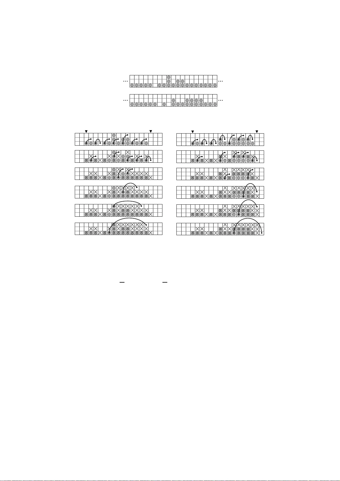
Conserv ed quan tities and g eneralized sol utions of the ultradi screte KdV equatio n Masatak a Kanki 1 , Jun Mada 2 and T etsuji T okihiro 1 1 Graduate sc ho ol of Mathematical Sciences, Univ ersity of T oky o, 3-8- 1 Komaba, T oky o 153 -8914, Japan 2 College of Industrial T ec hnology , Nihon Univ ersit y , 2-11- 1 Shin-ei, Narashino, Chiba 275- 8576, Japan Abstract W e construct generali zed solutions to the ultradiscrete KdV equation, including the so-called negative solition solutions. The method is based on the ultradiscretization of soliton solutions to the discrete KdV equation with gauge t ransformation. The conserved quantities of th e ultradiscrete KdV equation are show n to b e constru cted in a similar wa y to those for the b ox-ball system. 1 In tro duction The ultradiscr ete KdV e q uation: U t +1 n = min " 1 − U t n , n − 1 X k = −∞  U t k − U t +1 k  # (1) was first intro duced as a dy namical equation for the so-ca lled b ox-ball system (BBS)[1, 2]. Since (1) is close d on the binary v alues 0 or 1 , if w e rega rd U t n as the nu mber of balls in the n th box at time step t , and assume the b oundar y condition lim | n |→∞ U t n = 0, it descr ib e s the time evolution of balls in a one dimensio nal ar ray of b oxes. The up dating rule o f the BBS according to (1) ca n b e expr essed as follows. (See figure 1.) • Find all the pairs of a ball and a n adja c en t v aca n t b ox to the r ight o f it, and draw arclines from the ball to the v acant b ox for each of these pair s. • Neglecting the pairs connected b y arclines, find a ll the pairs of a ball and an adjacent v acant b ox to the right o f it and draw arclines in a similar wa y . • Repeat the a bove pro c edure until all the balls are connected to v ac ant boxes, then mov e a ll the ba lls in to the v aca n t boxes co nnected by a r clines. An example of the time evolution pattern is shown in fig ure 2. The consecutive balls b ehave like so litons in the KdV equa tion. F urthermore, when we deno te 1 F i g . 1 F i g . 2 . . . . 1 1 1 1 . . . . . . 1 1 . . . . . . . . . . . . . . . . . . . . . . . . . . . . . . . . . . . 1 1 1 1 . . . . 1 1 . . . . . . . . . . . . . . . . . . . . . . . . . . . . . . . . . . . . . 1 1 1 1 . . 1 1 . . . . . . . . . . . . . . . . . . . . . . . . . . . . . . . . . . . . . . . 1 1 . . 1 1 1 1 1 . . . . . . . . . . . . . . . . . . . . . . . . . . . . . . . . . . . . 1 1 . . . . . 1 1 1 1 . . . . . . . . . . . . . . . . . . . . . . . . . . . . . . . . . . 1 1 . . . . . . 1 1 1 1 . . . . . . . . . . . . . . . . . . . . . . . . . . . . . . . . 1 1 . . . . . . . . 1 1 1 1 . . . . . . . . . . . . . . . . . . . . . . . . . . . . . . . 1 1 . . . . . . . . . . 1 1 1 1 . . … 0 0 0 1 1 1 0 0 1 0 0 1 1 1 0 0 0 0 … 1 1 1 2 2 3 3 … 0 0 0 0 0 0 1 1 0 1 1 0 0 0 1 1 1 0 … t t+1 Figure 1: The up date rules of the BBS. A v aca n t b ox and a b ox with a ball are represented by ‘0 ’ and ‘1’, res pectively . The conser ved quantities are simulta- neously determined. ( q 1 = 3 , q 2 = q 3 = 2.) F i g . 1 F i g . 2 .... 1 1 1 1 ...... 1 1 .... 1 ....................... ........ 1 1 1 1 .... 1 1 ... 1 ...................... ............ 1 1 1 1 .. 1 1 .. 1 ..................... ................ 1 1 .. 1 1 . 1 1 1 .................. .................. 1 1 .. 1 ... 1 1 1 1 .............. .................... 1 1 . 1 ...... 1 1 1 1 .......... ...................... 1 . 1 1 ........ 1 1 1 1 ...... ....................... 1 .. 1 1 .......... 1 1 1 1 .. … 0 0 0 1 1 1 0 0 1 0 0 1 1 1 0 0 0 0 … 1 1 1 2 2 3 3 … 0 0 0 0 0 0 1 1 0 1 1 0 0 0 1 1 1 0 … t t + 1 Figure 2 : A solito nic time e volution patter n of the BBS. The symbol ‘.’ denotes ‘0’. by q 1 the num b er of a r clines drawn in the first step of the up dating rule, b y q 2 one in the seco nd step a nd so o n, we obtain a no nincreasing integer sequence ( q 1 , q 2 , q 3 , . . . ), which is a co ns erved quantit y of the BBS in time[3]. The reaso n why the BBS has these solitonic pro p er ties is understo o d b y the fact that (1 ) is o btained from the KdV equation throug h a limiting pr o cedure, ultradiscretiza tion[4]. The proc e s s inv olved in obtaining (1) from the KdV equa- tion ca n b e explained a s follows. The integrable discrete KdV equation is given in the bilinear form as (1 + δ ) σ t +1 n +1 σ t − 1 n = δ σ t − 1 n +1 σ t +1 n + σ t n σ t n +1 , (2) where ( n, t ) ∈ Z 2 and δ is a discr etization parameter [5]. By putting u t n := σ t n σ t − 1 n +1 σ t n +1 σ t − 1 n , v t n := σ t +1 n σ t − 1 n ( σ t n ) 2 , (3) (2) gives the simultaneous equations (1 + δ ) 1 u t +1 n = δ u t n + 1 v t n , (4) u t +1 n v t n +1 = u t n v t n . (5) 2 F i g . 3 . . . . -1 -2 . . -1 . . . . . . . . . . . -1 -2 . . -1 . . . . . . . . . . . -1 -2 . . -1 . . . . . . . . . . . -1 -2 . . -1 . . . F i g . 4 [ n a g a s o l 1 0 1 1 3 5 . n b ] . . 1 1 1 1 1 . -1 . . 1 1 . - 1 . . . . -1 . . . . . . . . . . . . . . . . . . . 1 2 1 . . . 1 1 - 1 . . . . -1 . . . . . . . . . . . . . . . . . . . -1 . 1 1 1 . . 2 1 . . . . - 1 . . . . . . . . . . . . . . . . . . . - 1 . . . 1 1 - 1 . 1 1 1 1 1 - 1 . . . . . . . . . . . . . . . . . . . -1 . . . . 2 -1 . . . . . 2 1 1 . . . . . . . . . . . . . . . . . . - 1 . . . - 1 2 . . . . . -1 1 1 1 1 1 . . Figure 3: A time evolution pattern of a background solution. When we imp ose the b oundar y condition lim | n |→∞ σ t n = const., then lim | n |→∞ v t n = lim | n |→∞ u t n = 1 from (4) a nd (5) we have (1 + δ ) 1 u t +1 n = δ u t n + n − 1 Y k = −∞ u t +1 k u t k . (6) W e intro duce a pa r ameter ǫ and put δ := e − 1 /ǫ . If there exists a one parameter family of solutions to (6) u t n ( ǫ ), and if the limit lim ǫ → +0 ǫ log u t n ( ǫ ) = : U t n exists, then, using the identities for arbitrary real num b er s a and b lim ǫ → +0 ǫ log  e a/ǫ + e b/ǫ  = max[ a, b ] , lim ǫ → +0 ǫ log  e a/ǫ · e b/ǫ  = a + b , − max[ − a, − b ] = min[ a, b ] , we find that U t n satisfies (1). Recently , (1) has be e n studied without the cons traint o f binar y v alues[6, 7]. One in teresting feature in this extension is tha t there exist ba ckground solutions comp osed of so-ca lled neg ative solitons trav elling a t sp eed one[6]. A typical example of the background solutions is shown in figure 3. F urthermor e, such negative so litons interact nontrivially w ith ordinary solitons a s shown in fig ure 4. A metho d to solve the initial v alue problem for this generalized situatio n is given in Ref.[7]. F rom these pro per ties, the dynamical systems describ ed by (1) in the general se tting a re als o regar ded as integrable cellular automata, just as the BBS. How ever, several impor tant features of integrable cellular auto ma ta hav e not been clarified yet, such as the conserved quantities, the relation to integrable lattice mo dels , extension to the case o f a cyclic b oundar y condition and so on, all of which ar e w ell understo o d in the case of B B S. In this article , we rep or t that a simple transformatio n reveals the underlying integrable structure o f (1) for the generalized states. By this transformatio n, the rela tio n to the B B S and hence to the integrable lattice mo dels , and generaliza tion to a differ ent bo undary condition b ecome a pparent. W e explicitly show how to obtain the conserved quantities and give the expr ession o f g eneral s olutions to (1) where negative solitons and ordinary solitons co exist. 3 F i g . 3 F i g . 4 [ n a g a s o l 1 0 1 1 3 5 . n b ] . . 1 1 1 1 1 . -1 . . 1 1 . -1 . . . . -1 . . . . . . . . . . . . . . . . . . . 1 2 1 . . . 1 1 -1 . . . . -1 . . . . . . . . . . . . . . . . . . . -1 . 1 1 1 . . 2 1 . . . . -1 . . . . . . . . . . . . . . . . . . . -1 . . . 1 1 -1 . 1 1 1 1 1 -1 . . . . . . . . . . . . . . . . . . . -1 . . . . 2 -1 . . . . . 2 1 1 . . . . . . . . . . . . . . . . . . -1 . . . -1 2 . . . . . -1 . . 1 1 1 1 1 . . … 0 0 0 1 2 0 1 0 0 0 0 0 … … 0 0 0 1 2 0 1 0 0 0 0 0 … 0 0 0 0 0 1 2 0 1 0 0 0 … … 0 0 0 0 0 1 2 0 1 0 0 0 Figure 4 : A time evolution pattern in which ne g ative solitons and ordinary solitons co exist. 2 Conserv ed quan tities for states with negativ e solitons W e s tart from the ultra discretization of the coupled equatio ns (4) a nd (5). By putting δ = e − 1 /ǫ and assuming that the limit lim ǫ → +0 ǫ log u t n ( ǫ ) = : U t n , lim ǫ → +0 ǫ log v t n ( ǫ ) =: V t n exist, we obta in the equations U t +1 n = min  1 − U t n , V t n  , (7) V t n +1 = U t n + V t n − U t +1 n . (8) If we imp ose the b oundary condition lim | n |→∞ U t n = lim | n |→∞ V t n = 0 , E qs. (7) and (8) are equiv ale nt to (1). It is easily s een that (7) and (8) are generaliz ed by int ro ducing a p ositive integer constants L a nd C as U t +1 n = U t n + min  L − U t n , V t n  − min  U t n , C − V t n  , (9) V t n +1 = U t n + V t n − U t +1 n . (10) Equations (9) and (10) are known as the ultradiscr ete limit of the mo dified KdV equation and are interpreted as a BBS of b ox c apacity L with carr ier of capa cit y C [8, 9]. A t the sa me time, they represent the a c tio n of the combinatorial R- matrix of an A (1) 1 crystal o n a certain symmetric tensor pro duct r epresentation as long as U t n ∈ { 0 , 1 , · · · , L } a nd V t n ∈ { 0 , 1 , 2 , · · · , C } [10]. Note that Eqs. (9) and (10) are closed under the v a lue s U t n ∈ { 0 , 1 , · · · , L } and V t n ∈ { 0 , 1 , 2 , · · · , C } . Hence the time evolution patterns of the BBS are r egarded as the gro und states of a 2 dimensiona l integrable lattice model at temp era ture 0 and its generaliza - tion has b een inv estigated in detail[11, 12]. When we a llow U t n or V t n in (7) a nd (8) to take nega tive int eger v alues and/or the v alues greater than L or C res pectively , they ar e no long er interpreted as a BBS nor as a realiza tion of the com binatorial R- matrix. F or an arbitra ry initial state including neg ative integer v alues , let M := − min n ∈ Z  U 0 n , V 0 n , L − U 0 n , C − V 0 n  . When we change v ariables ˜ U t n := U t n + M , ˜ V t n := V t n + M , ˜ L := L + 2 M , ˜ C := C + 2 M , then w e find that Eqs. (9) and (10) a re unchanged under this gauge 4 transformatio n[13 ], that is, ˜ U t +1 n = ˜ U t n + min h ˜ L − ˜ U t n , ˜ V t n i − min h ˜ U t n , ˜ C − ˜ V t n i , ˜ V t n +1 = ˜ U t n + ˜ V t n − ˜ U t +1 n . Since these equations ar e closed under the v alues ˜ U t n ∈ { 0 , 1 , · · · , L + 2 M } and ˜ V t n ∈ { 0 , 1 , 2 , · · · , C + 2 M } , a nd initial v alues ˜ U 0 n , ˜ V 0 n belo ng to the sa me sets, we ca n r egard them as equations for a BBS with b ox ca pa city L + 2 M and carrier c apacity C + 2 M , and regar d them a s a rea liz ation of A (1) 1 crystal lattice comp osed of a larg er tensor pro duct r epresentation. Thus we ca n co nclude that Eqs. (9) and (10 ) as well as Eqs. (7) and (8) do not ch ange their mathematical structure even in the cas e wher e the dep endent v ar iable take neg ative in teger v alues. F rom the a b ove argument, we find that we can identify the ultradiscrete K dV equation (1) as a BBS with larger box capacity when its dep endent v ar iables ta ke negative integer v alues. The conser ved quantities of the BBS hav e b een w ide ly inv estig a ted in gener al cases and we can apply the results to this system[11, 1 4]. In [1 1, 1 5], it is shown that the energ y functions which are combinatorially determined, a re conser ved in time, a nd in [14] the path description fo r the conserved quantities is g iven. Here we give another e x pression o f the conserved quantities for (1). Let M := − min n [ U 0 n , V 0 n , 1 − U 0 n ]. Then Eqs . (7) and (8) ar e transformed to the BBS with b ox capacity 1 + 2 M (with infinite carrier capacity). Let the nu mber of balls in the n th b ox b e ˜ U t n . W e co nsider the time evolution starting from the time step t = 0 , and choo se the tw o integers M 0 and N 0 which satisfy the following co nditions. 1. U 0 n = U 1 n = 0 for n ≤ M 0 + 1 and N 0 − 1 ≤ n ( ˜ U 0 n = ˜ U 1 n = M ( n ≤ M 0 + 1 , N 0 − 1 ≤ n )). 2. N 0 − M 0 ≡ 0 (mo d 2). 3. No v a cancy in the N 0 th box is connected by a n arcline in the first s tep of the construction of the conse rved quantities which w e explain be low. The conditions 2, 3 are used to avoid the redundancy of the definition o f c on- served quantities. F or the time step t , from the b oundar y co ndition, there exists tw o integers M t , N t such that U t n = V t n = U t +1 n = 0 for n ≤ M t − 1 and N t + 1 ≤ n ( ˜ U t n = ˜ U t +1 n = M ( n ≤ M t + 1 , N t − 1 ≤ n )). F urthermore we impo se the following co nditions on them. N t − M t ≡ 0 (mo d 2) , M t − M 0 ≡ t (mo d 2) , N t − N 0 ≡ t (mo d 2) . A t each times step t , we consider the boxes with indices from M t to N t . In other words, we neg le ct all the balls in the b oxes n < M t and n > N t . Then, as in the ca se of the BBS with b ox capacity one, w e draw arclines fro m balls to v acancies to determine the v alues of the conser ved q ua nt ities. (See figure 5.) 5 • Draw an arcline from one o f the leftmost balls to one of its near est right v acancies . • Draw an arcline from o ne o f the leftmost balls which are lo cated on the right of the v acancy we hav e drawn the arcline to o ne of its nearest rig ht v acancies . • Rep eat the ab ov e pro cedure until one has dr awn arc lines b etw een all the pairs o f balls and v acancies. Note that if we drew an a rcline to a v acancy at n th b ox, then the ball from which we draw an arcline in the next step is lo ca ted in the box whose index is gr eater than n , and that there must be no arcline starting from a ball in the la st b ox due to the condition 3. Let ˜ q 1 ( t ) be the num b er of a r clines drawn in this step. • Then negle c ting all the b oxes and v ac a ncies which are connected by ar- clines, r ep e at the ab ov e pro cedure and let ˜ q 2 ( t ) b e the n um b er o f ar clines drawn in the seco nd step. • Rep eat the a bove pro ce dur e until all the balls but those in the N t th box are co nnected and le t ˜ q j ( t ) ( j = 3 , 4 , . . . ) b e the num ber of a r clines drawn in the j th steps. • Let q j := ˜ q j ( t ) − 1 2 ( N t − M t ) ( j = 1 , 2 , ..., 2 M ) and q j := ˜ q j ( t ) ( j = 2 M + 1 , 2 M + 2 , . . . ). Note that we o btain the up dated state of the B BS with carrier c apacity C if w e exchange the ba lls with the v a cancies connected to them up to the C th s teps , i.e., if w e exchange the first C X j =1 ˜ q j pairs of balls and v a cancies. Then we find the following pr op osition. Prop ositio n 1 The sequence ( q 1 , q 2 , q 3 , . . . ) does not depend on t . The sta temen t of the prop osition is the direc t consequence of the fact that k X i =1 ˜ q i is equal to the num b er of balls mov ed b y the carrier with capacity k at one time step which is the v alue of k th energ y function[11, 12]. Here we map the system to the BBS with box ca pacity 2 M + 1 in whic h the n umber of balls is finite, that is, the n th b ox is v acant for n ≤ M t − 1 and N t ≤ n . Of course we can make another choice. W e could impos e the condition N t − M t ≡ 1 (mo d 2) o r the condition that a v acancy in the N 0 th b ox is connec ted by an arcline in the first step. This redundancy is cause d by the fact that there ar e essentially four types of finite systems whic h a re equiv alent to this system. Once we de ter mine the type how ever, the s equence ( q 1 , q 2 , . . . ) do es not dep e nd on N t and M t as long as they ar e sufficiently large and, when ther e is no negative soliton q 2 M + j = ˆ q j ( j = 1 , 2 , . . . ), where ˆ q j is the j th conserved quantit y defined in the orig inal BB S. 6 F i g . 5 = 7 , = 5 , = 2 , = 1 , = 1 , = 1 ; $ + , = 7 , $ + , = 5 , $ + , = 2 , $ + , = 1 , $ + , = 1 , $ + , = 1 t t +1 N t M t N t +1 M t +1 t +1 t Figure 5: The sch eme to count the conserved quantities of the BBS with la rger capacities. W e have to cho ose different seq uences of boxes a t time step t and t + 1. F rom this figur e, we hav e ˜ q 1 ( t ) = 7 , ˜ q 2 ( t ) = 5 , ˜ q 3 ( t ) = 2 , ˜ q 4 ( t ) = 1 , ˜ q 5 ( t ) = 1 , ˜ q 6 ( t ) = 1 and ˜ q 1 ( t + 1 ) = 7 , ˜ q 2 ( t + 1 ) = 5 , ˜ q 3 ( t + 1 ) = 2 , ˜ q 4 ( t + 1 ) = 1 , ˜ q 5 ( t + 1 ) = 1 , ˜ q 6 ( t + 1 ) = 1. Since M = 1, N t − M t = 14 and N t +1 − M t +1 = 14, we o btain q 1 = 7 − 14 2 = 0 , q 2 = 5 − 14 2 = − 2 , q 3 = 2 , q 4 = q 5 = q 6 = 1 in b oth time steps. 3 Soliton solutions in teracting with a bac kground state F or the o riginal BBS wher e every box capa city is one and o nly a finite n umber of balls exist, all the solutions ar e pr oved to be constructed by ultradis c r etization from the soliton solutions of the discr e te KdV equation (6) [16]. Although the ultradiscrete KdV equation (1) ov er ar bitrary integers is s hown to b e equiv alent to the B BS with la rger box capacity , the solutions to them can not b e the ultradiscrete limit of soliton solutions to (6), b eca us e the b oundar y condition of the BBS changes such that the n umber of balls b ecomes M for | n | → ∞ . Nevertheless we s hall show that solutions ca n b e constr ucted from the so liton solutions to (6) through ultradis cretization with a n appr opriate scaling limit. Here we treate only the case M = 1. Our metho d for constr ucting the solutio ns is equally applicable to the case M ≥ 2, a ltho ugh the analysis of that case is 7 more elab ora te. The coupled equations for the BBS a re e x plicitly written as U t +1 n = min  3 − U t n , V t n  , (11) V t n +1 = U t n + V t n − U t +1 n , (12) with the b oundary condition lim | n |→∞ U t n = lim | n |→∞ V t n = 1 . (13) F rom (2) and (3), if we put δ = e − L/ǫ ( L ∈ Z + ) and assume that ρ t n := lim ǫ → +0 ǫ log σ t n exists, we find ρ t +1 n +1 + ρ t − 1 n = max  ρ t − 1 n +1 + ρ t +1 n − L , ρ t n + ρ t n +1  . (14) F rom (3), if we put U t n = ρ t n − ρ t − 1 n − ρ t n +1 + ρ t − 1 n +1 , (15) V t n = ρ t n +1 − 2 ρ t n + ρ t n − 1 , (16) they satisfy (11) a nd (1 2 ) for L = 3. Hence we will construct solutions ρ t n of (14) which sa tisfy the bo unda ry conditions (13). First let us consider a state wher e only negative solitons exist. The corr e- sp onding solution is called a background solution [7]. It is a stationar y solution of the form U t n = F ( n − t ) where { F ( k ) } ∞ k = −∞ is a 01 sequence with o nly finite nu mber o f 0s . Let the num ber of 0s b e s + 1 ( s ∈ Z ≥ 0 ), and let b 0 = δ 0 = 0, b i ∈ Z ≥ 0 ( i = 1 , 2 , . . . , s ) a nd δ i ∈ { 0 , 1 } ( i = 1 , 2 , . . . , s ). W e define a 01 sequence { ˜ F ( k ) } ∞ k = −∞ as ˜ F ( k ) =  0 k = − P j i =0 (2 b i + δ i + i ) ( j = 0 , 1 , 2 , . . . , s ) , 1 otherwise . (17) Apparently any background solution F ( k ) can b e expressed as F ( k ) = ˜ F ( k − a ) for some integers a, s, { b i } and { δ i } . The N s oliton solution to (2) is given a s σ t n = 1 + X J ⊆ [ N ] J 6 = φ Y i ∈ J ( − γ i )  1 − p i p i  t  p i + δ 1 + δ − p i  n ! Q i>j,i,j ∈ J ( p i − p j ) 2 Q i,j ∈ J (1 − p i − p j ) , (18) where p i ∈ C and γ i ∈ C ( i = 1 , 2 , . . . , n ) ar e arbitrar y but p i 6 = p j for i 6 = j [4, 5 ]. W e often denote [ k ] := { 1 , 2 , 3 , . . . , k } for a p ositive integer k . T o take the ultradis crete limit, let δ = e − L/ǫ , p i = N i e − P i /ǫ , − γ i = M i e − C i /ǫ ( i = 1 , 2 , . . . , N ) where C i ∈ R , L, P i , N i , M i > 0 and N i 6 = N j , M i 6 = M j for i 6 = j . Then taking the limit lim ǫ → +0 ǫ log σ t n =: ρ t n , we hav e ρ t n = max      0 , max J ⊆ [ N ] J 6 = φ    X i ∈ J ( C i + tP i − n min[ P i , L ]) − X i,j ∈ J i 6 = j min[ P i , P j ]         . (19) 8 F or L = 1, w e find that U t n and V t n satisfy (7) a nd (8), and hence (1) . In particular, if P i ∈ Z + , C i ∈ Z , (19) g ives an N so liton so lution o f the or iginal BBS. W e ar e, howev er , concerned with Eqs. (11) and (12) with the b ounda ry con- dition (13). Herea fter we put L = 3 a nd prepa re several s y m b ols and no tations: l : = s X i =1 δ i , δ s +1 ≡ s − l + 1 (mo d 2) , l ′ := l + δ s +1 , K : = l + s X i =1 b i , B i := i X j =0 b j , ∆ i := i X j =0 δ i , W e also a ssume that δ i = 1 for i = m 1 , m 2 , . . . , m l (1 ≤ m 1 < m 2 < · · · < m l ≤ s ), and m l +1 := s + 1. Let us consider an n ∞ soliton so lution ( n ∞ ≫ 1) of the form (19). W e assume that P i = 2 (1 ≤ i ≤ n ∞ − l ′ ) and P ′ i := P i + n ∞ − l ′ = 1 (1 ≤ i ≤ l ′ ). The phase s a re chosen as C i =    1 (1 ≤ i ≤ n 0 ) , − 2 j + 1 ( n 0 + B j − 1 + 1 ≤ i ≤ n 0 + B j ( j = 1 , 2 , ..., s )) , − 2 s − 1 ( n 0 + B s + 1 ≤ i ) , C ′ i ≡ C i + n ∞ − l ′ := − ( m i − i ) ( i = 1 , 2 , ..., l ′ ) . Then we find ρ t n = max 0 ≤ k 1 ≤ n ∞ − l ′ 0 ≤ k 2 ≤ l ′ " k 1 X i =1 ( C i − 2 ( n − t )) + k 2 X i =1 ( C ′ i − ( n − t )) − 2 k 1 ( k 1 − 1 ) − k 2 ( k 2 − 1 ) − 2 k 1 k 2 # = max − n 0 ≤ k 1 ≤ n ∞ − l ′ − n 0 0 ≤ k 2 ≤ l ′   − (2 k 1 + k 2 )( n − t + 2 n 0 ) + k 1 X i =1 ′ ¯ C i + k 2 X i =1 C ′ i − 2 k 1 ( k 1 − 1 ) − k 2 ( k 2 − 1 ) − 2 k 1 k 2 # − 2 n 0 ( n − t + 2 n 0 ) + 2 n 2 0 + 3 n 0 , where ¯ C i := C n 0 + i , k X i =1 ′ ¯ C i :=      k X i =1 ¯ C i ( k ≥ 1) , k ( k ≤ 0) . It is o bvious that if ρ t n is a so lution to (14), ρ t + c n + b + at + f ( n ) is also a s o lution for an a rbitrary function f ( n ) and ar bitrary v alues a, b and c . Hence we find 9 that ρ t n = ρ n 0 ,n ∞ ( n − t ) is a so lution to (14), where ρ n 0 ,n ∞ ( x ) = max − n 0 ≤ k 1 ≤ n ∞ − l ′ − n 0 0 ≤ k 2 ≤ l ′   − (2 k 1 + k 2 ) x + k 1 X i =1 ′ ¯ C i + k 2 X i =1 C ′ i − 2 k 1 ( k 1 − 1 ) − k 2 ( k 2 − 1 ) − 2 k 1 k 2 # . Since n 0 , n ∞ are larg e but ar bitrary po sitive integers, the limit ρ F ( x ) := lim n 0 →∞ lim n ∞ →∞ ρ n 0 ,n ∞ ( x ) = ma x k 1 ∈ Z 0 ≤ k 2 ≤ l ′   − (2 k 1 + k 2 ) x + k 1 X i =1 ′ ¯ C i + k 2 X i =1 C ′ i − 2 k 1 ( k 1 − 1 ) − k 2 ( k 2 − 1 ) − 2 k 1 k 2 # (20) is also a solution to (14). When we rewr ite in (1 4) a s max r ∈ Z   − rx + max 0 ≤ k 2 ≤ l ′ 2 k 1 + k 2 = r   k 1 X i =1 ′ ¯ C i + · · ·     and using the rela tions s uch as a 0 + a 2 ≥ 2 a 1 − → ma x[ − 2 x + a 2 , − x + a 1 , a 0 ] = max[ − 2 x + a 2 , a 0 ] Eq. (20) can b e simplified as shown in the Prop osition 2 b elow. Fir st let us define some symbols and notatio ns . C T := s X j =1 (2 j − 1) b j + l X j =1 ( m j − j ) , Q 0 := C T + K ( K − 1) + ( K − l )( K − l − 1) S 1 := { m 1 , m 2 , . . . , m l } , S 0 := [ l ] \ S 1 , I := [2 K − l ] \ ¯ I ¯ I := n m ∈ [2 K − l ]    m = 2 B i − 1 + ∆ i − 1 + 2 k i + 1 , k i = 0 , 1 , . . . , b i − 1 − 1 , i ∈ S 0 o The quantit y Θ r is defined for r ∈ I a s • If i ∈ S 0 and 2 B i − 1 + ∆ i − 1 + 2 ≤ r ≤ 2 B i + ∆ i , then putting r = 2 B i − 1 + ∆ i − 1 + 2 k ( k ∈ Z ), Θ r := i − 1 X j =1 " (2 j − 1) b j + ( j − j X µ =1 δ µ ) δ j # + (2 i − 1) k + ( B i − 1 + k + ∆ i − 1 )( B i − 1 + k + ∆ i − 1 − 1 ) + ( B i − 1 + k )( B i − 1 + k − 1 ) . (21) 10 • If i ∈ S 1 , 2 B i − 1 + ∆ i − 1 + 1 ≤ r ≤ 2 B i + ∆ i and r = 2 B i − 1 + ∆ i − 1 + 2 k ( k ∈ Z ), then Θ r is given by (21). • If i ∈ S 1 , 2 B i − 1 + ∆ i − 1 + 1 ≤ r ≤ 2 B i + ∆ i and r = 2 B i − 1 + ∆ i − 1 + 2 k + 1 ( k ∈ Z ), then Θ r := i − 1 X j =1 (2 j − 1) b j + i X j =1 ( j − j X µ =1 δ µ ) δ j + (2 i − 1 ) k + ( B i − 1 + k + ∆ i )( B i − 1 + k + ∆ i − 1 ) + ( B i − 1 + k )( B i − 1 + k − 1 ) . (22) Prop ositio n 2 ρ F ( x ) := ma x h ρ ( − ) F ( x ) , ρ (0) F ( x ) , ρ (+) F ( x ) i , (23) where ρ ( − ) F ( x ) := ma x k ≥ 0 k ∈ Z [(2 x − 1) k − 2 k ( k + 1)] , (24) ρ (+) F ( x ) :=      max q ≥ 1 q ∈ Z [ − (2 K − l + 2 q ) x − q (2 q + 4 K − 2 l + 2 s − 1) − Q 0 ] ( δ s +1 = 0) , max q ≥ 1 q ∈ Z h − (2 K − l + q ) x − ( q − 1)  q 2 + 2 K − l + s  − s − Q 0 i ( δ s +1 = 1) , (25) ρ (0) F ( x ) := max 1 ≤ r ≤ 2 K − l r ∈ Z h ρ ( r ) ( x ) i , (26) and the function ρ ( r ) ( x ) is given a s ρ ( r ) ( x ) :=  − rx − Θ r r ∈ I , 0 r / ∈ I . F rom (15), if we define U F ( x ) := ρ F ( x + 2) − 2 ρ F ( x + 1) + ρ F ( x ) , (27) U t n = U F ( n − t ) gives a s olution to (11) and (12). By using the fact that ρ F ( x ) is a contin uo us and co nv ex piecewis e linear function, and by calcula ting the intersection p oints of each linear functions app eare d as linear pieces in the function ρ F ( x ), we o btain the explicit for m of U F ( x ). Let us define t i ( x ) ( i = 11 1 , 2 , ... ) as t 1 ( x ) :=    x + 2 ( − 2 ≤ x ≤ − 1) , − x ( − 1 ≤ x ≤ 0) , 0 otherwise , t 2 ( x ) :=    2 x + 5 ( − 5 / 2 ≤ x ≤ − 3 / 2) , − 2 x − 1 ( − 3 / 2 ≤ x ≤ − 1 / 2) , 0 otherwise , t 2 k +1 ( x ) := 2 k X i =0 t 1 ( x + i ) , t 2 k ( x ) := k − 1 X i =0 t 2 ( x + 2 i ) . By straightforward but a little tedious calculation, we find U F ( x ) = U ( − ) F ( x ) + U (0) F ( x ) + U (+) F ( x ) , (28) where U ( − ) F ( x ) := ∞ X k =1 t 2 ( x − 2 k − 1 ) , (29) U (+) F ( x ) :=            ∞ X k =0 t 2 ( x + K + s + 2 k ) ( δ s +1 = 0) , ∞ X k =0 t 1 ( x + K + s + k ) ( δ s +1 = 1) , (30) U (0) F ( x ) := s X i =1 t 2 b i + δ i ( x + 2 B i − 1 + ∆ i − 1 + i − 1) . (31 ) An example of the function U F ( x ) is shown in figure 6. Compar ing these e x- pressions with ˜ F ( k ), we find that U F ( k ) = ˜ F ( k ) fo r k ∈ Z . Thus w e have prov ed the following pr op osition. Prop ositio n 3 It holds that U F ( k ) = ˜ F ( k ) for k ∈ Z . F urthermor e, compa ring ˜ F ( k ) with the co nserved q uantit ies { q j } defined in the previous section, we ha ve the following pr op osition. Prop ositio n 4 The num b er of negative so litons is equa l to − q 1 − q 2 , i.e., s + 1 = − q 1 − q 2 , and q 1 − q 2 is the num ber of so litons with amplitude 1 which is used to construct the background s olution, i.e., q 1 − q 2 = l ′ . Next we consider the s olutions in whic h m ordinary solitons exist in a back- ground state. Since N s oliton solutions are given by (1 9) and the parameter s 12 F i g . 6 b _1 = 1 , ¥ d e l t a _1 = 1 , b _2 = 2 , ¥ d e l t a _2 = 0 = F i g . 7 ¥ h a t { P } _1 = 4 , ¥ h a t { C } _1 = - 7 , ¥ h a t { P } _2 = 7 , ¥ h a t { C } _2 = - 5 , b _1 = 2 , ¥ d e l t a _1 = 0 , b _2 = 1 , ¥ d e l t a _2 = 1 . . 2 2 2 2 2 . 0 . . 2 2 . 0 . . . . 0 . . . . . . . . . . . . . . . . . . . 2 3 2 . . . 2 2 0 . . . . 0 . . . . . . . . . . . . . . . . . . . 0 . 2 2 2 . . 3 2 . . . . 0 . . . . . . . . . . . . . . . . . . . 0 . . . 2 2 0 . 2 2 2 2 2 0 . . . . . . . . . . . . . . . . . . . 0 . . . . 3 0 . . . . . 3 2 2 . . . . . . . . . . . . . . . . . . 0 . . . 0 3 . . . . . 0 . . 2 2 2 2 2 . . 1 1 1 1 0 1 1 1 1 0 1 1 1 0 1 1 1 1 1 1 1 1 2 1 Figure 6: An example of ˜ F ( x ) a nd U F ( x ). The parameters are b 1 = 1 , δ 1 = 1 , b 2 = 2 , δ 2 = 0. for the ba ckground solution ar e a lready known, we hav e o nly to add new pa- rameters { ˆ P i } m i =1 ( ∀ i ˆ P i ≥ 3) and { ˆ C i } m i =1 . When we deno te the set of indices for a background so lution B , then the solution is given b y ρ t n = max J 1 ⊆ [ m ] ,J 2 ⊆B " X i ∈ J 1 ( − min[3 , ˆ P i ] n + ˆ P i t + ˆ C i ) + X i ∈ J 2 ( − P i ( n − t ) + C i ) − X i 6 = j,i,j ∈ J 1 min[ ˆ P i , ˆ P j ] − X i 6 = j,i,j ∈ J 2 min[ P i , P j ] − 2 X i ∈ J 1 ,j ∈ J 2 min[ ˆ P i , P j ] # = max J 1 ⊆ [ m ] ,J 2 ⊆B " X i ∈ J 1 ( − 3 n + ˆ P i t + ˆ C i ) + X i ∈ J 2 ( − P i ( n − t ) + C i ) − X i 6 = j,i,j ∈ J 1 min[ ˆ P i , ˆ P j ] − X i 6 = j,i,j ∈ J 2 min[ P i , P j ] − 2 X j ∈ J 2 | J 1 | P j # = max J 1 ⊆ [ m ]   X i ∈ J 1 ( − 3 n + ˆ P i t + ˆ C i ) − X i 6 = j,i,j ∈ J 1 min[ ˆ P i , ˆ P j ] + max J 2 ⊆B   X i ∈ J 2 ( − P i ( n − t + 2 | J 1 | ) + C i ) − X i 6 = j,i,j ∈ J 2 min[ P i , P j ]     . Here we used the a bbreviation max J ⊆A [ · · · ] ≡ ma x  0 , max J ⊆A ,J 6 = φ [ · · · ]  . Therefore we o btain the following theorem. Theorem 1 The s olution to (14) r epresenting the interaction of m soliton solutio ns with the background given by (23) , has the expressio n: ρ t n = max J ⊆ [ m ]    X i ∈ J ( − 3 n + ˆ P i t + ˆ C i ) − X i 6 = j i,j ∈ J min[ ˆ P i , ˆ P j ] + ρ F ( n − t + 2 | J | )    . (32) 13 F i g . 6 b _1 = 1 , ¥ d e l t a _1 = 1 , b _2 = 2 , ¥ d e l t a _2 = 0 F i g . 7 ¥ h a t { P } _1 = 4 , ¥ h a t { C } _1 = - 7 , ¥ h a t { P } _2 = 7 , ¥ h a t { C } _2 = - 5 , b _1 = 2 , ¥ d e l t a _1 = 0 , b _2 = 1 , ¥ d e l t a _2 = 1 . . 2 2 2 2 2 . 0 . . 2 2 . 0 . . . . 0 . . . . . . . . . . . . . . . . . . . 2 3 2 . . . 2 2 0 . . . . 0 . . . . . . . . . . . . . . . . . . . 0 . 2 2 2 . . 3 2 . . . . 0 . . . . . . . . . . . . . . . . . . . 0 . . . 2 2 0 . 2 2 2 2 2 0 . . . . . . . . . . . . . . . . . . . 0 . . . . 3 0 . . . . . 3 2 2 . . . . . . . . . . . . . . . . . . 0 . . . 0 3 . . . . . 0 . . 2 2 2 2 2 . . 1 1 1 1 0 1 1 1 1 0 1 1 1 0 1 1 1 1 1 1 1 1 2 1 Figure 7 : A solutio n U t n given b y (32). Here U t n = ρ t n − ρ t − 1 n − ρ t n +1 + ρ t − 1 n +1 . The symbol ‘.’ denotes ‘1’. The par ameters are ˆ P 1 = 4 , ˆ C 1 = − 7 , ˆ P 2 = 7 , ˆ C 2 = − 5 , b 1 = 2 , δ 1 = 0 , b 2 = 1 , δ 2 = 1. When w e make gag e transfo r mation a s U t n − 1 → U t n , this time evolution patter n coincides with that of figur e 4 . The m ulti-soliton solutions with a background is also given by Y. Nak ata in an algebraic form (nested maximizatio n) with the ultaradiscr ete vertex oper ators[1 8 ]. So far we do no t find the ex act corres po ndence b etw een our solution (32) and his formula. F rom (32), we find that the phase s hift of negative so lito ns after co llision of an o rdinary solito n is − 2. An example of a time evolution pattern is shown in figure 7. Since the solution (32) s hows that the o rdinary solitons mov e freely for t ≫ 1 as those in the B B S with box capacity o ne, comparing with the construction of conserved qua nt ities, we find the following prop osition[1 7]. Prop ositio n 5 F or a solution to (1) determined by (32 ) , let Y be the Y o ung diagr am cor re- sp onding to the par tition ( q 3 , q 4 , q 5 , · · · ) constituted by the co nserved quantities, that is, the length of its i th column o f Y is q i +2 . Then, the length of j th row in Y is equa l to ˆ P j − 2 . 4 Concluding remarks W e constr uc ted the conserved quant ities of the ultr adiscrete KdV equa tion (1) with nega tive so litons by using the transfor ma tion to the BB S with larger b ox capacities. The s olutions to (1) in which neg ative solitons and ordinary solitons co exist a re also obtained as the so lutions to this extended BB S. In the BBS with b ox capa city one, every state is obtained by ultradiscr etization of a soliton solution of the discre te KdV e q uation, and using this fact, initial v a lue problem is solved with elementary com binatorial metho ds. W e co njecture that this fact also holds for the extended BBS and can b e used to solve the initial v alue problems. In vestigating this co njecture is a problem we wish to address in the future. Ac kn o wledgemen t The a uthors w is h to thank Pro fessors Atsushi Nag ai and Ralph Willo x for useful discussions and comments. 14 References [1] D. T ak a hashi and J. Satsuma 19 9 0 “A soliton cellular automa ton”, J. Phys. So c. Jpn. 59 , 351 4–351 9 [2] D. T ak ahashi 1993 “O n some soliton sy stems defined by us ing b oxes and balls ”, Pr o c. Int. Symp. on N online ar The ory and its Applic ations (NOL T A’93 ), 55 5–558 [3] M. T orii, D. T ak aha shi and J. Satsuma 1990 “Combinatorial r epresentation of in v aria nts of a soliton cellular automaton” , Physic a D92 , 209– 220 [4] T. T okihiro, D. T ak a hashi, J. Ma tsukidaira and J. Satsuma 199 6 “F rom soliton equa tions to in tegrable ce llula r a utomata thro ug h a limiting pro ce- dure”, Phys. R ev. L ett. 76 , 3247–3 2 50 [5] R. Hirota, S. Tsujimoto and T. Ima i 1992 “Difference Scheme of Soliton Equations” , F u tur e dir e ctions of nonline ar dynamics in physic al and bio- lo gic al systems N A TO A dv. Sci. Inst. Ser. B: Phys. 312 , Plenum , 7–1 5 [6] R. Hirota 2 009 “ New So lutio ns to the Ultradiscrete Soliton E quations”, Stud. A ppl. Math. 122 , 361–3 76 [7] R. Willox, Y. Nak ata, J. Satsuma, A. Ramani a nd B. Gr ammaticos 20 1 0 “Solving the ultradiscrete KdV equa tion”, J. Phys. A: Math. The or. 43 , 48200 3, 7pp [8] D. T a k ahashi and J. Matsuk ida ira 1 997 “B ox a nd ball s y stem with a carr ier and ultradiscrete mo dified K dV equation”, J. Phys. A: Math. Gen. 3 0 , L733–7 39 [9] M. Murata, S. Iso jima, A. Nob e a nd J . Satsuma 200 6 “E xact s olutions for discrete and ultradiscrete mo dified K dV equatio ns a nd their relation to box-ball systems”, J. Phys. A: Math. Gen. 39 , L27–34 [10] A. Nak ayashiki and Y. Y ama da 1997 “Ko stk a p oly nomials a nd ener gy func- tions in solv able lattice mo dels”, Sele cta Mathematic a, New Ser. 3 , 547–59 9 [11] K. F ukuda, M. Ok ado and Y. Y amada 2000 “Ene r gy functions in b ox ball systems”, Int. J. Mo d. Phys. A 15 , 137 9–139 2 [12] G. Hatay ama, K. Hik ami, R. Inoue, A. Kuniba, T. T ak agi and T. T okihiro 2001 “The A (1) M automata re lated to crystals of symmetric tenso rs”, J. Math. Phys. 42 , 274–3 08 [13] This transformation was indep endently found out by C . Gilson, A. Nagai and J. Nimmo. (priv ate co mm unication). [14] J. Mada , M. Idzumi and T. T okihir o 200 5 “Path des c r iption o f conserved quantities of genera lized p erio dic box-ball s ystems”, J. Math. Phys. 4 6 , 02270 1, 19pp [15] K. F ukuda 2 0 04 “Box-ball sy stems and Robinson-Schensted-Knuth corre- sp ondence”, J. Algebr aic Combin. 1 9 , 67–89 15 [16] J. Mada, M. Idzumi a nd T. T okihiro 20 08 “The b ox–ball s ystem and the N -soliton solution of the ultradiscr ete KdV equation”, J . Phys. A: Math. The or. 41 , 175 207, 2 3pp [17] D. Y o s hihara, F. Y ura and T. T ok ihir o 200 3 “F undamental Cycle o f a Periodic Box-Ball Sys tem” , J. Phys. A: Math. Gen. 36 , 99– 121 [18] Y. Nak a ta 201 0 “V ertex op erato rs and background solutions for ultradis- crete soliton equations” , Do ctor Thesis, Un iversity of T okyo 16