On the reconstruction of block-sparse signals with an optimal number of measurements

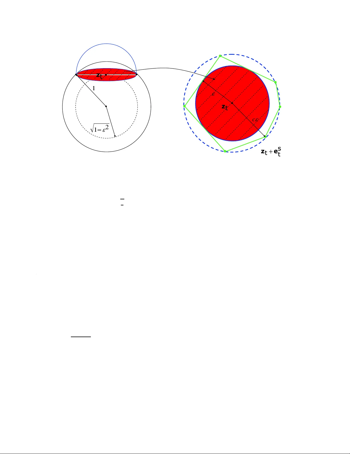
On the r econstruc tion of block-spa rse signals with an optim al number of measurements Mihailo Stojnic, F arzad P arvar esh a nd Babak Hassib i Californi a Institu te of T echnology 1200 East Californi a, Pasaden a, CA, 9112 5, USA. { mihailo , farzad , hassibi } @systems.caltec h.edu Abstract Let A be a n M b y N matrix ( M < N ) which is an insta nce of a re al ra ndom Gau ssian ensemble. In compr essed sensin g w e ar e inter ested in finding the spars est solution to the system of equations A x = y for a given y . In gen eral, whenev er the sparsit y of x is smaller than half the dimension of y then with overwh elming pr obab ility ove r A the spar sest solution is unique and can be foun d by an e xhaust ive sear c h over x with an expo nential time comple xity for any y . The r ecent work of Cand ´ es, Donoho, and T ao shows that minimization of the ℓ 1 norm of x subj ect to A x = y r esults in the sparsest solution pr ovided the sparsity of x , say K , is smaller than a certa in thr esh old for a given number of m easur ements. Specifi cally , if the dimension of y appr oache s the dimension of x , the spar sity of x shoul d be K < 0 . 23 9 N . Her e, we consider the case wher e x is d -bloc k sparse , i.e., x consists of n = N / d block s w her e each bloc k is either a zer o vector or a nonzer o vector . Ins tead of ℓ 1 -norm r elax ation, we consid er the followin g r elaxa tion mi n x k X 1 k 2 + k X 2 k 2 + . . . + k X n k 2 , subjec t to A x = y ( ⋆ ) wher e X i = ( x ( i − 1 ) d + 1 , x ( i − 1 ) d + 2 , . . . , x id ) for i = 1 , 2, . . . , N . Our main r esult is that as n → ∞ , ( ⋆ ) find s the spar sest solution to A x = y , with overwhelming pr obability in A , for any x whose bloc k spar sity is k / n < 1 / 2 − O ( ε ) , pr o vided M / N > 1 − 1 / d , and d = Ω ( l o g ( 1 / ε ) / ε ) . The re laxation given in ( ⋆ ) can be solved in polyno mial time using semi-de finite pr o gramming . 1. Intr oduction Let A be an M by N instance of the real random Gaussia n ensemble and x be an N dimensional signa l from R N with sparsity K , i.e., only K elements of x are nonzero. Set y = A x which is an M dimension al vector in R M . In compre ssed sensin g y is called the measur ement vector and A the G aussia n measur ement matrix. Compressed sensin g has applicatio ns in man y differe nt fields such as data mining [14] , erro r-co rrecting codes [12, 16, 18], DN A microarra ys [13, 33, 34], astrono my , tomogr aphy , digita l photog raphy , and A/D con v erters. In general, when K ≪ N one can hope that y = A x is unique for larg e enoug h M which is much smaller than N . In ot her wor ds, inste ad of sensin g an N dimensional signa l x with sparsity K we can measure M random lin ear functi onals of x where M ≪ N and find x by so lving the under -dete rmined system of equati ons y = A x with the ext ra condition that x is K sparse. T he recon structio n can be presen ted as the follo wing optimization problem: mi n x k x k 0 subjec t to A x = y (1) 1 where the ℓ 0 norm or the Hamming norm is the number of nonze ro elements of x . Define α d e f = M / N and β d e f = K / N . In [15], the authors sho w that if β > 1 / 2 α then for any measurement m atrix A one can constr uct diffe rent K sparse signals x 1 and x 2 such that A x 1 = A x 2 . In addition, if β 6 1 / 2 α then there e xists an A such that t he K sparse solutio n to y = A x is unique for an y y ; spec ifically , for random Gauss ian measuremen ts the uniqu eness property holds w ith overwhe lming probability in the choice of A . Howe v er , the recons truction of x for a gi ve n y can be cumbersome. O ne of the fundamen tal questio ns in compressed sensin g is whether one can ef ficient ly recov er x using an optimal number of measurements . 1.1. P rior work A nai ve exha usti ve se arch can r econstruc t the K sp arse solution x to th e systems o f e quations y = A x with O  ( N K ) M 3  comple xity . Recently , Cand ´ es, Romber g, T ao and Donoho [1 0, 11, 30], sho w that the ℓ 0 optimiza tion can be relax ed to ℓ 1 minimizatio n if the sparsity of the signal is K = O ( M / lo g ( N / M ) ) . In this case, the sparse signal is the soluti on to the follo wing ℓ 1 norm optimizat ion with high probabi lity in the choice of A : mi n x k x k 1 subjec t to A x = y (2) This optimiza tion can be solv ed efficien tly using linear programmin g. Faster al gorithms were dis cov ered in [1–3, 35]. For a comp rehensi ve list of papers and results in compressed sensing please check [4]. Donoho and T anner [5, 7, 8] determined the region ( α , β ) for which the ℓ 1 and ℓ 0 coinci de under Gauss ian measuremen ts for ev ery (or almost ev ery) K -sparse ve ctor x . From a refinement o f their resu lt gi ven in [4 5], when β approa ches α the sparsity has to be smaller than 0 . 2 39 N . Notice that, ideally , one should be able to recov er the signal if the spar sity is less than 1 / 2 N . W e hav e to mention that with V andermo nde measurements we can reco ver the sparse signa l with optimal number of measurements effici ently [15]. Howe ver , it is not clear whether the resul ting algorithms (which are v ariations of reco vering a measure from its moments) are rob ust with respect to imperfecti ons, such as noise [9, 27 – 29]. Also, results similar to thos e vali d for Gaussia n m atrice s A hav e been establ ished for se vera l dif ferent ensembles , e.g., Fourier (see e.g., [11]). In this paper , we will focus on dev elopin g rob ust efficient algo rithms that work for Gaus sian measurements. 1.2. Ou r main result W e consider the reconstru ction of block-sparse signal s from their random measurement s. A signal of dimension N which consist s of n blocks of size d = N / n is k sparse if only k blocks of the signal out of n are nonzer o. Such signals aris e in variou s appl ications, e.g., DN A microarra ys, equalizatio n of spa rse commun ication chann els, magneto encephal ography etc. (see e.g., [3 3, 34, 36, 39– 41] and the references there in). W e measu re the signa l with a m d × nd random G aussia n matrix y = A x . More on a scenar io similar to this one the interested reader can find in e.g. [36–38, 42, 44 ]. Using the ℓ 1 relaxa tion for reconstr ucting x does not explo it the fact that the signal is block- sparse, i.e. t hat the nonze ro entries occur in consecuti v e positions . Instead, differe nt techniques were used throug hout the litera ture. In [36 ] the authors adap t standa rd orthog onal matching pu rsuit algo rithm (use d normal ly in case k = 1 ) to the block -sparse case. In [37, 38, 42, 43] the authors use certai n con v ex o r non -con vex relaxatio ns (mostly dif ferent from the standard ℓ 1 ) and discuss their performances . Genera lization of the block- sparse prob- lem to the case when the number of blocks is infinite was considere d in the most recent paper [44]. In this paper we cons ider the follo wing con v ex relaxatio n for the recov ery of x : mi n x k X 1 k 2 + k X 2 k 2 + · · · + k X n k 2 , subjec t to A x = y (3) where X i = ( x ( i − 1 ) d + 1 , x ( i − 1 ) d + 2 , . . . , x id ) , for i = 1 , 2 , . . . , n . W e will analyz e its theore tical performance and sho w that for a large enough d , indep endent of n , if α approa ches one, β can approach 1 / 2 and the optimiz ation of 2 (3) will giv e the unique sparse soluti on with ov erwhelming probability ove r the choice of A for any y . W e will also briefly ou tline ho w (3) can be po sed as a semi-definite prog ram and there fore solved ef ficiently in polynomial time by a host of numerical methods. Furthermor e, we will demon strate ho w (3) can be adapted for practical consid erations . Numerical results that we will present indica te that in practice a modified ve rsion of (3) (gi ven in Section 4) will e ven for moderate v alues o f d be able t o reco ver mos t of the signals with spars ity fairly close t o the number of measurements. Before proceed ing fur ther we state the main result of this work in the follo wing theorem. Theor em 1 . Let A be an m d × nd matrix. Further , let A be an instance of the ran dom Gaussia n ensembl e. Assume that ǫ is a small posi tive number , i.e., 0 < ǫ ≪ 1 , d = Ω ( l o g ( 1 / ǫ ) / ǫ ) , α > 1 − 1 / d , and β = 1 / 2 − O ( ǫ ) . Also, assume that n tends to infin ity , m = α n , and the bloc k-s parsit y of x is smaller than β n . Then, with overwhe lming pr obability , any d -bloc k spars e signal x can be r econs tructed effi ciently fr o m y = A x by solvi ng the optimizatio n pr oblem (3). Our proof techniqu e does not use the restricted isometry pro perty of the measu rement m atrix A , intr oduced in the work of C and ´ es and T ao [11] and further discus sed in [17], nor does it rely on the k -neigh borliness of the projec ted polytopes presen ted in the work of Donoho and T anner [5, 7, 8, 19]. Instead, we look at the null-spa ce of th e measurement matrix A and use a ge neraliza tion of a neces sary and suf ficient condition gi ven in [ 31] for the equi v alence of (1) and (3). W e are able to use some probabil istic argumen ts to sho w that, for a random Gaussian measure ment matrix, (4) gi ven belo w holds with ov erwhelming probability . In our proof w e use a union bound to upper bound the probab ility that (4) fails ; this make s our bou nd loose for α less than one. W e expe ct to get sharp thresho lds for other value s of α by generaliz ing the idea of looking at the neighbo rliness of randomly projected simplices presen ted in [5, 7, 8]. Howe v er , for relaxation in (3 ) instead of simplice s w e hav e to work with the con vex hull B of n d -dimensional spheres. Specifically , one wou ld need to co mpute the pro bability that a rand om h -dimension al af fine plane that passes through a point on the boundary of B w ill be insid e the tangent cone of that gi ven poin t. Solving this prob lem seems to be rather dif ficult. 2. Null-space characterization In this section we intro duce a necess ary and suf ficient condition on the measurement matrix A so that the optimiza tions of (1) and (3) are equi v alent for all k -block spars e x . (see [24–26, 31 ] for v ariation s of this result). Through out the paper we set K to be the set of all subsets of size k of { 1 , 2, . . . , n } and by ¯ K we m ean the complemen t of the set K ⊂ K with respect to { 1 , 2, . . . , n } , i.e., ¯ K = { 1 , 2, . . . , n } \ K . Theor em 2 . Assume th at A is a dm × dn measur ement matrix , y = A x a nd x is k -blo ck sparse . Then (3) coinci des with the solutio n of (1) if and only if for all nonzer o w ∈ R dn wher e A w = 0 and all K ∈ K ∑ i ∈ K || W i || 2 < ∑ i ∈ ¯ K || W i || 2 (4) wher e W i = ( w ( i − 1 ) d + 1 , w ( i − 1 ) d + 2 , . . . , w id ) , for i = 1 , 2 , . . . , n . Pr oof . The proo f goes along the same line as the proofs in [24–26, 31] . The only dif ference is that each com- ponen t of the ve ctor is now replaced by the two norm of the sub vecto r . First w e prove that if (4) is satisfied then the solution of (3) coinci des with the soluti on (1). Let ¯ x be the solution of (1) and let ˆ x be the solution of (3). Further , let ¯ X i = ( ¯ x ( i − 1 ) d + 1 , ¯ x ( i − 1 ) d + 2 , . . . , ¯ x id ) , for i = 1 , 2 , . . . , n and ˆ X i = ( ˆ x ( i − 1 ) d + 1 , ˆ x ( i − 1 ) d + 2 , . . . , ˆ x id ) , for 3 i = 1 , 2, . . . , n . Set K to be the support of ¯ x , then we can write n ∑ i = 1 || ˆ X i || 2 = n ∑ i = 1 || ˆ X i − ¯ X i + ¯ X i || 2 = ∑ i ∈ K || ˆ X i − ¯ X i + ¯ X i || 2 + ∑ i ∈ ¯ K || ˆ X i − ¯ X i + ¯ X i || 2 = ∑ i ∈ K || ˆ X i − ¯ X i + ¯ X i || 2 + ∑ i ∈ ¯ K || ˆ X i − ¯ X i || 2 > n ∑ i = 1 || ¯ X i || 2 − ∑ i ∈ K || ˆ X i − ¯ X i || 2 + ∑ i ∈ ¯ K || ˆ X i − ¯ X i || 2 . (5) Since ¯ x − ˆ x lies in the null-space of A , we hav e ∑ i ∈ K || ˆ X i − ¯ X i || 2 < ∑ i ∈ ¯ K || ˆ X i − ¯ X i || 2 . Thus, (5 ) implies ∑ n i = 1 || ˆ X i || 2 > ∑ n i = 1 || ¯ X i || 2 , which is a contradic tion. Therefore, ¯ x = ˆ x . Now we pro ve the con verse. Assume (4) does not hold. Then there exi sts w ∈ R nd , A w = 0 , w = ( w 1 w 2 ) , w 1 ∈ R kd , w 2 ∈ R ( n − k ) d such that w 1 is k -block sparse and ∑ i ∈ K || W i || 2 6 ∑ i ∈ ¯ K || W i || 2 , where K is the suppor t of w 1 . T ake x = ( w 1 0 ) and y = A x . Since w is in the null-s pace of A , y = A ( 0 − w 2 ) . Therefore we ha ve found a signal ( 0 − w 2 ) which is not k -bloc k sparse and has smaller norm than the k -block sparse ( w 1 0 ) . Remark. W e need not to check (4) for all subsets K ; checki ng the subset with the k large st (in two norm) blocks of w is suf ficient . Howe ve r , the form of Theorem 2 will be more con venient for our subsequent analysis. Let Z be a basis of the null space of A, so that an y d n dimensional vecto r w in the the null-spa ce of A can be repres ented as Z v where v ∈ R d ( n − m ) . For an y v ∈ R d ( n − m ) write w = Z v . W e split w into blocks of size d , W i = ( w ( i − 1 ) d + 1 , w ( i − 1 ) d + 2 , . . . , w id ) , for i = 1 , 2, . . . , n . Then, the c ondition (4) of Theorem 2 is equi v alent to ∑ i ∈ K W i 6 ∑ i ∈ ¯ K W i , for any v ∈ R d ( n − m ) and K ∈ K , where w = Z v . (6) W e denote by I v the ev ent that (6) happens. In the follo wing we find an upper boun d on the probabil ity that I v fail s as n tends to infinity . W e will sho w that for certain va lues of α , β , and d this proba bility tends to zero. Lemma 3 . L et A ∈ R dm × d n be a rand om m atrix with i.i.d. N ( 0 , 1 ) entrie s. Then the following statements hold: • The distrib ut ion of A is left-r otationall y in varia nt, P A ( A ) = P A ( A Θ ) , Θ Θ ∗ = Θ ∗ Θ = I • The distrib ution of Z , any basis of the null-sp ace of A is right-r ot ationall y in varia nt. P Z ( Z ) = P Z ( Θ ∗ Z ) , Θ Θ ∗ = Θ ∗ Θ = I • It is always pos sible to choo se a basis for the n ull-spac e such that Z ∈ R dn × d ( n − m ) has i.i.d. N ( 0, 1 ) entrie s. In vie w of Theorem 2 and Lemma 3, for any A whose null-spac e is rotationa lly in varia nt the sharp bound s of [6], for e xample, apply (of course, if k = 1 ). In this paper , we shall analyze the null-space directly . 3. Prob abilistic anal ysis of the null-space characterization Assume Z is an dn × d ( n − m ) matrix whose compon ents are i.i.d. zero-mean unit-v aria nce G aussia n random v ariables . Define Z i to be the matrix which consists of the { ( i − 1 ) d + 1 , ( i − 1 ) d + 2, . . . , i d } ro ws of Z and 4 define Z i j to be the j -th column of Z i . Let α = 1 − γ , 0 < γ ≪ 1 where γ is a constant independen t of n . Then we will find a d such that β → 1 / 2 and li m n → ∞ P ( I v ) = 1 . (7) Provin g (7) is enough to sho w that for all random matrix ensembles which ha ve isotrop ically d istrib uted null- space, (3 ) with ov erwhelming pro bability solv es (1). In order t o pro ve ( 7) we will actually look at the co mplement of the e vent I v and we sho w that li m n → ∞ P f d e f = li m n → ∞ P ( ¯ I v ) = 0 , (8) where ¯ I v denote s the complemen t of the e vent I v . Using the unio n bound we can write P f 6 ∑ K ∈ K P ∃ v ∈ R d ( n − m ) : ∑ i ∈ K || Z i v || 2 > ∑ i ∈ ¯ K || Z i v || 2 ! (9) Clearly th e size of K is ( n k ) . S ince the p robabili ty in (9) is i nsensiti v e to sc aling of v by a const ant we can restr ict v to lie on the surf ace of a shape C that encapsulat es the origin. F urthermo re, since the elements of the matrix Z are i.i.d. all ( n k ) terms in the first summation on the right hand side of (9) will then be equa l. Therefore we can furthe r write P f 6  n k  · P ∃ v ∈ C : k ∑ i = 1 || Z i v || 2 > n ∑ i = k + 1 || Z i v || 2 ! . (10) The main difficu lty in computing the probabilit y on the right hand side of (10) is in the fact that the vector v is contin uous. Our app roach w ill be based on the dis crete cove ring of the unit s phere. In order to do t hat we will u se small s pheres of radiu s ǫ . It can be shown [18, 20, 21] that ǫ − d ( n − m ) sphere s of radi us ǫ is en ough to cov er th e sur - face of the d ( n − m ) -dimension al unit sphere. Let the coordinates of the centers of these ǫ − d ( n − m ) small spheres be the vectors z t , t = 1 , 2 , . . . , ǫ − d ( n − m ) . Clearly , | | z t || 2 = √ 1 − ǫ 2 . Further , let S t , t = 1 , 2 , . . . , ǫ − d ( n − m ) be the intersectio n of the unit sphere and the hyperplane thro ugh z t perpen dicular on the line that conn ects z t and the origin . It is not dif ficult to see that S ǫ − d ( n − m ) t = 1 S t forms a body w hich completely encap sulates the origin. This eff ecti vely m eans that for any point v such that | | v || > 1 , the line connectin g v and the origin will intersec t S ǫ − d ( n − m ) t = 1 S t . Hence, we set C = S ǫ − d ( n − m ) t = 1 S t and apply unio n bound ov er S t to get P f 6  n k  ǫ − d ( n − m ) ma x t " P ∃ v ∈ S t : k ∑ i = 1 || Z i v || 2 > n ∑ i = k + 1 || Z i v || 2 ! # . (11) Every v ector v ∈ S t can be repre sented as v = z t + e w here | | e | | 2 6 ǫ . Then we ha ve ma x t " P ∃ v ∈ S t : k ∑ i = 1 || Z i v || 2 > n ∑ i = k + 1 || Z i v || 2 ! # = m a x t " P ∃ e : || e | | 2 6 ǫ and k ∑ i = 1 || Z i ( z t + e ) | | 2 > n ∑ i = k + 1 || Z i ( z t + e ) | | 2 ! # . (12) Giv en the sy mmetry of the problem (i.e. the rotaio nal in v ariance of the Z i ) it shoul d be note d that, w ithout los s of genera lity , we can assume z t = [ | | z t || 2 , 0 , 0, . . . , 0 ] . F urther , using the results from [23] w e hav e that η d ( n − m ) − 1 points can be located on the spher e of radiu s c ǫ center ed at z t such that S t (which lies in a ( d ( n − m ) − 1 ) - dimensio nal space and whose radiu s is ǫ ) is insid e a polyto pe determine d by them and c 6      1 ( 1 − l n ( η ) ) q 2 l n ( η ) − ln ( d ( n − m ) − 1 ) d ( n − m ) − 1 if η < √ 2 1 1 − ( 1 + 1 η 2 ) 1 2 η 2 otherwis e . (13) 5 Figure 1. Cove ring of the unit sphere T o get a feeling for what v alues η and c can take we refer to [22] where it was stated that 3 d ( n − m ) − 1 points can be locat ed on the sphere of radius q 9 8 ǫ center ed at z t such that S t is insid e a polyto pe determine d by them. Let us call the polytope determined by η d ( n − m ) − 1 points P t . L et e s t , s = 1 , 2, . . . , η d ( n − m ) − 1 be its η d ( n − m ) − 1 corner points . Since | | Z i z t || 2 − || Z i e | | 2 6 | | Z i ( z t + e ) | | 2 , and S t ⊂ P t we ha ve ma x t P ( ∃ e , | | e | | 2 6 ǫ s. t. k ∑ i = 1 || Z i ( z t + e ) | | 2 > n ∑ i = k + 1 || Z i ( z t + e ) | | 2 ) 6 ma x t P ( ∃ e , ( z t + e ) ∈ P t s. t. k ∑ i = 1 || Z i ( z t + e ) | | 2 > n ∑ i = k + 1 ( || Z i z t || 2 − || Z i e | | 2 ) ) 6 ma x t P ma x s n ∑ i = k + 1 || Z i e s t || 2 + k ∑ i = 1 || Z i ( z t + e s t ) || 2 ! > n ∑ i = k + 1 || Z i z t || 2 ! . (14) where the second inequ ality follows from the property that the maximum of a con v ex functio n over a polyt ope is achie v ed at its corner points and that function inside the m ax s is con vex as it is a sum of con vex norms. C onnec ting (11), (12), and (14) we obta in P f 6 ( n k ) ǫ d ( n − m ) ma x t P ma x s n ∑ i = k + 1 || Z i e s t || 2 + k ∑ i = 1 || Z i ( z t + e s t ) || 2 ! > n ∑ i = k + 1 || Z i z t || 2 ! . (15) Using the unio n bound ov er s we further ha ve ma x t P ma x s n ∑ i = k + 1 || Z i e s t || 2 + k ∑ i = 1 || Z i ( z t + e s t ) || 2 ! > n ∑ i = k + 1 || Z i z t || 2 ! 6 ma x t η d ( n − m ) − 1 ∑ s ′ = 1 P n ∑ i = k + 1 || Z i e s ′ t || 2 + k ∑ i = 1 || Z i ( z t + e s ′ t ) || 2 ! > n ∑ i = k + 1 || Z i z t || 2 ! . (16) 6 Giv en that onl y the fi rst compo nent of z t is not equal to zero and the symmetry of the proble m w e can write ma x t η d ( n − m ) − 1 ∑ s ′ = 1 P n ∑ i = k + 1 || Z i e s ′ t || 2 + k ∑ i = 1 || Z i ( z t + e s ′ t ) || 2 ! > n ∑ i = k + 1 || Z i z t || 2 ! 6 η d ( n − m ) − 1 ma x t , s ′ P n ∑ i = k + 1 || d ( n − m ) ∑ j = 2 Z i j ( e s ′ t ) j || 2 + k ∑ i = 1 || Z i ( z t + e s ′ t ) || 2 ! > n ∑ i = k + 1 || Z i || 2 ( || z t || 2 − | ( e s ′ t ) 1 | ) ! (17) where ( e s ′ t ) j denote s j -th components of e s ′ t . Let B i = Z i ( z t + e s ′ t ) , C i = Z i 1 ( || z t || 2 − | ( e s ′ t ) 1 | ) , and D i = ∑ d ( n − m ) j = 2 Z i j ( e s ′ t ) j . C learly , B i , C i , D i are independen t zero-mean G aussia n random vector s of length d . Then we can re write (17) as ma x t η d ( n − m ) − 1 ∑ s ′ = 1 P n ∑ i = k + 1 || Z i e s ′ t || 2 + k ∑ i = 1 || Z i ( z t + e s ′ t ) || 2 ! > n ∑ i = k + 1 || Z i z t || 2 ! 6 ( η ) d ( n − m ) − 1 ma x t , s ′ P n ∑ i = k + 1 || D i || 2 + k ∑ i = 1 || B i || 2 > n ∑ i = k + 1 || C i || 2 ! . (18) Let B i p , C i p , and D i p denote the p -th components of the vect ors B i , C i , D i , respecti vel y . T hen for any 1 6 p 6 d it holds v ar ( B i p ) = | | z t + e s ′ t || 2 2 = 1 − ǫ 2 + c ǫ 2 , va r ( C i p ) = ( | | z t || 2 − | ( e s ′ t ) 1 | ) 2 , va r ( D i p ) = | | e s ′ t || 2 2 − | ( e s ′ t ) 1 | 2 . Let G i , F i be indepen dent zero-mean Gaussian random vector s such that such that for an y 1 6 p 6 d v ar ( G i p ) = ( | | z | | 2 − || e s ′ t || 2 ) 2 , va r ( F i p ) = | | e s ′ t || 2 2 . Since v ar ( G i p ) 6 var ( C i p ) , and var ( F i p ) > var ( D i p ) we ha ve from (18) η d ( n − m ) − 1 ma x t , s ′ P n ∑ i = k + 1 || D i || 2 + k ∑ i = 1 || B i || 2 > n ∑ i = k + 1 || C i || 2 ! 6 η d ( n − m ) − 1 ma x t , s ′ P n ∑ i = k + 1 || F i || 2 + k ∑ i = 1 || B i || 2 > n ∑ i = k + 1 || G i || 2 ! . (19) Since k e s ′ t k 2 does not depend on t , s ′ , the outer maximizatio n can be omitted. Further more, k e s ′ t k 2 = c ǫ . U sing the Cherno ff bound we further ha ve η d ( n − m ) − 1 P k ∑ i = 1 || B i || 2 > n ∑ i = k + 1 ( || G i || 2 − | | F i || 2 ) ! 6 η d ( n − m ) − 1 ( E e µ || B 1 || 2 ) k ( E e − µ || G 1 || 2 ) n − k ( E e µ || F 1 || 2 ) n − k . (20) where µ is a posit iv e constant. Connect ing (15)-(20) we ha ve P f 6  n k  1 η  η ǫ  d ( n − m ) ( E e µ || B 1 || 2 ) k E e − µ || G 1 || 2 ( E e µ || F 1 || 2 ) − 1 ! n − k . (21) 7 After setti ng k = β n , m = α n , and using the fact that ( n k ) ≈ e − n H ( β ) we finally obtain li m n → ∞ P f 6 lim n → ∞ ξ n (22) where ξ = ( η / ǫ ) d ( 1 − α ) e H ( β ) ( E e µ || B 1 || 2 ) β E e − µ || G 1 || 2 ( E e µ || F 1 || 2 ) − 1 ! 1 − β . (23) and H ( β ) = β ln β + ( 1 − β ) l n ( 1 − β ) . W e no w set µ = √ 2 d − 1 δ √ 2 , δ ≪ 1 . In the append ices we will determin e Ee √ 2 d − 1 δ √ 2 | | B 1 || 2 , E e √ 2 d − 1 δ √ 2 | | F 1 || 2 , and E e − √ 2 d − 1 δ √ 2 | | G 1 || 2 . W e no w return to the analysis of (23). Replacing the results from (37), (38), and (44) in (23) we finally hav e ξ ≈ ( η / ǫ ) d ( 1 − α ) e H ( β ) ( e d ( ( δ b ) 2 + δ b ) ) β ( e d ( ( δ f ) 2 + δ f ) ) 1 − β ( e d ( ( δ g ) 2 − δ g ) ) 1 − β (24) where we recall that b = √ 1 − ǫ 2 + c 2 ǫ 2 , f = c ǫ , and g = √ 1 − ǫ 2 − c ǫ . Our goal is to fi nd d such that for α = 1 − γ , 0 < γ ≪ 1 and β = 1 2 − σ , 0 < σ ≪ 1 2 , ξ < 1 . That means we need ln ( ξ ) < 0 (25) which implies d ( 1 − α ) l n ( η ǫ ) + d δ ( β b + ( 1 − β ) f − ( 1 − β ) g ) + d δ 2 ( β b 2 + ( 1 − β ) f 2 + ( 1 − β ) g 2 < H ( β ) . (26) Let β opt = g − f g + b − f ≈ 1 − 2 c ǫ 2 − 2 c ǫ (27) Combining the pre vious results the follo wing theorem then can be proved . Theor em 4 . Assume that the m atrix A has an isotr opi cally distrib uted null-space and that the number of r ows of the matrix A is d m = α dn . F ix constants c and η accor ding to (13) and arbitr arily small number ǫ and δ . L et b = √ 1 − ǫ 2 + c 2 ǫ 2 , f = c ǫ , and g = √ 1 − ǫ 2 − c ǫ . Choose β < β opt wher e β opt = 1 2 − O ( ǫ ) is given by (27). F or any x that is d -bloc k spar se and has bloc k sparsity k < β n , the solutions to the optimizations (1) and (3) coin cide if d > H ( β ) − l n ( η ǫ ) δ ( β b + ( 1 − β ) f − ( 1 − β ) g ) and α > 1 − 1 d (28) Pr oof . Follo ws from the pre vious discussio n combining (8), (22), (23), (24), (25), and (26). Before m ov ing on to the numerical study of the performance of the algori thm (3 ) w e should also mention that the theoretic al results from [10] and [45] are related to what is often called the str on g thr eshold (the interested reader can find more on the definition of the strong threshold in [10]) for sparsity . As we hav e said earlier , if the number of the measurements is M = α N then the strong threshold for sparsity is ideally K = α 2 N . Also, the definitio n of th e stron g threshol d assumes that the reconstruct ing algorit hm ((2), (3) or a ny other) succee ds for an y sparse signa l with sparsit y belo w the strong threshol d. Howe ve r , since this can not be numerically verified (we simply can not generate all possible k block sparse signals from R dn ), a w eak er notion of the threshold (called the weak thr eshold ) is usually consider ed in numerical experi ments (the intere sted reader can also find more on the definitio n of the weak thresh old in [10]). The m ain feature of the weak threshold definition is that it allo ws fail ure in reconstr uction of a certain small fraction of signals with sparsity below it. Howe ve r , as expected , the ideal performance in the sense of weak thresh old assumes that if the number of the measur ements is M = α N and the sparsity is K = β N , then β should approa ch α . A s the numerical experimen ts in the follo wing sections hint increa sing the block length d leads to almost ideal performance of the reconstruc ting technique giv en in (3). 8 T able 1. The theo retical and simulation results for recovery o f block-sparse signals with d ifferent bloc k siz e . ρ S is the strong threshold for ℓ 1 optimization and ρ W is the weak t hreshold for ℓ 1 optimization both are found fr om [5, 6]. d represents the bloc k siz e in various simulations. The data are taken from the curves with pr obability of success more than %95. δ = 0 . 1 δ = 0 . 3 δ = 0 . 5 δ = 0 . 7 δ = 0 . 9 ρ S 0.049 0.070 0.089 0.111 0.140 ρ W 0.188 0.292 0.385 0.501 0.677 d = 1 0.10 0.23 0.30 0.41 0.62 d = 4 0.30 0.33 0.50 0.57 0.72 d = 8 0.50 0.60 0.60 0.71 0.89 d = 1 6 0.70 0.80 0.80 0.91 0.94 4. Numerical study of the block sparse rec onstruction In this section w e recall the basics of the algorith m, show how it can efficie ntly be solved in polynomial time, and demonst rate its perfo rmance throug h numerical simulation s. In order to reco ver a k block sparse signal x from the linear measurements y = A x we consider the follo wing optimiza tion proble m mi n x k X 1 k 2 + k X 2 k 2 + · · · + k X n k 2 subjec t to A x = y (29) where X i = ( x ( i − 1 ) d + 1 , x ( i − 1 ) d + 2 , . . . , x id ) , for i = 1, 2 , . . . , n . S ince the objecti v e function is con vex this is clearly a con ve x optimiza tion probl em. In princip le this problem is solv able in polyno mial time. Furthermore , we can transfo rm it to a bit more con venient form in the followin g way mi n x , t 1 , t 2 , . . ., t n n ∑ i = 1 t i subjec t to || X i || 2 2 6 t 2 i , t i > 0 , 1 6 i 6 n A x = y (30) where as earlie r X i = ( x ( i − 1 ) d + 1 , x ( i − 1 ) d + 2 , . . . , x id ) , for i = 1, 2, . . . , n . Finally , it is not that dif ficult to see that (30) can be trans formed to mi n x , t 1 , t 2 , . . ., t n n ∑ i = 1 t i subjec t to  t i I X ∗ i X i t i  > 0, t i > 0 , 1 6 i 6 n A x = y (31) with X i = ( x ( i − 1 ) d + 1 , x ( i − 1 ) d + 2 , . . . , x id ) , for i = 1, 2, . . . , n . Clearly , (31) is a semi-definite progra m and can be solv ed by a host of numerical methods in polynomial time. T o further improv e the reconstr uction performance we introduce an additio nal modification of (31). A ssume that ˆ X i , 1 6 i 6 n is the solution of (31). Furth er , sort || ˆ X i || 2 and assume that ˆ K is the set of k indices which corres pond to the k v ectors X i with the lar gest norm. L et these indices determine the posi tions of the non zero 9 Algorithm 1 Recov ery of block -sparse signals Input: M easure d vector y ∈ R m , size of blocks d , and m easure ment matrix A . Output: Block-s parse signal x ∈ R n . 1: S olv e the follo wing optimization problem mi n x k X 1 k 2 + k X 2 k 2 + · · · + k X n k 2 subjec t to A x = y using semi-definit e progra mming. 2: S ort k X i k 2 for i = 1, 2 , . . . , n , such that k X j 1 k 2 > k X j 2 k 2 > · · · > k X j n k 2 . 3: T he indices j 1 , j 2 , . . . , j d mark the blocks of x that are nonzero. Set ¯ A to be the submatr ix of A containin g columns of A that are correspon d to blocks j 1 , j 2 , . . . , j d . 4: L et ¯ x represen t the correspond ing non zero blocks of x determined by j 1 , j 2 , . . . , j d . Set ¯ x = ¯ A − 1 y and the rest of blocks of x to zero. 5: retur n x . blocks . Then let A ˆ K be the submatrix of A obtained by selecti ng the columns w ith the indices ˆ K from the first k ro ws of A . Also let y ˆ K be the first kd componen ts of y . Then we generate the nonzero part of the reconstr ucted signal ˆ x as ˆ x ˆ K = A − 1 ˆ K y ˆ K . W e refer to this procedure of reconstructi ng the sparse signal x as ℓ 2 /ℓ 1 algori thm and in the follo wing subsect ion we sho w its performance. 4.1. S imulation r esults In this section we discuss the performance of the ℓ 2 /ℓ 1 algori thm. W e conducted 4 numerical experiment s for 4 dif ferent values of the block length d . In cases when d = 1, 4, or 8 we set the length of the sparse vecto r to be N = 80 0 and in the case d = 16 we set N = 1 60 0 . For fixed val ues of d and N we then generated a random Gaussian measurement matrix A for 0. 1 6 α 6 0.9 . For each of these matrice s we randomly gene rate 10 0 dif ferent sign als of a gi v en sparsi ty β , form a measurement vect or y , and ru n the ℓ 2 /ℓ 1 algori thm. The perc entage of succes s (perfec t recov ery of the spars e signal) is sho wn in Figure 2 and T able 1. The case d = 1 corresp onds to the basic ℓ 1 relaxa tion. As can be seen from F igure 2 increas ing the block length significan tly impro ves the thresh old for allo wab le sparsi ty . 5. Conclusion In this paper w e studied the efficien t recov ery of block sparse signals using an under -deter mined sys tem of equati ons genera ted from random Gaussian matrices. S uch problems arise in differ ent applica tions, such as DNA microarra ys, equaliza tion of sparse communication chann els, magnetoen cephalog raphy , etc. W e analyzed th e minimizatio n of a mixed ℓ 2 /ℓ 1 type norm, w hich can be reduced to solving a semi-definit e program. W e sho wed that, as the number of mea surements approaches th e number of unkn owns, the ℓ 2 /ℓ 1 algori thm can uniquel y reco ver any block-spa rse signal whose sparsit y is up to half the number of meas urements with ove rwhelming probab ility over the measureme nt m atrix. This coinci des with the best that can be achie ve d via exha usti ve search. Our proo f techniq ue (which in v olv es a certain union bound ) appears to gi ve a loose bound when the number of measuremen ts is a fixed f raction of the number of unkno wns. For future wor k it would be interestin g to see if one could obtain “sharp ” bou nds on w hen signal reco very is possible (similar to the sharp bounds in [8]) for ℓ 2 /ℓ 1 method. 10 0.4 0.5 0.6 0.7 0.8 0.9 0 0.5 1 0 0.2 0.4 0.6 0.8 1 α β / α d = 1, N=800 0.2 0.3 0.4 0.5 0.6 0.7 0.8 0 0.5 1 0 0.2 0.4 0.6 0.8 1 α β / α d = 4, N=800 0.4 0.5 0.6 0.7 0.8 0.9 0 0.5 1 0 0.2 0.4 0.6 0.8 1 α β / α d = 8, N=800 0.5 0.6 0.7 0.8 0.9 0 0.5 1 0 0.2 0.4 0.6 0.8 1 α β / α d = 16, N=1600 Figure 2. Threshold for β for a given α (the colors of the curves in dicate t he p r obability of success of ℓ 2 /ℓ 1 algorithm calculated o ver 10 0 independent instances of d -block sparse signals x and a fix ed Gaussian measurement matrix A ) Refer ences [1] G. Cormode and S. Muthu krishnan . Combinatro ial algorith ms for compresse d senisng. SIR OCCO , 2006. [2] A. Gilbert , M. Strauss, J. T ropp, an d R. V ershynin. Algori thmic linear dimension red uction in the l1 norm for sparse v ectors. 44th Annual Allerton Confer ence on Communication, Contr ol, and Computing , 2006. [3] A. Gilbert , M. Strauss , J. T ropp, and R. V ershyni n. One sketc h for all: fast algorithms for compress es sens ing. Pr ocee dings of the Sympoisum on Theory of Computing . 2007. [4] Rice D SP Group. Co mpresses s ensing resou rces. A vailable at h ttp:/ / www.dsp .ece. rice.edu/cs [5] J. T anner and D. Don oho. T hresh olds for the R eco very of Sparse Solution s via L1 M inimizat ion. P r oc eedings of the Confer ence on Informatio n Sciences and Systems , March 2006. [6] Davi d Donoho and Jared T anner . N eighbo rliness of randomly -projecte d simplices in high dimensions. Pr oc. National Academy of Scien ces , 102(27), pp. 9452 -9457, 2005. 11 [7] J. T anner and D. Donoh o. Sparse Nonneg ati ve S olutio ns of Underdetermin ed L inear E quatio ns by Linear Programming. P r oc eedings of the National Academy of Sciences , 102(27) , pp. 9446–94 51, 2005. [8] D. L. Don oho. High-dimension al centra lly-symmetric polytopes w ith neighborl iness propo rtional to dimen- sion. Disc. Comput. Geometry (onlin e), December 2005. [9] R. DeV ore. Optimal compu tation. P r oc eedings of the Internation al congr ess on Mathematics , 2006. [10] D. Donoh o. Compressed sensing. IEEE T ransac tions on Informati on Theory , 52(4) , pp. 1289–13 06, 2006. [11] E. Cand ´ es, J. Rombe rg, and T . T ao. R ob ust uncertainty princpl es: E xact signal reconstru ction from highly incomple te frequency information . IEEE T ransac tions on Informati on Theory , 52 , pp. 489–509 , 2006. [12] E. J. Cand ´ es, M. Rudelso n, T . T ao and R . V ershynin . Error correction via linear progra mming. P r oce edings of the 46th Annual IEEE Sympos ium on F ound ations of Computer Scien ce (FOCS) , 295-30 8. [13] O. Milen kov ic, R. Baraniuk, and T . Simunic-Rosing. Compres sed sensing meets bionformati cs: a ne w D N A microarra y archit ecture. Informat ion Theory and Applicatio ns W orkshop , San Diego , 2007. [14] P . I ndyk. Explicit Construc tions for Compressed Sensing of Sparse Signals. manuscri pt , July 2007. [15] M. Ak c ca kaya and V . T arokh. P erforman ce Bounds on Sparse Representati ons Using Redundant Frames. arXi v:cs/07 03045 . [16] Emmanuel Candes and T erence T ao. Decoding by linear progra mming. IEEE T rans. on Informat ion T heory , 51(12 ), pp. 4203 - 421 5, December 2005. [17] Richard Baraniuk , Mark Dav enport , Ronald DeV ore, and Michael W akin. A simple proof of the restricted isometry prope rty for random matrices. T o appear in Constructiv e A ppr oximation , a v ailable online at http: //www .dsp.ece.rice.edu/cs [18] M. Rude lson and R. V ershynin . Geometric approach to error correctin g codes and reconstru ction of signals. Intern ational Mathemati cal Resear c h Notices , 64, pp. 4019 - 4041, 2005. [19] A.M. V ershik and P .V . Sporysh ev . A symptoti c Beha vior of the Number of Faces of Random Polyhedra and the Neighb orliness P roblem. Selecta Mathematic a Sovie tica , vo l. 11, No. 2 (1992). [20] A.D. W yner . Random packings and cov erings of the unit N-sphere . B ell systems techni cal journal , vol. 46, 2111- 2118, 1967. [21] I. Dumer , M.S. Pinske r , and V .V . Prelov . On the thinest cov erings of the sphere s and ellipsoids . Information T r ansfer and Combina torics , L NCS 4123 , pp.883-910, 2006. [22] I. Baran y and N . Simany i. A note on the size of the lar gest ball inside a con v ex polytope . P er iodica Mathe- matica Hungari ca , v ol. 51 (2), 2005, pp. 15-18. [23] K. Boroc zky , Jr . and G. W in tsche. Coveri ng the sphere by equal spherical balls. in Discr ete and computati onal geo metry: the Goodman-P ollac h F estsch rift (ed. by S. Basu et al.) , 2003, 237-253. [24] A. Feuer and A. Nemirovsk i. On spars e represent ation in pairs of bases. IEEE T r ansact ions on Information Theory , 49(6): 1579 -1581 (2003). [25] N. Linial a nd I. Novik. Ho w neighb orly can a c entrally symmetric polyt ope be? Discr ete and Computati onal Geometry , 36( 2006) 273-281. 12 [26] Y . Zhan g. When i s missi ng data r ecov erable. availa ble online at , http: //www .dsp.ece.rice.edu/cs . [27] J. Haupt and R. No wak, Signal recons truction from noisy random projecti ons. IEEE T ran s. on Information Theory , 52(9), pp. 403 6-4048, September 2006 . [28] M. J. W ainwright . S harp thr esholds for high-dime nsional and noisy reco ver y of sparsity . Pr oc. Allert on Con- fer enc e on C ommunicat ion, C ontr ol, and Computing , Montice llo, IL, September 2006. [29] J. T ropp, M. W akin, M. Duart e, D. Baron, and R . Baran iuk. Random filters for compressi ve sampling and recons truction. Pr oc. IE EE Int. Conf . on Acoustics, Speech, and Signa l Pr ocessi ng (ICASSP) , T oulouse, France, May 2006. [30] Emmanuel Cand es. Compressi ve sampl ing. Pr oc. Inte rnationa l C ongr e ss of Mathematic s , 3, pp. 1433-14 52, Madrid, Spain, 2006 . [31] M. Stojn ic, W . Xu, and B. Hassi bi, Compressed sensing – Proba bilistic analysis of a nu ll space chara cteriza- tion. to be pres ented at ICASSP , 2008 . [32] N. T emme. Numerical and a symptotic aspects of paraboli c cyli nder functions. Modeling, analysis and simu- lation , M AS-R0015, 2000 . [33] S. Ericks on, and C. Sabatti. Empirical Bayes estimation of a sparse vecto r of gene expressi on. Statis tical Applicat ions in Genetic s and Molecula r Biology , 2005 . [34] H. V ikalo, F . Pa rva resh, S. Misra and B. Hassibi. Recove ring sparse signa ls using sparse measureme nt matri- ces in compres sed DN A microar rays. Asilomor confe rence , Novemb er 2007. [35] W . Xu and B. Hassibi. Ef ficient compress iv e sensing with determinis tic gaurante es using ex pander graphs. Proceedi ngs of the IEEE Infro mation Theory W orkshop , Lake T aho, September 2007. [36] J. Trop p, A. C. Gilbert, a nd M. Strauss. Algorithms for simultaneous s parse a pproximati on. Part I: Greedy pursui t. S ignal Pr ocessin g , Aug. 2005. [37] J. Tro pp. Algorithms for simultaneous spar se approxi mation. Part II: Con v ex re laxation . Signa l Pr ocess ing , Aug. 2005. [38] J. Chen and X. Huo. Theore tical results on sparse represent ations of multiple -measuremen t vecto rs. IEEE T r ans. on Sig nal Pr oces sing , D ec. 2006 . [39] S. Cotter a nd B. Rao. Sparse channel estimation via matchin g pursuit with applicati on to equali zation. IEE E T r ans. on Comm , Mar . 2002. [40] I.F . Gorod nitsk y , J.S. Geor ge, and B. Rao. Neuromagn etic source imaging with focuss : a recursi v e weighted minimum norm algori thm. J. Electr oencepha logr . Clin. Neur oph ysiol , Oct. 1995. [41] D. Maliouto v , M. Cetin, and A. W illsk y . Source localizat ion by enforc ing sparsit y through Laplacia n prior: an SVD based app roach. IEE E T r ans. on Sig nal P or cessi ng , Oct. 2003. [42] S. Cotter , B . Rao, K. Engan, and K. Kreutz-Delgado. Sparse solutions to linear in verse problems w ith multiple measu rement vec tors. IEEE T r ans. on Signal P or cessin g , July 2005. [43] I. Gorod nitsky and B. Rao. Sparse signa l reconstruc tion from limited daat using FOC USS: A re-weigh ted minimum norm algori thm. it IE EE T rans. on Signa l P orcess ing, Mar . 1997. 13 [44] M. M ishali and Y . Eldar . Reduce and Boost: Reco ve ring arbitra ry sets of jointly sparse vect ors. avail able online at , http: //www. dsp.ece.rice.edu/cs . [45] C. Dwork , F . McSherry and K. T alwar . The price of pri va cy and the l imits of LP decoding. STOC ’07: Proceedi ngs of the thirty-n inth annual A CM symposiu m on Theory of computing , New Y ork, NY , 2007. A. Computing E h e √ 2 d − 1 δ √ 2 | | B 1 | | 2 i and E h e √ 2 d − 1 δ √ 2 | | F 1 | | 2 i No w we turn to computing E e √ 2 d − 1 δ √ 2 | | B 1 || 2 and E e √ 2 d − 1 δ √ 2 | | F 1 || 2 . Let us fi rst conside r E e µ || B 1 || 2 . Since B 1 is a d dime nsional vecto r let B 1 = [ B 1 1 , B 1 2 , . . . , B 1 d ] . As we hav e stated earl ier B 1 p , 1 6 p 6 d are i.i.d . zero-mean Gaussian random v ariable s with va riance var ( B 1 p ) = 1 − ǫ 2 + c 2 ǫ 2 = b 2 , 1 6 p 6 d . Then we can write E e √ 2 d − 1 δ √ 2 | | B 1 || 2 = 1 √ 2 π d Z ∞ − ∞ . . . Z ∞ − ∞ e x p   √ 2 d − 1 δ √ 2 b v u u t d ∑ p = 1 B 2 1 p − ∑ d p = 1 B 2 1 p 2   d B 1 . Using the sphe rical coordinates it is not that difficult to sho w that the pre vious integ ral can be transformed to E e √ 2 d − 1 δ √ 2 | | B 1 || 2 = 1 √ 2 π d 2 √ π d Γ ( d 2 ) Z ∞ 0 r d − 1 e √ 2 d − 1 δ √ 2 br − r 2 2 dr = Γ ( d ) e ( 2 d − 1 ) ( δ b ) 2 2 Γ ( d 2 ) 2 d 2 − 1 e − ( 2 d − 1 ) ( δ b ) 2 2 Γ ( d ) Z ∞ 0 r d − 1 e √ 2 d − 1 δ √ 2 b r − r 2 2 dr = Γ ( d ) e ( 2 d − 1 ) ( δ b ) 2 2 Γ ( d 2 ) 2 d 2 − 1 U ( 2 d − 1 2 , − √ 2 d − 1 δ √ 2 b ) (32) where U is parabo lic cylinde r functio n (see e.g., [32 ]). Before proceedin g further we recall the asy mptotic results for U from [32]. Namely , from [32] we hav e that if ζ ≫ 0 and t > 0 U ( ζ 2 2 , − ζ t √ 2 ) ≈ h ( ζ ) e ζ 2 ˜ ρ √ 2 π Γ ( ζ 2 + 1 2 ) ( t 2 + 1 ) 1 4 (33) where h ( ζ ) = 2 − ζ 2 4 − 1 4 e − ζ 2 4 ζ ζ 2 2 − 1 2 , ˜ ρ = 1 2 ( t p 1 + t 2 + ln ( t + p 1 + t 2 ) ) . (34) ¿From (33) and (34) we ha ve U ( 2 d − 1 2 , − √ 2 d − 1 δ b √ 2 ) ≈ 1 Γ ( d )  ( 2 e ) − 2 d − 1 4 √ 2 d − 1 2 d − 1 2 − 1 2 2 − 1 4  e 2 d − 1 2 ( 1 2 ( δ b √ 1 + ( δ b ) 2 + ln ( δ b + √ 1 + ( δ b ) 2 ) )) ( 1 + ( δ b ) 2 ) 1 4 . (35) Connecti ng (32) and (35) we finally obtain for d ≫ 0 and δ ≪ 1 ( δ is a constan t independ ent of d ) E e √ 2 d − 1 δ √ 2 | | B 1 || 2 ≈ e 2 d − 1 2 ( δ b ) 2 Γ ( d 2 ) 2 d 2 − 1  ( 2 e ) − 2 d − 1 4 √ 2 d − 1 2 d − 1 2 − 1 2 2 − 1 4  e 2 d − 1 2 ( 1 2 ( δ b √ 1 + ( δ b ) 2 + ln ( δ b + √ 1 + ( δ b ) 2 ) )) ( 1 + ( δ b ) 2 ) 1 4 . (36) 14 Using the fa cts that δ b ≪ 1 and Γ ( d 2 ) ≈ ( d 2 e ) d 2 when d is large , (36 ) can be re written as E e √ 2 d − 1 δ √ 2 | | B 1 || 2 ≈ e 2 d − 1 2 ( δ b ) 2 e 2 d − 1 2 ( 1 2 ( δ b √ 1 + ( δ b ) 2 + ln ( δ b + √ 1 + ( δ b ) 2 ) )) . Since δ b ≪ 1 it further follo ws E e √ 2 d − 1 δ √ 2 | | B 1 || 2 ≈ e 2 d − 1 2 ( ( δ b ) 2 + 1 2 ( δ b √ 1 + ( δ b ) 2 + ln ( δ b + √ 1 + ( δ b ) 2 ) )) ≈ e 2 d − 1 2 ( ( δ b ) 2 + 1 2 ( δ b ( 1 + ( δ b ) 2 2 ) + l n ( δ b + ( 1 + ( δ b ) 2 2 ) )) ) ≈ e 2 d − 1 2 ( ( δ b ) 2 + 1 2 ( δ b ( 1 + ( δ b ) 2 2 ) + δ b )) ≈ e 2 d − 1 2 ( ( δ b ) 2 + δ b ) ≈ e d ( ( δ b ) 2 + δ b ) . (37) T o compute E e µ || F 1 || 2 we first note that F 1 is a d dimensional vecto r . Let F 1 = [ F 1 1 , F 1 2 , . . . , F 1 d ] . As w e ha ve stated earlier F 1 p , 1 6 p 6 d are i.i.d. zero-mean Gaussian rando m var iables with v ariance var ( F 1 p ) = c 2 ǫ 2 = f 2 , 1 6 p 6 d . Then the rest of the deri v ation for computing E e √ 2 d − 1 δ √ 2 | | F 1 || 2 follo ws directly as in the case of E e √ 2 d − 1 δ √ 2 | | B 1 || 2 . Hence we can write similarly to (37) E e √ 2 d − 1 δ √ 2 | | F 1 || 2 ≈ e d ( ( δ f ) 2 + δ f ) . (38) B. Computing E h e − √ 2 d − 1 δ √ 2 | | G 1 | | 2 i No w we turn to computin g E e − √ 2 d − 1 δ √ 2 | | G 1 || 2 . Since G 1 is a d dimensional vector let G 1 = [ G 1 1 , G 1 2 , . . . , G 1 d ] . As we hav e stated ear lier G 1 p , 1 6 p 6 d ar e i.i.d. zero-me an Gauss ian random var iables with vari ance v ar ( G 1 p ) = ( √ 1 − ǫ 2 − c ǫ ) 2 = g 2 , 1 6 p 6 d . Then we can write E e − √ 2 d − 1 δ √ 2 | | G 1 || 2 = 1 √ 2 π d Z ∞ − ∞ . . . Z ∞ − ∞ e x p   − √ 2 d − 1 δ √ 2 g v u u t d ∑ p = 1 G 2 1 p − ∑ d p = 1 G 2 1 p 2   d G 1 . Similarly as in the pre vious subsection usin g the spheric al coord inates it is n ot tha t dif ficult to show that th e pre vious inte gral can be transformed to E e − √ 2 d − 1 δ √ 2 | | G 1 || 2 = 1 √ 2 π d 2 √ π d Γ ( d 2 ) Z ∞ 0 r d − 1 e − √ 2 d − 1 δ √ 2 gr − r 2 2 dr = Γ ( d ) e ( 2 d − 1 ) ( δ g ) 2 2 Γ ( d 2 ) 2 d 2 − 1 e − ( 2 d − 1 ) ( δ g ) 2 2 Γ ( d ) Z ∞ 0 r d − 1 e − √ 2 d − 1 δ √ 2 gr − r 2 2 dr = Γ ( d ) e ( 2 d − 1 ) ( δ g ) 2 2 Γ ( d 2 ) 2 d 2 − 1 U ( 2 d − 1 2 , √ 2 d − 1 δ √ 2 g ) (39) where as earlier U is parab olic cyli nder function . B efore proceedin g further we again recall anothe r set of the asympto tic results for U from [32]. Namely , from [32] we hav e that if ζ ≫ 0 and t > 0 U ( ζ 2 2 , ζ t √ 2 ) ≈ ˜ h ( ζ ) e − ζ 2 ˜ ρ ( t 2 + 1 ) 1 4 (40) 15 where ˜ h ( ζ ) = 2 ζ 2 4 − 1 4 e ζ 2 4 ζ − ζ 2 2 − 1 2 , ˜ ρ = 1 2 ( t p 1 + t 2 + l n ( t + p 1 + t 2 ) ) . (41) ¿From (40) and (41) we ha ve U ( 2 d − 1 2 , √ 2 d − 1 δ g √ 2 ) ≈  ( 2 e ) 2 d − 1 4 √ 2 d − 1 − 2 d − 1 2 − 1 2 2 − 1 4  e − 2 d − 1 2 ( 1 2 ( δ g √ 1 + ( δ g ) 2 + ln ( δ g + √ 1 + ( δ g ) 2 ) )) ( 1 + ( δ g ) 2 ) 1 4 . (42) Connecti ng (39) and (42) we finally obtain for d ≫ 0 and δ ≪ 1 (as earlier δ is a cons tant indepe ndent of d ) E e − √ 2 d − 1 δ √ 2 | | G 1 || 2 ≈ Γ ( d ) e 2 d − 1 2 ( δ g ) 2 Γ ( d 2 ) 2 d 2 − 1  ( 2 e ) 2 d − 1 4 √ 2 d − 1 − 2 d − 1 2 − 1 2 2 − 1 4  e − 2 d − 1 2 ( 1 2 ( δ g √ 1 + ( δ g ) 2 + ln ( δ g + √ 1 + ( δ g ) 2 ) )) ( 1 + ( δ g ) 2 ) 1 4 . (43) Using the fa cts that Γ ( d 2 ) ≈ ( d 2 e ) d 2 and Γ ( d ) ≈ ( d e ) d when d is large , (43) can be re written as E e − √ 2 d − 1 δ √ 2 | | G 1 || 2 ≈ e − 2 d − 1 2 ( δ g ) 2 e 2 d − 1 2 ( 1 2 ( δ g √ 1 + ( δ g ) 2 + ln ( δ g + √ 1 + ( δ g ) 2 ) )) . Since δ g ≪ 1 it further follo ws E e − √ 2 d − 1 δ √ 2 | | G 1 || 2 ≈ e 2 d − 1 2 ( ( δ g ) 2 − 1 2 ( δ g √ 1 + ( δ g ) 2 + ln ( δ g + √ 1 + ( δ g ) 2 ) )) ≈ e 2 d − 1 2 ( ( δ g ) 2 − 1 2 ( δ g ( 1 + ( δ g ) 2 2 ) + l n ( δ g + ( 1 + ( δ g ) 2 2 ) )) ) ≈ e 2 d − 1 2 ( ( δ g ) 2 − 1 2 ( δ g ( 1 + ( δ g ) 2 2 ) + δ g ) ) ≈ e 2 d − 1 2 ( ( δ g ) 2 − δ g ) ≈ e d ( ( δ g ) 2 − δ g ) . (44) 16