Submodular meets Spectral: Greedy Algorithms for Subset Selection, Sparse Approximation and Dictionary Selection

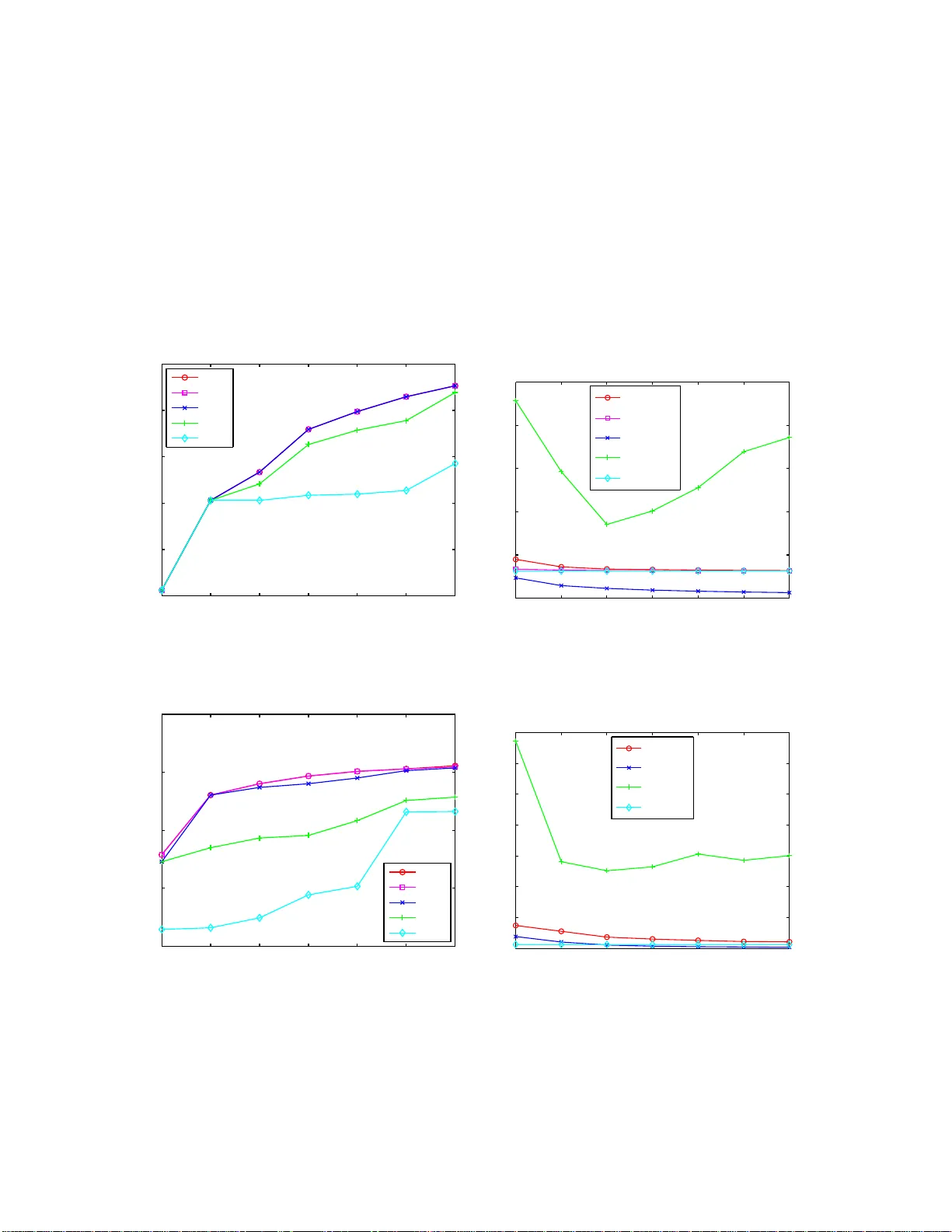
Submodul ar meets Spectra l: Greedy Algor ithms for Subset Selection, Sparse Approxim ation and Dictionary Selection Abhimanyu Das Univ ersity of Southern C alifornia abhimand@u sc.edu Da vid Ke mpe ∗ Univ ersity of Southern California c l kempe @ usc.edu Abstract W e study the prob lem of s electing a subset of k random variables from a large set, in order to obtain the b est linear prediction of ano ther variable o f interest. This p roblem can b e v iewed in the con text o f both feature selection and spar se approx imation. W e analyze the perfor mance of widely used greedy heuristics, using insights fro m the maximization of subm odular f unctions and spectral analy sis. W e introdu ce the submodu larity ratio as a key qua ntity to help u nderstand why gre edy algo rithms perfo rm well e ven when the variables are highly correlated. Using our tech niques, we obtain the stro ngest kno wn approx imation gu arantees for this problem, b oth in terms o f the submo dularity r atio and the smallest k -sparse eigenv alue of the cov ariance matrix. W e fu rther demo nstrate the wide ap plicability of o ur techn iques by an alyzing greedy algo rithms for the diction ary selection problem, and significantly impr ove the previously known guarantees. Ou r theo- retical analysis is comp lemented by experim ents on real-world an d syn thetic data sets; the exper iments show th at th e sub modula rity ratio is a stro nger pred ictor of the perform ance of gre edy algorith ms than other spectral param eters. 1 Introd uction W e analyze algorithms for the follo wing important Subset Selection probl em: select a subset of k v ari ables from a gi ven s et of n obs erv atio n va riables which , tak en tog ether , “best” predic t anothe r vari able of in terest . This pr oblem has many application s ranging from feature selec tion, sparse le arning and dictionar y selection in machine learni ng, to sp arse approximatio n and compress ed sens ing in signal proce ssing. From a machine learnin g persp ecti v e, the variab les co uld b e feature s or observ able attribu tes of a phenomen on, and we wish to predi ct the phenomenon using only a small subset from the high-dimen sional feature spac e. In signal proces sing, the variab les could correspond to a colle ction of dictionary ve ctors, and the goal is to parsimon iously represen t another (outp ut) vector . For many practition ers, the predictio n model of choice is linear regress ion, and the goal is to obtain a linear model using a small subset of var iables, to minimize the mean square predict ion error or , equi valen tly , maximize the squa red m ultiple correla tion R 2 [6]. Thus, we formula te the Subset Selection problem for regr ession as follo ws: Giv en the (normaliz ed) cov ariance s between n v ariable s X i (which can in princip le be observed ) and a variab le Z (which is to be predic ted), select a subse t of k ≪ n of the vari ables X i and a linear prediction functio n of Z from the selecte d X i that maximizes the R 2 fit. (A formal definition is giv en in Section 2 .) The cov ariances are usuall y obtained empirically from detai led past obser v ations of the v ariable values . ∗ Supported in part by NSF CAREER award 054 5855, and NSF grant dddas-tmrp 0540420 1 The abo ve formulation is known [2 ] to be equi val ent to the problem of sparse appr oximation ov er dictio nary vector s: t he input consists of a dictionar y of n featu re vector s x i ∈ R m , along with a targ et vec tor z ∈ R m , and the goal is to select at most k vectors w hose linear combinat ion best approximates z . The pairwise cov ariances of the pre vious formulation are then e xactly the inner prod ucts of the dicti onary vec tors. 1 Our prob lem formulation appe ars somewhat similar to the prob lem of sparse recove ry [17, 18, 19, 1]; ho weve r , note that in spars e reco very , it is generally assumed that the predict ion vecto r is truly (almost) k -sparse, and the aim is to recov er the exac t coef ficients of this truly spars e soluti on. Ho wev er , finding a sparse s olutio n is a well-moti vated pro blem e ven if the true solu tion is not spars e. E ven then, r unning sub set selecti on to find a sparse approx imation to the correc t soluti on helps to reduce cost and model comple xity . This proble m is NP -hard [11 ], so no polynomial- time algorith ms are kno wn to solv e it optimally for all input s. T wo appro aches are freque ntly used for approxi mating such problems: greedy algorit hms [10, 14, 5, 17] and con vex relaxation schemes [13, 1, 15, 4 ]. For our formulation, a disadv antage of con ve x relaxa tion techniq ues is that they do not provide e xplicit control ov er the targ et sparsity lev el k o f the soluti on; additi onal effort is neede d to tune the reg ulariza tion parameter . A simp ler and more intuiti ve appro ach, widely use d in practice for su bset selection proble ms (for e xam- ple, it is implemen ted in all commercial statistics pac kages) , is to use greedy algo rithms, which iter ati vely add or remove v ariabl es based on simple measures of fi t with Z . T wo of the most well-kno wn and w idely used greedy algorithms are the subject of our analysis: Forward Regressio n [10] and O rthogo nal Matching Pursuit [14]. (These algori thms are defined formally in Section 2). So far , the theore tical bounds on such greedy algorith ms hav e been unable to expla in why the y perform well in practice for most subset select ion problem instances. Most prev ious results for greedy subset se- lection algorithms [5, 14, 2] hav e been based on coherence of the input data, i.e., the maximum correlat ion µ between any pair of v ariables. Small coher ence is an ex tremely strong conditio n, and the bounds usu- ally break down when the coherence is ω (1 /k ) . On the other hand, most bounds for greedy and con ve x relaxa tion algori thms for sparse recov ery are based on a weaker sparse -eigen valu e or R estricte d Isometry Property (RIP) condi tion [18, 17, 9, 20, 1]. Howe ver , these results apply to a diffe rent objecti ve: minimiz- ing the differe nce betwee n the actual and estimated coef ficients of a sparse v ector . Simply extending these results to the subset selectio n prob lem adds a depen dence on the large st k -sparse eigen v alue and only leads to weak a dditi ve bound s. More importantly , all the abo ve res ults rely on s pectra l condition s that suf fer from an inabilit y to exp lain the performance of the algorithms for near -singular matrices. Eigen v alue-based bounds fail to explai n an observ ation of m any e xperimen ts (includ ing ours in Section 5): greed y algorit hms often per form ver y well, eve n for near -singular input matric es. Our results be gin to exp lain thes e observ ations by proving that the perfo rmance of many algo rithms does not really depend on ho w singular the co varia nce matrix is, b ut rather on ho w far the R 2 measure de viates from submod ularity on the giv en input. W e formalize this intuition by defining a measure of “approximate submod ularity ” which we term submodu larity ratio . W e pro ve that whenev er the submodu larity ratio is boun ded awa y fro m 0, the R 2 object i ve is “reaso nably close ” to submodu lar , and Forward Regress ion gi ves a constant- fact or approx imation. This significa ntly generaliz es a recent result of Das and Kempe [2], who had identified a strong condition termed “absence o f con dition al suppress ors” which ensure s tha t the R 2 object i ve is a ctually submodu lar . An analys is based on the submodularity ratio does relate w ith traditional spect ral bounds, in that the ratio is al ways lower -bounded by th e smallest k -sparse eig en v alue of C (though it can b e sign ifi cantly lar ger 1 For this reason, the dimension m of the feature ve ctors o nly af fects the problem indirectly , via the accuracy of the estimated cov ariance matrix. 2 when the pr edicto r v ariable is not badl y aligned with the ei genspa ce of small eig en v alues). In partic ular , we also ob tain multiplic ati ve approximation guaran tees for both Fo rward Regressio n and Orthogo nal Matching Pursuit, whene ver the smallest k -sparse eigen v alue of C is bounded away from 0 , significantly strengthen ing past kno wn bound s on their performance. An adde d benefit of our frame work is that we obt ain much tigh ter theoretical performan ce guarantees for gree dy algorithms for diction ary selection [8 ]. In the di ctiona ry selecti on pr oblem , we are giv en s target vec tors, and a candidat e set V of feature vecto rs. The goal is to select a set D ⊂ V of at m ost d feature vec tors, which will serv e as a dictionary in the follo wing sense. For each of sev eral targ et vectors , the best k < d vecto rs from D will be selected and used to achie ve a good R 2 fit; the goal is to maximize the a ver age R 2 fit for all of these vec tors. (A formal definition is giv en in Section 2.) This probl em of finding a dictio nary of basis functio ns for sparse representati on of signals has s eve ral application s in mach ine learning and signal proce ssing. Krause and Ce vher [8] showed that gre edy algorithms for dictiona ry selectio n can perfor m w ell in many instances, and prove d additi ve approximati on boun ds for two specific algorithms , SDS MA and SDS OMP (defined in Section 4). Our approximate submodula rity framew ork allo ws us to obtain much stronge r m ultipli cati ve guarantees without much extra ef fort. Our theoretica l analys is is complemented by experimen ts comparing the performan ce of the greedy algori thms and a baseline con vex-re laxatio n algorithm for su bset selection on tw o real-wor ld data sets and a synthe tic data set. More importantly , we ev aluate the submodular ity ratio of these data sets and compare it with other spectral parameters: while the input cov ariance matrices are close to singular , the submodul arity ratio actually turn s out to be sig nificantly lar ger . Thus, our theore tical result s can begin to explain why , in many instances, greed y algori thms perform well in spit e of the fac t that the data ma y h ave h igh c orrela tions. Our main contrib utions can be summarized as follo ws: 1. W e introduce the notio n of the submodula rity ratio as a much more accurate predic tor of the perfo r - mance of greedy algorith ms than pre viously used paramet ers. 2. W e obtain the stro ngest kno wn theoretical performance guarantee s for greedy algor ithms for subset selecti on. In particular , we show (in Section 3) that the Forward Reg ression and O MP algorit hms are within a 1 − e − γ fact or and 1 − e − ( γ · λ min ) fact or of the optimal solution, respecti vely (where the γ and λ terms are appro priate submodu larity and sparse -eigen valu e parameter s). 3. W e obtai n the strong est known th eoretical guaran tees for algori thms for dictiona ry selectio n, improv- ing on the results of [8]. In particu lar , we sho w (in Section 4) that the SDS MA algori thm is within a fact or γ λ max (1 − 1 e ) of optimal . 4. W e ev aluate our theoretical boun ds for subset selectio n by runnin g greedy and L1-relaxation algo- rithms on real-world and synth etic data, and sho w ho w the vari ous submodula r and spectral parame- ters correla te with the perfor mance of the algorith ms in practice . 1.1 Related W ork As mentioned pre viously , there has been a lot of recent interest in greedy and con ve x rela xation techniques for the sparse reco very problems, both in the noiseless and nois y settin g. For L1 relaxa tion techniques, Tropp [15] sho wed condition s based on the cohere nce (i.e., the maximum correla tion between any pair of variab les) of the dictiona ry that guarantee d near- optimal reco ver y of a sparse signal. In [1, 4], it was sho wn that if the tar get signal is truly sparse, an d the diction ary obeys a restr icted iso m etry pro perty (RIP), then L1 re laxati on can almost exac tly recov er the true spa rse signal. Other results [19, 20] also pro ve conditi ons unde r which 3 L1 relax ation can recov er a sparse signal. T hough relate d, the abo ve results are not directly applicab le to our subset sele ction formulat ion, since the goal in sparse recov ery is to recov er the true coef ficients of the sparse signal , as oppos ed to our problem of minimizing the predictio n erro r of an arbitrary signal subjec t to a specified sparsi ty le vel . For greedy sparse reco very , Zhang [17, 18] and Lozano et al. [9] pro vided conditions based on spa rse eigen value s under which Forward Regressi on and Forward-Back ward Regre ssion can recov er a sparse sig- nal. As with the L1 results for sparse recove ry , the objecti ve functio n analyze d in these papers is some what dif ferent from that in our s ubset selection formula tion; furthermore, these results ar e inte nded mainly fo r the case when the predictor v ariable is truly sparse. Simply exten ding these results to our problem formulation gi ves weaker , additi ve bounds and require s stronger condi tions than our results . The papers by Das and K empe [2], Gil bert e t al. [5] and Trop p et al. [1 6, 1 4 ] an alyzed g reedy algo rithms using the same s ubset selectio n formula tion p resented in this work. In particular , they obtain ed a 1 + Θ( µ 2 k ) multiplic ati ve appr oximatio n guaran tee for the mean square error objecti ve and a 1 − Θ( µk ) guarantee for the R 2 object i ve, whene ver the coheren ce µ of the dicti onary is O (1 /k ) . T hese result s are thus weaker tha n those present ed here, since the y do not apply to instances with ev en moderate correlation s of ω (1 /k ) . Other analysis of greedy methods in cludes the work of Natarajan [11], which pr ov ed a bicriteria a pprox- imation bound for minimizin g the number of vec tors needed to achie ve a giv en prediction error . As men tioned earl ier , the paper by Krause and C e vher [8] analyzed gree dy algorith ms for the dictionary selecti on problem, which generali zes subs et selectio n to prediction of multiple var iables . They too use a notion of appro ximate submodularity to provi de addit i ve approximatio n guarantees. S ince their analysis is for a more gener al problem than subse t selection , applying their results directly to the subset selection proble m predictab ly gi ves much weak er bound s than those presented in this paper for subset selecti on. Furthermor e, eve n for the general dictionar y sele ction problem, our techniq ues can be used to significan tly impro ve their analysis of greedy algorit hms and obta in tighter multiplicati ve approximat ion bounds (as sho wn in Section 4). In gener al, we note that the performa nce boun ds for greedy algorithms deri ved using the coherenc e paramete r are usual ly the w eake st, followed by those using the Restricted Isometry Property , then those using spar se eigen v alues, and fi nally those using the submodularit y ratio. (W e sho w an empirical compariso n of these paramete rs in Section 5.) 2 Pr eliminaries The goal in subse t selec tion is to estimate a pr edictor variable Z using linear re gression on a small subse t from the set of observa tion variables V = { X 1 , . . . , X n } . W e use V a r( X i ) , Co v ( X i , X j ) and ρ ( X i , X j ) to denote the vari ance, cov arianc e and correl ation of rando m varia bles, respe cti vely . By approp riate nor - malizatio n, we can assume that all the random v ariables ha ve expectat ion 0 and v ariance 1. T he matrix of cov ariance s between the X i and X j is den oted by C , with ent ries c i,j = Co v ( X i , X j ) . Similarly , we use b to denote the cov ariance s between Z and the X i , with entries b i = C o v ( Z, X i ) . Formal ly , the Subset Select ion proble m can no w be state d as follo ws: Definition 2.1 (Subset Selection) Given pair wise covar iances among all vari ables, as well as a par ameter k , find a set S ⊂ V of at most k variables X i and a linea r pr edictor Z ′ = P i ∈ S α i X i of Z , maximizin g the square d multiple correlation [3, 6] R 2 Z,S = V ar( Z ) − E  ( Z − Z ′ ) 2  V ar( Z ) . 4 R 2 is a widely used m easure for the goodness of a statistical fit; it captures the fraction of the var iance of Z expla ined by var iables in S . B ecause we assumed Z to be normaliz ed to hav e varia nce 1, it simplifies to R 2 Z,S = 1 − E  ( Z − Z ′ ) 2  . For a set S , we use C S to denote the submatrix of C with row and column set S , and b S to denote the vec tor with only entries b i for i ∈ S . For notation al con v enienc e, w e frequentl y do not distingu ish between the index set S and the varia bles { X i | i ∈ S } . Giv en the subset S of va riables used for prediction , the optimal re gression coef ficients α i are well kno wn to be a S = ( α i ) i ∈ S = C − 1 S · b S (see, e .g., [6]), a nd henc e R 2 Z,S = b T S C − 1 S b S . Thus, the sub set selectio n problem c an b e p hrased as follows: Giv en C , b , a nd k , se lect a set S of at most k v ariable s to maximize R 2 Z,S = b T S ( C − 1 S ) b S . 2 The dictio nary selection problem gener alizes the subset selection proble m by consider ing s predic tor v ariables Z 1 , Z 2 , . . . , Z s . The goal is to select a dictionar y D of d observ ation varia bles, to optimize the a ver age R 2 fit for the Z i using at most k vectors from D for each. Formally , the Dictionary Selection proble m is defined as follo ws: Definition 2.2 (Dictionary Selection) Given all pairwise covar iances among the Z j and X i variab les, as well as par ameter s d and k , find a set D of at m ost d vari ables fr om { X 1 , . . . , X n } maximizing F ( D ) = s X j =1 max S ⊂ D , | S | = k R 2 Z j ,S . Many of ou r results are phrased in terms of eigen valu es of the cov arianc e matrix C and its submatrices. Since cov ariance matrices are positi ve semidefinite, their eigen value s are real and non-neg ativ e [6]. For any positi ve semide finite n × n matrix A , we denote its eigen v alues by λ min ( A ) = λ 1 ( A ) ≤ λ 2 ( A ) ≤ . . . ≤ λ n ( A ) = λ max ( A ) . W e use λ min ( C, k ) = min S : | S | = k λ min ( C S ) to refer to the smallest eigen- v alue of any k × k submat rix of C (i.e., the smallest k -sparse eigen va lue), and similarl y λ max ( C, k ) = max S : | S | = k λ max ( C S ) . 3 W e also use κ ( C, k ) to deno te the lar gest conditi on number (the ratio of the large st and smallest eigen v alue) of any k × k submatrix of C . This quanti ty is strongl y r elated to the Restricted Isom- etry Prope rty in [1]. W e also use µ ( C ) = max i 6 = j | c i,j | to de note the coher ence , i.e., the maximum abs olute pairwise correla tion between the X i v ariables. Recall the L 2 vec tor and matrix norms: k x k 2 = p P i | x i | 2 , and k A k 2 = λ max ( A ) = max k x k 2 =1 k A x k 2 . W e also use k x k 0 = |{ i | x i 6 = 0 }| to denote the sparsity of a vec tor x . The part of a varia ble Z that is not correlat ed with the X i for all i ∈ S , i.e., the part that cannot be exp lained by the X i , is called the r esidual (see [3]), and defined as Res( Z, S ) = Z − P i ∈ S α i X i . 2.1 Submodularity Ratio W e introduc e the notion of submodular ity ratio for a general set function , which captures “how close” to submodu lar the fu nction is. W e first define it for a rbitrary set fun ctions , and then sh ow the specializat ion for the R 2 object i ve. Definition 2.3 (Submodularity Ratio) Let f be a non-ne gativ e set functi on. The submodul arity rati o of f with r espect to a set U and a paramet er k ≥ 1 is γ U,k ( f ) = min L ⊆ U,S : | S |≤ k ,S ∩ L = ∅ P x ∈ S f ( L ∪ { x } ) − f ( L ) f ( L ∪ S ) − f ( L ) . 2 W e assume throughout that C S is non-singu lar . For some of our results, an e xtension to singular matrices is possible using the Moore-Penrose generalized in verse. 3 Computing λ min ( C, k ) is NP-hard. In Appendix A we describe ho w to efficiently approximate the valu es for some scenarios. 5 Thus, it captu r es how much mor e f can incr ease by adding any subset S of size k to L , compar ed to the combined benefi ts of addin g its indivi dual elements to L . If f is specifically the R 2 object ive define d on the variab les X i , then we omit f and simply define γ U,k = min L ⊆ U,S : | S |≤ k ,S ∩ L = ∅ P i ∈ S ( R 2 Z,L ∪{ X i } − R 2 Z,L ) R 2 Z,S ∪ L − R 2 Z,L = min L ⊆ U,S : | S |≤ k ,S ∩ L = ∅ ( b L S ) T b L S ( b L S ) T ( C L S ) − 1 b L S , wher e C L and b L ar e the normalized covarian ce matrix and normalized covar iance vecto r corr esponding to the set { Res( X 1 , L ) , Res( X 2 , L ) , . . . , Res ( X n , L ) } . It can be easily sho w n that f is submodu lar if and only if γ U,k ≥ 1 , for all U and k . For the purpose of subset selecti on, it is significant that the submodu larity ratio can be bounde d in terms of the smallest sparse eigen value , as sho wn in the follo wing lemma: Lemma 2.4 γ U,k ≥ λ min ( C, k + | U | ) ≥ λ min ( C ) . For all o ur analysis in this pa per , we will use | U | = k , and henc e γ U,k ≥ λ min ( C, 2 k ) . T hus, the smallest 2 k -sparse eig en v alue is a lower bound on this submod ularity ratio; as w e s ho w later , it is often a weak lo wer bound . Before provi ng Lemma 2.4, we first introduce two lemmas that relate the eigen val ues of normalize d cov ariance matrices with those of its submatrices. Lemma 2.5 Let C be the cova riance m atrix of n zer o-mean rando m variab les X 1 , X 2 , . . . , X n , eac h of which has variance at most 1 . Let C ρ be the corr esponding corr elation matrix of the n r andom variables, that is, C ρ is the co variance matrix of the variab les after the y ar e normal ized to have unit varian ce. Then λ min ( C ) ≤ λ min ( C ρ ) . Pro of. Since C ρ is obtained by normaliz ing the vari ables suc h that they ha ve unit v ariance, we get C ρ = D T C D , where D is a diagon al matrix with diagonal entries d i = 1 √ V ar( X i ) . Since both C ρ and C are positi ve semidefinit e, we can perform Cholesky factori zation to get lower - triang ular m atrices A ρ and A such that C = AA T and C ρ = A ρ A T ρ . Hence A ρ = D T A . Let σ min ( A ) and σ min ( A ρ ) den ote the smalles t singular v alues of A an d A ρ , respe cti vely . Also, let v be the singul ar vector correspo nding to σ min ( A ρ ) . Then, k A v k 2 = k D − 1 A ρ v k 2 ≤ k D − 1 k 2 k A ρ v k 2 = σ min ( A ρ ) k D − 1 k 2 ≤ σ min ( A ρ ) , where the last inequal ity follo ws since k D − 1 k 2 = max i 1 d i = max i p V ar( X i ) ≤ 1 . Hence, by the Courant- Fischer theorem, σ min ( A ) ≤ σ min ( A ρ ) , and consequen tly , λ min ( C ) ≤ λ min ( C ρ ) . Lemma 2.6 Let λ min ( C ) be the smallest eigen valu e of the covarian ce matrix C of n ran dom variables X 1 , X 2 , . . . , X n , and λ min ( C ′ ) be the smallest eigen valu e of the ( n − 1) × ( n − 1) covari ance matrix C ′ corr espon ding to the n − 1 random variab les Res( X 1 , X n ) , . . . , Res( X n − 1 , X n ) . Then λ min ( C ) ≤ λ min ( C ′ ) . 6 Pro of. Let λ i and λ ′ i denote the eigen value s of C and C ′ respec ti vely . Also, let c ′ i,j denote the entries of C ′ . Using the definit ion of the resid ual, we get that c ′ i,j = Co v (Res( X i , X n ) , Res ( X j , X n )) = c i,j − c i,n c j,n c n,n , c ′ i,i = V ar(Res( X i , X n )) = c i,i − c 2 i,n c n,n . Defining D = 1 c n,n · [ c 1 ,n , c 2 ,n , . . . , c n − 1 ,n ] T · [ c 1 ,n , c 2 ,n , . . . , c n − 1 ,n ] , we can write C { 1 ,...,n − 1 } = C ′ + D . T o pro ve λ 1 ≤ λ ′ 1 , let e ′ = [ e ′ 1 , . . . , e ′ n − 1 ] T be the eigen vect or of C ′ corres pondin g to the eigen valu e λ ′ 1 , and consid er the vect or e = [ e ′ 1 , e ′ 2 , . . . , e ′ n − 1 , − 1 c n,n P n − 1 i =1 e ′ i c i,n ] T . Then, C · e = [ y 0 ] , where y = − 1 c n,n n − 1 X i =1 e ′ i c i,n [ c 1 ,n , c 2 ,n , . . . , c n − 1 ,n ] T + C { 1 ,...,n − 1 } · e ′ = − 1 c n,n n − 1 X i =1 e ′ i c i,n [ c 1 ,n , c 2 ,n , . . . , c n − 1 ,n ] T + D · e ′ + C ′ · e ′ = C ′ · e ′ . Thus, C · e = [ λ ′ 1 e ′ 1 , λ ′ 1 e ′ 2 , . . . , λ ′ 1 e ′ n − 1 , 0] T = λ ′ 1 [ e ′ 1 , e ′ 2 , . . . , e ′ n − 1 , 0] T ≤ λ ′ 1 k e k 2 , which by Rayleigh- Ritz boun ds implies that λ 1 ≤ λ ′ 1 . Using the abov e two lemmas, we now pr ov e Lemma 2.4. Pro of of Lemma 2.4. Since ( b L S ) T ( C L S ) − 1 b L S ( b L S ) T b L S ≤ max x x T ( C L S ) − 1 x x T x = λ max (( C L S ) − 1 ) = 1 λ min ( C L S ) , we can use Definition 2.3 to obtain that γ U,k ≥ m in ( L ⊆ U,S : | S |≤ k ,S ∩ L = ∅ ) λ min ( C L S ) . Next, we relate λ min ( C L S ) with λ min ( C L ∪ S ) , using repeate d applic ations of Lemmas 2.5 and 2.6 . Let L = { X 1 , . . . , X ℓ } ; for each i , define L i = { X 1 , . . . , X i } , and let C ( i ) be the cov arianc e matrix of the random varia bles { Res( X , L \ L i ) | X ∈ S ∪ L i } , and C ( i ) ρ the cov ariance m atrix after normaliz ing all its v ariables to unit vari ance. T hen, L emma 2.5 implies that for each i , λ min ( C ( i ) ) ≤ λ min ( C ( i ) ρ ) , and Lemma 2.6 shows that λ min ( C ( i ) ρ ) ≤ λ min ( C ( i − 1) ) for each i > 0 . Combining these inequa lities inducti vely for all i , we obtai n that λ min ( C L S ) = λ min ( C (0) ρ ) ≥ λ min ( C ( ℓ ) ) = λ min ( C L ∪ S ) ≥ λ min ( C, | L ∪ S | ) . Finally , since | S | ≤ k and L ⊆ U , we obta in γ U,k ≥ λ min ( C, k + | U | ) . 3 Algorithms Analysis W e no w present theoretical performance bounds for Forward Re gression and Orthogonal Matching Pursuit, which are widely used in practice. W e also analyze the Oblivio us algorith m: one of the simplest greedy algori thms for subset select ion. Thro ughou t this section, we use OPT = max S : | S | = k R 2 Z,S to denote the optimum R 2 v alue achiev able by any set o f size k . 7 3.1 Forward Regr ession W e fi rst provid e approx imation boun ds for Forward Regression , which is the standard algorith m used by many re search ers in medical, social, and economic domains. 4 Definition 3.1 (Fo rward Regr ession) The Forward Regressi on (al so cal led Forw ard Selection ) algorithm for subset selecti on selects a set S of size k iter atively as follows: 1: Initialize S 0 = ∅ . 2: for eac h iter ation i + 1 do 3: Let X m be a variab le m aximizing R 2 Z,S i ∪{ X m } , and set S i +1 = S i ∪ { X m } . 4: Output S k . Our main result is the follo wing theorem. Theor em 3.2 T he set S FR selecte d by forwar d re gr ession has the following appr oximation guaran tees: R 2 Z,S FR ≥ (1 − e − γ S FR ,k ) · OPT ≥ (1 − e − λ min ( C, 2 k ) ) · OPT ≥ (1 − e − λ min ( C,k ) ) · Θ(( 1 2 ) 1 /λ min ( C,k ) ) · OPT . Before provi ng the theorem, we first begin with a gene ral lemma that bound s the amount by which the R 2 v alue of a set and the sum of R 2 v alues of its elements can dif fer . Lemma 3.3 1 λ max ( C ) P n i =1 R 2 Z,X i ≤ R 2 Z, { X 1 ,...,X n } ≤ 1 γ ∅ ,n P n i =1 R 2 Z,X i ≤ 1 λ min ( C ) P n i =1 R 2 Z,X i . Pro of. Let the eigen valu es of C − 1 be λ ′ 1 ≤ λ ′ 2 ≤ . . . ≤ λ ′ n , with corres pondi ng orthon ormal eigen vector s e 1 , e 2 , . . . , e n . W e write b in the basis { e 1 , e 2 , . . . , e n } as b = P i β i e i . Then, R 2 Z, { X 1 ,...,X n } = b T C − 1 b = X i β 2 i λ ′ i . Because λ ′ 1 ≤ λ ′ i for all i , we get λ ′ 1 P i β 2 i ≤ R 2 Z, { X 1 ,...,X n } , and P i β 2 i = b T b = P i R 2 Z,X i , because the length of the vector b is independ ent of the basis it is written in. Also, by definit ion of the submodu larity ratio, R 2 Z, { X 1 ,...,X n } ≤ P i β 2 i γ ∅ ,n . Finally , becau se λ ′ 1 = 1 λ max ( C ) , and using Lemma 2.4, we obtain the result. The ne xt lemma r elates the optimal R 2 v alue using k elements to the opti mal R 2 using k ′ < k elements. Lemma 3.4 F or ea ch k , let S ∗ k ∈ argmax | S |≤ k R 2 Z,S be an optimal subset of at most k variables. T hen, for any k ′ = Θ( k ) suc h that 1 λ min ( C,k ) < k ′ < k , we have that R 2 Z,S ∗ k ′ ≥ R 2 Z,S ∗ k · Θ(( k ′ k ) 1 /λ min ( C,k ) ) , for lar ge enoug h k . In particula r , R 2 Z,S ∗ k/ 2 ≥ R 2 Z,S ∗ k · Θ(( 1 2 ) 1 /λ min ( C,k ) ) , for lar ge enough k . 4 There i s some inconsistency i n the literature about naming of greedy algorithms. Forw ard Regression is sometimes also referred to as Orthogonal Matching Pursuit (OMP). W e choose the nomenclature consistent with [10] and [14]. 8 Pro of. W e first prov e that R 2 Z,S ∗ k − 1 ≥ (1 − 1 k λ min ( C,k ) ) R 2 Z,S ∗ k . Let T = Res( Z , S ∗ k ) ; then, Co v ( X i , T ) = 0 for all X i ∈ S ∗ k , and Z = T + P X i ∈ S ∗ k α i X i , w here α = ( α i ) = C − 1 S ∗ k · b S ∗ k are the optimal regres sion coef ficients. W e write Z ′ = Z − T . For an y X j ∈ S ∗ k , by definitio n of R 2 , we ha ve that R 2 Z ′ ,S ∗ k \{ X j } = 1 − α 2 j V ar( X j ) V ar( Z ′ ) = 1 − α 2 j V ar( Z ′ ) ; in parti cular , this implies that R 2 Z ′ ,S ∗ k − 1 ≥ 1 − α 2 j V ar( Z ′ ) for all X j ∈ S ∗ k . Focus now on j m inimizing α 2 j , so that α 2 j ≤ k α k 2 2 k . As in the p roof of Lemma 3.3 , by writing α in terms of an orthonorma l eigenbasi s of C S ∗ k , one can sho w that | α T C S ∗ k α | ≥ k α k 2 2 λ min ( C S ∗ k ) , or k α k 2 2 ≤ | α T C S ∗ k α | λ min ( C S ∗ k ) . Furthermor e, α T C S ∗ k α = V ar( P X i ∈ S ∗ k α i X i ) = V ar( Z ′ ) , so R 2 Z ′ ,S ∗ k − 1 ≥ 1 − 1 k λ min ( C S ∗ k ) . F inally , by definitio n, R 2 Z ′ ,S ∗ k = 1 , so R 2 Z,S ∗ k − 1 R 2 Z,S ∗ k ≥ R 2 Z ′ ,S ∗ k − 1 R 2 Z ′ ,S ∗ k ≥ 1 − 1 k λ min ( C S ∗ k ) ≥ 1 − 1 k λ min ( C, k ) . No w , applying this inequality repeatedl y , we get R 2 Z,S ∗ k ′ ≥ R 2 Z,S ∗ k · k Y i = k ′ +1 (1 − 1 iλ min ( C, i ) ) . Let t = ⌈ 1 /λ min ( C, k ) ⌉ , so tha t the pre vious bound implies R 2 Z,S ∗ k ′ ≥ R 2 Z,S ∗ k · Q k i = k ′ +1 i − t i . Most o f the terms in the product telescop e, givin g us a bound of R 2 Z,S ∗ k · Q t i =1 k ′ − t + i k − t + i . Since Q t i =1 k ′ − t + i k − t + i con v er ges to ( k ′ k ) t with incre asing k (keep ing t constant), w e get that for lar ge k , R 2 Z,S ∗ k ′ ≥ R 2 Z,S ∗ k · Θ(( k ′ k ) t ) ≥ R 2 Z,S ∗ k · Θ(( k ′ k ) 1 /λ min ( C,k ) ) . Using the abov e lemmas, we now pro ve the main theorem. Pro of of Theorem 3.2. W e begin by pro ving the fi rst inequality . Let S ∗ k be the optimum set of v ariables. Let S G i be the set of varia bles chosen by Forward Reg ression in the first i iterations, and S i = S ∗ k \ S G i . By monoton icity of R 2 and the fact that S i ∪ S G i ⊇ S ∗ k , we ha ve that R 2 Z,S i ∪ S G i ≥ OPT. For each X j ∈ S i , let X ′ j = Res( X j , S G i ) be the residual of X j condit ioned on S G i , and write S ′ i = { X ′ j | X j ∈ S } . W e will sho w that at least one of the X ′ i is a good cand idate in iteration i + 1 of Forward R egre ssion. First, the joint contrib ution of S ′ i must be fairly lar ge: R 2 Z, Res( S ′ i ,S G i ) = R 2 Z,S ′ i ≥ OPT − R 2 Z,S G i . U sing Definition 2.3, as well as S G i ⊆ S FR and | S i | ≤ k , X X ′ j ∈ S ′ i R 2 Z,X ′ j ≥ γ S G i , | S i | · R 2 Z,S ′ i ≥ γ S FR ,k · R 2 Z,S ′ i . 9 Let ℓ maximize R 2 Z,X ′ ℓ , i.e., ℓ ∈ argmax ( j : X ′ j ∈ S ′ i ) R 2 Z,X ′ j . Then we get that R 2 Z,X ′ ℓ ≥ γ S FR ,k | S ′ i | · R 2 Z,S ′ i ≥ γ S FR ,k k · R 2 Z,S ′ i . Define A ( i ) = R 2 Z,S G i − R 2 Z,S i − 1 G to be the gain obtained fr om the varia ble chosen by Forward Regression in iteration i . Then R 2 Z,S FR = P k i =1 A ( i ) . Since the X ′ ℓ abo ve was a ca ndida te to be chosen in iteratio n i + 1 , and Forwa rd Regr ession chose a v ariable X m such that R 2 Z, Res( X m ,S G i ) ≥ R 2 Z, Res( X,S G i ) for all X / ∈ S G i , we obtain that A ( i + 1) ≥ γ S FR ,k k · R 2 Z,S ′ i ≥ γ S FR ,k k ( OPT − R 2 Z,S G i ) ≥ γ S FR ,k k ( OPT − i X j =1 A ( j )) . Since the abo ve inequalit y hold s for each iterati on i = 1 , 2 , . . . , k , a simple induc ti ve proof establishe s the bound OPT − P k i =1 A ( i ) ≤ OPT · (1 − γ S FR ,k k ) k . Hence, R 2 Z,S FR = k X i =1 A ( i ) ≥ OPT − OP T (1 − γ S FR ,k k ) k ≥ OPT · (1 − e − γ S FR ,k ) . The second inequ ality follo ws direc tly from L emma 2.4, and the fact tha t | S FR | = k . By applying the abo ve result after k / 2 iterations, we obtain R 2 Z,S G k/ 2 ≥ (1 − e − λ min ( C,k ) ) · R 2 Z,S ∗ k/ 2 . No w , using Lemma 3.4 and monoton icity of R 2 , we get R 2 Z,S G k ≥ R 2 Z,S G k/ 2 ≥ (1 − e − λ min ( C,k ) ) · Θ(( 1 2 ) 1 /λ min ( C,k ) ) · R 2 Z,S ∗ k , pro ving the third inequal ity . 3.2 Orthogonal Matching Pursuit The second greedy algorit hm w e analyz e is Orthogo nal Matching P ursuit (OMP), freque ntly used in signal proces sing domains. Definition 3.5 (Orthogonal Matching Pursuit (OMP)) The Orthogon al Matching Pursuit algor ithm for subset selecti on selects a set S of size k iter atively as follows: 1: Initialize S 0 = ∅ . 2: for eac h iter ation i + 1 do 3: Let X m be a variab le m aximizing | Co v (Res( Z , S i ) , X m ) | , and set S i +1 = S i ∪ { X m } . 4: Output S k . By applyi ng similar techni ques as in the pre vious section, we can also obtain approximatio n bounds for OMP . W e start by pro ving the follo wing lemma that lower -bounds the v ariance of the resid ual of a var iable. Lemma 3.6 Let A be the ( n + 1) × ( n + 1) covarian ce matrix of the normal ized varia bles Z, X 1 , X 2 , . . . , X n . Then V ar(Res( Z, { X 1 , . . . , X n } )) ≥ λ min ( A ) . 10 Pro of. The matrix A is of the form A =  1 b T b C  . W e use A [ i, j ] to denote the matrix obtained by remov ing the i th ro w and j th column of A , and similarly for C . Recalling that the ( i, j ) entry of C − 1 is ( − 1) i + j det( C [ i,j ]) det( C ) , and de vel oping the determinan t of A by the first ro w and column, we can w rite det( A ) = n +1 X j =1 ( − 1) 1+ j a 1 ,j det( A [1 , j ]) = det( C ) + n X j =1 ( − 1) j b j det( A [1 , j + 1]) = det ( C ) + n X j =1 ( − 1) j b j n X i =1 ( − 1) i +1 b i det( C [ i, j ]) = det( C ) − n X j =1 n X i =1 ( − 1) i + j b i b j det( C [ i, j ]) = det( C )(1 − b T C − 1 b ) . Therefore , using that V ar( Z ) = 1 , V ar(Res( Z, { X 1 , . . . , X n } )) = V ar( Z ) − b T C − 1 b = det( A ) det( C ) . Because d et( A ) = Q n +1 i =1 λ A i and det( C ) = Q n i =1 λ C i , and λ A 1 ≤ λ C 1 ≤ λ A 2 ≤ λ C 2 ≤ . . . ≤ λ A n +1 by the eigen value interlacing theorem, w e get that det( A ) det( C ) ≥ λ A 1 , prov ing the lemma. The abov e lemma, along with an analysis similar to the proof of Theorem 3.2 , can be used to prove the follo wing appro ximation bound s for O MP: Theor em 3.7 T he set S OMP selecte d by orth ogo nal match ing pursui t has the following appr oximatio n guar - antees : R 2 Z,S OMP ≥ (1 − e − ( γ S OMP ,k · λ min ( C, 2 k )) ) · OPT ≥ (1 − e − λ min ( C, 2 k ) 2 ) · OPT ≥ (1 − e − λ min ( C,k ) 2 ) · Θ(( 1 2 ) 1 /λ min ( C,k ) ) · OPT . Pro of. W e be gin by proving the firs t ineq uality . U sing notation similar to th at in t he pr oof of Theo rem 3.2, we let S ∗ k be the optimum set of k variab les, S G i the set of variab les chosen by OMP in the first i iterations, and S i = S ∗ k \ S G i . Fo r each X j ∈ S i , let X ′ j = Res( X j , S G i ) be th e residual of X j condit ioned on S G i , and write S ′ i = { X ′ j | X j ∈ S } . Consider some iteration i + 1 of OMP . W e will show that at least one of the X ′ i is a good candidate in this iterati on. L et ℓ maximize R 2 Z,X ′ ℓ , i.e., ℓ ∈ argmax ( j : X ′ j ∈ S ′ i ) R 2 Z,X ′ j . By Lemma 3 . 7 , V ar ( X ′ ℓ ) ≥ λ min ( C S i G ∪{ X ′ ℓ } ) ≥ λ min ( C, 2 k ) . 11 The OM P algorithm chooses a var iable X m to add which maximiz es | Co v (Res( Z, S i G ) , X m ) | . Thus , X m maximizes Co v (Res( Z, S i G ) , X m ) 2 = Co v ( Z, Res( X m , S i G )) 2 = R 2 Z, Res( X m ,S i G ) · V ar(Res( X m , S i G )) . In parti cular , this implies R 2 Z, Res( X m ,S i G ) ≥ R 2 Z,X ′ ℓ · V ar ( X ′ ℓ ) V ar(Res ( X m , S i G )) ≥ R 2 Z,X ′ ℓ · λ min ( C, 2 k ) V ar(Res ( X m , S i G )) ≥ R 2 Z,X ′ ℓ · λ min ( C, 2 k ) , becaus e V ar(Res( X m , S i G )) ≤ 1 . As in the proof of Theorem 3.2, R 2 Z,X ′ ℓ ≥ γ S OMP ,k k · R 2 Z,S ′ i , so R 2 Z, Res( X m ,S i G ) ≥ R 2 Z,S ′ i · λ min ( C, 2 k ) · γ S OMP ,k k . W ith the same definiti on of A ( i ) as in the pre vious proof, we get t hat A ( i + 1) ≥ λ min ( C, 2 k ) γ S OMP ,k k ( P − P i j =1 A ( j )) . An inducti ve proof now sho ws that R 2 Z,S G = k X i =1 A ( i ) ≥ (1 − e − λ min ( C, 2 k ) · γ S OMP ,k ) · R 2 Z,S ∗ k . The proofs of the other two ine qualiti es follo w the same pattern as the proof for Forward Re gression. 3.3 Oblivious Algorithm As a baseline, w e also conside r a greedy algorithm which completely ignore s C and simply selects the k v ariables indi vidually most corre lated with Z . Definition 3.8 (Oblivio us) The Oblivi ous algori thm for subset selec tion is as follows: Select the k variables X i with the lar gest b i values . Lemma 3.3 immediately implies a simple bound for the Obli vious algorith m : Theor em 3.9 T he set S OBL selecte d by the Oblivious algo rithm has the follo wing appr oximati on guar an- tees: R 2 Z,S OBL ≥ γ ∅ ,k λ max ( C, k ) · OPT ≥ λ min ( C, k ) λ max ( C, k ) · OPT . Pro of. Let S be the set chosen by the Oblivio us algorithm, and S ∗ k the optimum set of k v ariable s. By definitio n of the Obli vious algorit hm, P i ∈ S R 2 Z,X i ≥ P i ∈ S ∗ k R 2 Z,X i , so using Lemma 3.3, we obtain that R 2 Z,S ≥ P i ∈ S R 2 Z,X i λ max ( C, k ) ≥ P i ∈ S ∗ k R 2 Z,X i λ max ( C, k ) ≥ γ ∅ ,k λ max ( C, k ) R 2 Z,S ∗ k . The secon d inequality of the theore m follo ws directl y from Lemma 2.4. 4 Dictionary Selection Bounds T o demonst rate the wider appl icabili ty of the approximate submodularity framew ork, we next obtain a tighte r analy sis for two gree dy algorithms for the dictionary selection problem, introduced in [8]. 12 4.1 The Algorithm SDS MA The SDS MA algori thm generaliz es the Obliv ious gre edy algorithm to the problem of dicti onary selectio n. It replac es the R 2 Z j ,S term in Definition 2.2 with its modular approximati on f ( Z j , S ) = P i ∈ S R 2 Z j ,X i . Thus, it greedily tries to m aximize the function ˆ F ( D ) = P s j =1 max S ⊂ D , | S | = k f ( Z j , S ) , ov er sets D of size at most d ; the inner maximum can be compute d efficientl y using the Obli vious algorithm. Definition 4.1 ( SDS MA ) The S DS MA algori thm for diction ary selecti on selects a dictionar y D of size d iter atively as follows: 1: Initialize D 0 = ∅ . 2: for eac h iter ation i + 1 do 3: Let X m be a variab le m aximizing ˆ F ( D ∪ { X m } ) , and set S i +1 = S i ∪ { X m } . 4: Output D d . Using Lemma 3.3, we can obtain the follo wing multiplic ativ e approxi mation guarant ee for SDS MA : Theor em 4.2 L et D MA be the dic tionar y selected b y the SDS MA algori thm, and D ∗ the optimum d ictiona ry of size | D | ≤ d , with r espect to the objec tive F ( D ) fr om Definition 2.2. Then, F ( D MA ) ≥ γ ∅ ,k λ max ( C, k ) (1 − 1 e ) · F ( D ∗ ) ≥ λ min ( C, k ) λ max ( C, k ) (1 − 1 e ) · F ( D ∗ ) . Pro of. Let ˆ D be a diction ary of size d maximizing ˆ F ( D ) . Because f ( Z j , S ) is m onoton e and modular in S , ˆ F is a monotone, submodu lar functio n. Hence, using the submodularity results of Nemhauser et al. [12] and the optimalit y of ˆ D for ˆ F , ˆ F ( D MA ) ≥ ˆ F ( ˆ D )(1 − 1 e ) ≥ ˆ F ( D ∗ )(1 − 1 e ) . No w , by applyin g Lemm a 3.3 for each Z j , it is easy to show that ˆ F ( D ∗ ) ≥ γ ∅ ,k · F ( D ∗ ) , and similarly ˆ F ( D MA ) ≤ λ max ( C, k ) · F ( D MA ) . Thus we get F ( D MA ) ≥ γ ∅ ,k λ max ( C,k ) (1 − 1 e ) F ( D ∗ ) . The secon d part now follo ws from Lemma 2.4. Note th at these b ounds sign ifi cantly improv e the pre vious additi ve appro ximation guaran tee obtained in [8] : F ( D MA ) ≥ (1 − 1 e ) F ( D ∗ ) − (2 − 1 e ) k · µ ( C ) . In particular , when µ ( C ) > Θ (1 /k ) , i.e., e ven jus t one pair of v ariables has moderate correl ation, the approximation guarantee of Krause and Cev her becomes tri vial. 4.2 The Algorithm SDS OMP W e also obtain a multiplic ati ve appr oximatio n guaran tee for the greedy SDS OMP algori thm, intro duced by Krause and Ce vher for dict ionary sele ction. Our bound s for S DS OMP are much stron ger than the addi ti ve bound s obtained by Krause and Cevher . Ho weve r , for both our results and theirs, the perfor mance guarantee s for SDS OMP are much weak er than those for SDS MA . The SDS OMP algori thm general izes the Orthogo nal Matching Pursuit algo rithm for subset sele ction to the problem of dicti onary selec tion. In each itera tion, it adds a ne w element to the currently selected dictio nary by using Orthogon al Matching Pursuit to approx imate the estimatio n of max | S | = k R 2 Z j ,S . Definition 4.3 ( SDS OMP ) The SDS OMP algori thm for dictiona ry selection selects a dictionar y D of si ze d iter atively as follows: 13 1: Initialize D 0 = ∅ . 2: for eac h iter ation i + 1 do 3: Let X m be a variable maximizing P s j =1 R 2 Z j ,S OMP ( D i ∪{ X m } ,Z j ,k ) wher e S OMP ( D , Z, k ) denote s the set selecte d by Ortho gonal Matching Pursui t for pr edicting Z using k var iables fr om D . 4: Set S i +1 = S i ∪ { X m } . 5: Output D d . W e no w sho w how to obtain a multipl icati ve approximatio n guaran tee for S DS OMP . The follo wing definitio ns are ke y to our anal ysis; the fi rst two are fro m Definition 2.2 and T heorem 4.2. F ( D ) = s X j =1 max S ⊂ D , | S | = k R 2 Z j ,S , ˆ F ( D ) = s X j =1 max S ⊂ D , | S | = k f ( Z j , S ) , ˜ F ( D ) = s X j =1 R 2 Z j ,S OMP ( D, Z j ,k ) . W e first prov e the follo wing lemma abou t approximating the function ˆ F ( D ) by ˜ F ( D ) : Lemma 4.4 F or any set D , we have that (1 − e − λ min ( C, 2 k ) 2 ) λ max ( C,k ) · ˆ F ( D ) ≤ ˜ F ( D ) ≤ ˆ F ( D ) γ ∅ ,k . Pro of. Using Theorem 3.7 and Lemma 3.3 and summing up ov er all the Z j terms, we obtain that ˜ F ( D ) ≥ (1 − e − λ min ( C, 2 k ) 2 ) · F ( D ) ≥ (1 − e − λ min ( C, 2 k ) 2 ) ˆ F ( D ) λ max ( C,k ) . Similarly , using L emma 3.3 and the f act that max S ⊂ D , | S | = k R 2 Z j ,S ≥ R 2 Z j ,S O M P ( D, Z j ,k ) , we ha ve ˆ F ( D ) ≥ γ ∅ ,k · F ( D ) ≥ γ ∅ ,k · ˜ F ( D ) . Using the abov e lemma, w e no w pro ve the fol lo w ing bound for SDS OMP : Theor em 4.5 L et D OMP be the dictiona ry selected by the SDS OMP algori thm, and D ∗ the optimum dictio- nary of size | D | ≤ d , with re spect to the objecti ve F ( D ) fr om Definition 2.2. Then, F ( D OMP ) ≥ F ( D ∗ ) · γ ∅ ,k λ max ( C, k ) · (1 − e − ( p · γ ∅ ,k ) ) d − d · p · γ ∅ ,k + 1 ≥ F ( D ∗ ) · λ min ( C, k ) λ max ( C, k ) · (1 − e − ( p · γ ∅ ,k ) ) d − d · p · γ ∅ ,k + 1 , wher e p = 1 λ max ( C,k ) · ( 1 − e − λ min ( C, 2 k ) 2 ) . 14 Pro of. Let ˆ D be the dictio nary of size d that maximizes ˆ F ( D ) . W e first prov e that ˆ F ( D OMP ) is a good approx imation to ˆ F ( ˆ D ) . Let S G i be th e v ariables chosen by SDS OMP after i iterations. Define S i = ˆ D \ S G i . By monot onicit y of ˆ F , we ha ve that ˆ F ( S i ∪ S G i ) ≥ ˆ F ( ˆ D ) . Let ˆ X ∈ S i be the variab le maximizing ˆ F ( S G i ∪ { ˆ X } ) , and similarly ˜ X ∈ S i be the variab le maximizing ˜ F ( S G i ∪ { ˜ X } ) . Since ˆ F is a submodular funct ion, it is eas y to sh ow (usi ng an ar gument similar to the proof of T heorem 3.2) that ˆ F ( S G i ∪ { ˆ X } ) − ˆ F ( S G i ) ≥ ˆ F ( ˆ D ) − ˆ F ( S G i ) d . No w , using L emma 4.4 abo ve, and the optimality of ˜ X for ˜ F ( S G i ∪ { ˜ X } ) , we obtain that 1 γ ∅ ,k · ˆ F ( S G i ∪ { ˜ X } ) ≥ ˜ F ( S G i ∪ { ˜ X } ) ≥ ˜ F ( S G i ∪ { ˆ X } ) ≥ p · ˆ F ( S G i ∪ { ˆ X } ) . Thus, ˆ F ( S G i ∪ { ˜ X } ) ≥ p · γ ∅ ,k · ˆ F ( S G i ∪ { ˆ X } ) , or ˆ F ( S G i ∪ { ˜ X } ) − ˆ F ( S G i ) ≥ p · γ ∅ ,k · ( ˆ F ( S G i ∪ { ˆ X } ) − ˆ F ( S G i )) − (1 − p · γ ∅ ,k ) ˆ F ( S G i ) . Define A ( i ) = ˆ F ( S G i ) − ˆ F ( S G i − 1 ) to be the gain, w ith respec t to ˆ F , obtain ed from the var iable chosen by SDS OMP in iteration i . Then ˆ F ( D OMP ) = P d i =1 A ( i ) . From the prec eding paragr aphs, w e obtain A ( i + 1) ≥ p · γ ∅ ,k d · ( ˆ F ( ˆ D ) − (1 + d p · γ ∅ ,k − d ) i X j =1 A ( j )) . Since the abov e inequ ality holds for each iterat ion i = 1 , 2 , . . . , d , a simple inducti ve proof sho ws that ˆ F ( ˆ D ) − d X i =1 A ( i ) ≤ ˆ F ( ˆ D ) · (1 − pγ ∅ ,k d ) d + ( d − dpγ ∅ ,k ) · d X i =1 A ( i ) . Rearrang ing the terms and simplifyi ng, w e get that ˆ F ( D OMP ) = P d i =1 A ( i ) ≥ ˆ F ( ˆ D ) · (1 − e − ( p · γ ∅ ,k ) ) d − dpγ ∅ ,k +1 ≥ ˆ F ( D ∗ ) · (1 − e − ( p · γ ∅ ,k ) ) d − dpγ ∅ ,k +1 , where the last inequal ity is due to the optimalit y of ˆ D for ˆ F . No w , using Lemma 3.3 for each Z j term, it can be easily seen that ˆ F ( D ∗ ) ≥ γ ∅ ,k · F ( D ∗ ) . Similarly , using Lemma 3 . 3 on the set D OMP , we ha ve F ( D OMP ) ≥ 1 λ max ( C,k ) · ˆ F ( D OMP ) . Using the abov e inequalities , we t herefor e get the desired bound F ( D OMP ) ≥ F ( D ∗ ) · γ ∅ ,k λ max ( C, k ) · (1 − e − ( p · γ ∅ ,k ) ) d − d · p · γ ∅ ,k + 1 . The secon d inequality of the Theorem no w follo ws directly from Lemma 2.4. 5 Experiments In this section, we ev aluate Forwar d Regres sion (FR) and OMP empirically , on two real-world and one synthe tic data set. W e compare the two algor ithms again st an optimal solu tion (OP T), computed using exh austi ve search, the O bli vious greedy algor ithm (OBL), and the L1-re gulariz ation/ Lasso (L1) algo rithm (in th e implementatio n of K oh et al. [ 7]). Beyon d the algorithms’ perf ormance , we also compute the v arious spectr al parameters from which we can deri ve lo wer bounds. Specifically , these are 15 1. the submodul arity ratio: γ S FR ,k , where S FR is the subse t selected by forward regre ssion. 2. the smallest sparse eigen v alues λ min ( C, k ) and λ min ( C, 2 k ) . (In some case s, computi ng λ min ( C, 2 k ) was not compu tationally feasible due to the problem size.) 3. the sparse in verse condi tion number κ ( C, k ) − 1 . As mentioned earlie r , the sparse in ver se condition number κ ( C, k ) is strong ly related to the Restricte d Isometry Property in [1]. 4. the smallest eigen v alue λ min ( C ) = λ min ( C, n ) of the entire co varian ce matrix . The aim of our experiments is twofold: First, w e wish to ev aluate which among the submodular and spectr al parameters are good predicto rs of the performance of greedy algorithms in practice. S econd, we wish to highlig ht how the theoretica l bounds for subset selection algorit hms reflect on their actual per- formance . Our analytica l results predict that Forward Reg ression should outperfor m OMP , which in turn outper forms Obli vious. For L asso, it is not kno w n whethe r strong multi plicati ve bound s, like the ones we pro ved for Forw ard Regre ssion or OMP , can be obtai ned. 5.1 Data Sets Because se veral of the spectral par ameters (as well as the optimum solution) are NP -hard to compute, we restric t our exp eriments to data sets with n ≤ 30 features, from which k ≤ 8 are to be selecte d. W e stress that the greedy algo rithms themselves a re v ery efficie nt, and the restric tion on d ata set sizes is only intended to allo w for an adequ ate ev aluation of the results. Each data set contains m > n samples , from which we compute the empirical cov ariance matrix (anal- ogous to the Gram m atrix in sparse approx imation) between all observ ation v ariable s and the predictor v ariable; we then normalize it to obtain C and b . W e ev aluate the performanc e of all algorith ms in terms of their R 2 fit; thus, we implicitly treat C and b as the ground truth, and also do not separate the data sets into trainin g and test cases. Our data sets are the Boston Housing Data , a data set of W orld B ank Development Indicat ors , and a synthe tic data set generated from a distrib ution similar to the one used by Zhang [17]. The Boston Housing Data (av ailable from the UCI Machine Learning Reposito ry) is a small data set frequent ly used to e valuat e ML algo rithms. It comprises n = 15 featur es (such as crime rate, property tax rates, etc.) and m = 516 observ ations. Our goa l is to predict housing prices from these features. T he W orld Bank Data (a vailab le from h ttp:/ /dat abank.worldbank.org ) contains an exte nsi ve list of socio-ec onomic and health indica tors of dev elopmen t, for many coun tries and over se veral years. W e choose a subset of n = 29 indica tors for the years 2005 and 2006, such that the value s for all of the m = 65 countries are kno wn for each indicator . (The data set does not contain all indicato rs for each country .) W e choos e to predi ct the a ver age life expecta ncy for those countrie s. T o perform test s in a contro lled fash ion, we also gen erate random instances from a kno wn distrib ution similar to [17]: There are n = 29 feature s, and m = 100 data points are gen erated from a joint Gaussia n distrib ution with moderately high correlatio ns of 0 . 6 . The tar get vector is obtain ed by g enerating c oef ficients unifor mly from 0 to 10 along each dimensi on, and adding noise w ith va riance σ 2 = 0 . 1 . Notice that the tar get vector is not truly s parse. The p lots we sho w are the av erage R 2 v alues for 20 i ndepen dent runs of the exp eriment. 16 5.2 Results W e run the dif ferent subset select ion algori thms for value s of k from 2 through 8 , and plot the R 2 v alues for the select ed sets. Figures 1, 3 and 5 sho w the results for the three data sets. The main insight is that on all da ta sets, Forward Re gression performs optimally or near -optimally , and OMP is o nly slightl y worse. Lasso performs somewha t worse on all data sets, and, not surpris ingly , the baseline O bli vious algorithm perfor ms e ven wo rse. The order of perfor mance of the greedy algorit hms match the order of the strength of the theoret ical bounds we deri ved for them. On the W orld Ban k data (Figure 3), all algorith ms perfo rm quite well with just 2–3 feature s alread y . The main reason is that adolescent birth rate is by itself highl y pred icti ve of life exp ectanc y , so the first feature selecte d by all algorit hms already contrib utes high R 2 v alue. 2 3 4 5 6 7 8 0.64 0.66 0.68 0.7 0.72 0.74 k R 2 OPT FR OMP L1 OBL Figure 1: Boston Housing R 2 2 3 4 5 6 7 8 0 0.1 0.2 0.3 0.4 0.5 k parameters λ min (C,k) λ min (C,2k) κ (C,k) −1 γ S,k λ min (C) Figure 2: Boston Housing paramet ers 2 3 4 5 6 7 8 0.8 0.85 0.9 0.95 1 k R 2 OPT FR OMP L1 OBL Figure 3: W orld Bank R 2 2 3 4 5 6 7 8 0 0.1 0.2 0.3 0.4 0.5 0.6 0.7 k parameters λ min (C,k) κ (C,k) −1 γ S,k λ min (C) Figure 4: W orld Bank paramet ers Figures 2, 4 and 6 show the differe nt spectral quantities for the data sets, for va rying v alues of k . Both of the real-world dat a sets are nearly sing ular , as e videnced by the small λ min ( C ) val ues. In fact, the near 17 2 3 4 5 6 7 8 0.8 0.85 0.9 0.95 1 k R 2 OPT FR OMP L1 OBL Figure 5: Syntheti c D ata R 2 2 3 4 5 6 7 8 0 0.2 0.4 0.6 0.8 1 1.2 1.4 k parameters λ min (C,k) κ (C,k) −1 γ S,k λ min (C) Figure 6: Syntheti c D ata parame ters singul arities m anifest themselv es for small v alues of k already ; in particular , since λ min ( C, 2) is already small, we observe that there are pairs of highly correla ted observ ations varia bles in the data sets. T hus, the bound s on appr oximatio n we would obtain by considering m erely λ min ( C, k ) or λ min ( C, 2 k ) would be quite weak. Notice, ho w ev er , that they are still quite a bit strong er than the in verse condition number κ ( C , k ) − 1 : this bound — which is closely related to the RIP property frequentl y at the cent er of sparse approximatio n analys is — tak es on much smaller value s, and thus would be an ev en looser bound than the eigen v alues. On the other hand, the sub m odulari ty ratios γ S FR ,k for all the data sets are much large r than the other spectr al qua ntities (almost 5 times lar ger , on av erage, tha n the correspond ing λ min ( C ) v alues). Notice that unlik e the other quanti ties, the submodularity ratios are not monotoni cally dec reasing in k — this is due to the depend enc y of γ S FR ,k on the set S FR , which is dif ferent for e very k . The discrepan cy betwee n t he small value s of the eigen v alues and t he good performance of all algorithms sho ws that bound s based solely on eigen va lues can sometimes be loose. S ignifican tly better bounds are obtain ed from the submod ularity ratio γ S FR ,k , which takes on value s abo ve 0.2, and sign ificantly lar ger in many cases. While not entirely suf ficient to explain the perfo rmance of the greed y algori thms, it sho w s that the near -singula rities of C do not align unfa vora bly with b , and thus do not provid e an opportun ity for strong supermo dular beha vior that adve rsely aff ects greedy algorithms . The syn thetic data s et we generated is so m e what furthe r from sing ular , with λ min ( C ) ≈ 0 . 11 . Howe ver , the same patte rns persis t: the simple eigen v alue based bounds, while some what lar ger for small k , still do not fully predict the performance of greedy algorith m s, whereas the submodula rity ratio here is close to 1 for all val ues of k . This shows that the near -singularitie s do not at all prov ide the possibi lity of strongl y supermo dular benefits of sets of vari ables. Indeed, the plot o f R 2 v alues on the syn thetic data is con cav e, an indica tor of submod ular behav ior of the function . The above observ ations suggest t hat b ounds b ased on the submod ularity ratio ar e bett er pr edictor s of th e perfor mance of greedy algorith ms, follo wed by bounds based on the sparse eigen v alues, and finally those based on the condi tion number or RIP prop erty . 18 5.3 Narr owing the gap between theory and practice Our theoretical bounds , though much stronger than previo us results, still do not ful ly pred ict the observ ed near -optimal perf ormance of Forward Regr ession and OMP on the real-worl d dat asets. In partic ular , for For - ward Re gression, ev en though the su bmodula rity ratio is less t han 0 . 4 for most cases, implying a th eoretic al guaran tee of roughly 1 − e − 0 . 4 ≈ 33% , the algorithm still achiev es nea r -optimal performanc e. While gaps between worst-cas e bound s and practical performance are commonplace in algori thmic analysis , they also sugge st that there is scop e for furthe r impro ving the analysis , by looking at more fine-grain ed paramete rs. Indeed , a slightly more careful analysis of the proof of T heorem 3.2 and our defini tion of the submo d- ularity ratio re veals that we do not really need to calculate the submodularity ratio over all sets S of size k while analyzing the gre edy steps of Forward Regressi on. W e can ignore sets S whose submodul arity ratio is lo w , b ut whose margi nal contrib ution to the curre nt R 2 is onl y a small fraction (say , at most ǫ ). This is becaus e the proof of Theorem 3.2 sh o w s that for ea ch iteratio n i + 1 , we o nly need to con sider the submod- ularity rati o for t he se t S i = S ∗ k \ S G i , wher e S G i is th e set se lected by the greedy algor ithm after i iterations, and S ∗ k is the optimal k -subset. T hus, if R 2 Z,S i ∪ S G i ≤ (1 + ǫ ) · R 2 Z,S G i , then the curr ently selected set must alread y be within a fac tor 1 1+ ǫ of optimal. By c arefull y pruning such s ets ( using ǫ = 0 . 2 ) while calculating the s ubmodularity ratio, we see that the resulti ng values of γ S FR ,k are much higher (more than 0 . 8 ), thus significant ly red ucing the gap between the theore tical bounds and experimen tal results . T able 1 sho ws the val ues of γ S FR ,k obtain ed using this method. The results sugge st an interesting direction for future work: namely , to charac terize for which sets the submodu lar beha vior of R 2 really matters. Data Set k = 2 k = 3 k = 4 k = 5 k = 6 k = 7 k = 8 Boston 0.9 0.91 1.02 1.21 1.36 1.54 1.74 W orld Bank 0.8 0.81 0.81 0.81 0.94 1.19 1.40 T able 1: Impro ved estimates for submodularity ratio 6 Discussion and Concludin g Remarks In this paper , we analyze greedy algorith m s using the notion of submodularity ratio, which captures ho w close to submodular an objecti ve function (in our case the R 2 measure of statistica l fit) is. Using submodu- lar analys is, coup led with spectr al tech niques, we prov e the strongest known approximati on guara ntees for commonly used greedy algori thms for subset selection and dicti onary selection. Our bounds help ex plain why greedy algori thms perform well in practic e eve n in the prese nce of strongly correlated data, and are substa ntiated by experiment s on real-world and synthe tic datasets. The experiment s sho w that the submod- ularity ratio is a much stronge r predict or of the performance of greed y algorithms than prev iously used spectr al parameters. W e belie ve that our techniqu es for analyzing greedy algorithms using a notion of “ap- proximat e submodularity ” are not specific to subset selectio n and diction ary selection, and could also be used to analyz e other proble ms in compre ssed sensing and sparse reco ver y . Refer ences [1] E. J. Cand ` es, J. Romberg , and T . T ao. Stable s ignal rec ov ery from inco mplete an d ina ccurate measure- ments. Communicati ons on Pur e and Applied Mathematics , 59:120 7–122 3, 2005 . 19 [2] A. Das and D. Kempe. Algorithms for sub set selection in linear regressio n. In A CM Symposium on Theory of Computing , 2008 . [3] G. Diekhof f. Stati stics for the Social and B ehavio ral Sciences . Wm. C. Bro w n Publisher s, 2002. [4] D. D onoho. Fo r most lar ge underd etermined syst ems of linear equations, the minimal 11-norm near - soluti on approximates the sparses t near -solution. Communications on Pur e and Applied Mathema tics , 59:12 07–12 23, 200 5. [5] A. Gilb ert, S. Muthuk rishna n, and M. S trauss. Approximation of func tions ov er redundant dictio naries using coheren ce. In Pr oc. ACM-SIAM S ymposiu m on Discr ete Algorithms , 2003. [6] R. A. Johnson and D. W . W ichern. Applied Multivari ate Statis tical Analysis . Prentice H all, 2002. [7] K. Koh , S. Kim, and S. Bo yd. l1 ls: S imple Matlab Solv er for l1-re gularized Least Squares Problems, 2008. http://www . stanfo rd.edu/ boyd/ l1 ls. [8] A. Krause and V . Cevh er . Submodular diction ary selec tion for sparse representa tion. In Pr oc. ICML , 2010. [9] A. C . Lozano, G . Sw irszcz, and N. Abe. G rouped orthogon al matching pursuit for varia ble selec tion and predic tion. In Pr oc. NIPS , 2009 . [10] A. Miller . Subse t Selection in Re gre ssion . Chapman and Hall, second edition, 2002. [11] B. N atarajan . S parse approximation sol utions to lin ear systems. SIAM J ournal on Computin g , 24:227– 234, 1995. [12] G. Nemhauser , L. W olsey , and M. Fisher . An analysi s of the approximatio ns for maximizing submod- ular set functio ns. M athemati cal Pr ogramming , 14:265–29 4, 1978. [13] R. T ibshirani. R egre ssion shrinkage and selection via the lasso. Jo urnal of Royal Statistic al Society , 58:26 7–288 , 199 6. [14] J. T ropp. Greed is good: algorithmic resul ts for sparse appro ximation . IEEE T rans. Information Theory , 50:22 31–22 42, 200 4. [15] J. Tro pp. Just relax: Con vex progra mming methods for identifying sparse signals. IEE E T ran s. Infor - mation Theory , 51:10 30–10 51, 200 6. [16] J. T ropp, A. Gilbe rt, S. Muthukr ishnan , and M. Strauss. Improv ed sparse appro ximation ov er quasi- incohe rent dictionaries . In Pr oc. IEE E-ICIP , 200 3. [17] T . Zhang. Adaptiv e forward-bac kward greedy algorithm for sparse learning with linear models. In Pr oc. NIPS , 2008. [18] T . Z hang. On the consisten cy of feature selection using greedy least squares regress ion. J ournal of Machi ne Learning Resear ch , 10:555 –568, 200 9. [19] P . Z hao and B. Y u. O n model selectio n consistenc y of lasso. Journ al of Machin e Learning Resear ch , 7:245 1–245 7, 2006. [20] S. Zhou. Thr eshold ing proced ures for high dimensional var iable selection and statis tical estimation. In Pr oc. NIPS , 2009. 20 A Estimating λ min ( C , k ) Sev eral of our appro ximation guaran tees are phrased in terms of λ min ( C, k ) . Finding the exact va lue of λ min ( C, k ) is NP -hard in general; here, we show ho w to estimate lower and upper bounds . Let λ 1 ≤ λ 2 ≤ . . . ≤ λ n be the eigen v alues of C , and e 1 , e 2 , . . . , e n the correspon ding eigen vec tors. A fi rst simple bound can be obtai ned directly from the eigen valu e interlacing theorem: λ 1 ≤ λ min ( C, k ) ≤ λ n − k +1 . One case in which good lo wer boun ds on λ min ( C, k ) can possi bly be obtai ned is when only a small (const ant) number of the λ i are small. The follo wing lemma allo ws a bound in terms of any λ j ; ho w e ver , since th e runnin g time by the implied algo rithm is e xponential in j , and the qual ity of the bound depen ds on λ j , it is useful only in the spec ial case when λ j ≫ 0 for a small constan t j . Lemma A.1 Let V j be the vecto r space spann ed by the eig en vecto rs e 1 , e 2 , . . . , e j , and defin e β j = max y ∈ V j , x ∈ R n , k y k 2 = k x k 2 =1 , k x k 0 ≤ k | x · y | . Then, λ min ( C, k ) ≥ λ j +1 · (1 − β j ) . Pro of. Let x ′ ∈ R n , k x ′ k 2 = 1 , k x k 0 ≤ k be an eigen vect or correspon ding to λ min ( C, k ) . Let α i be the coef ficients of the representa tion of x ′ in terms of the e i : x ′ = P n i =1 α i e i . Thus, P n i =1 α 2 i = 1 , and we can write λ min ( C, k ) = x ′ T C x ′ = n X i =1 α 2 i λ i ≥ λ j +1 (1 − j X i =1 α 2 i ) . Since P j i =1 α 2 i is the length of the proje ction of x onto V j , we ha ve j X i =1 α 2 i = max y ∈ V j , k y k 2 =1 | x ′ · y | ≤ max y ∈ V j , x ∈ R n , k x k 2 = k y k 2 =1 , k x k 0 ≤ k | y · x | , completi ng the proof. Since all the λ j can be compute d easily , the crux in using this bound is finding a good bound on β j . Next, we sho w a P T AS (Polynomial-T ime A pproxi mation Scheme) for approximati ng β j , for any constant j . Lemma A.2 F or every ǫ > 0 , ther e is a 1 − ǫ appr oximatio n for calculat ing β j , running in time O (( n ǫ ) j ) . Pro of. Any v ector y ∈ V j with k y k 2 = 1 can be written as y = P j i =1 η i e i with η i ∈ [ − 1 , 1] for all i . The idea of our algo rithm is to e xhausti vely search over all y , as parametrize d by their η i entries . T o m ake the search finite, the entries are discretized to multiples of δ = ǫ · p k / ( nj ) . The total number of such vectors to searc h over is (2 /δ ) j ≤ ( n/ǫ ) j . Let ˆ x , ˆ y attain the maximum in the definitio n of β j , and write ˆ y = P j i =1 ˆ η i e i . For each i , let η i be ˆ η i , round ed to the neares t m ultiple of δ , and y = P j i =1 η i e i . Then, k ˆ y − y k 2 ≤ k δ P j i =1 e j k 2 = δ √ j . The vector x ′ = argmax x ∈ R n , k x k 2 =1 , k x k 0 ≤ k | y · x | is of t he follo wing form: Let I be the set of k ind ices i such that | y i | is larges t, and γ = q P i ∈ I y 2 i . Then, x ′ i = 0 for i / ∈ I and x ′ i = y i /γ for i ∈ I . Notice that gi ven y , we can easily find x ′ , and because | ˆ x · y | ≤ | x ′ · y | ≤ | ˆ x · ˆ y | , we hav e || ˆ x · ˆ y | − | x ′ · y || | ˆ x · ˆ y | ≤ || ˆ x · ˆ y | − | ˆ x · y || | ˆ x · ˆ y | ≤ k ˆ x k 2 k ˆ y − y k 2 | ˆ x · ˆ y | ≤ δ √ j | ˆ x · ˆ y | ≤ δ p j n/k . 21 The last inequ ality follo ws since the sum of the k large st entries of ˆ y is at least k / √ n , so by sett ing x i = 1 / √ k for each of those coordinate s, w e can attain at least an inner prod uct of p k /n , and the inner product with ˆ x cannot be smaller . The value output by the exhaus tive search over all discretized values is at least | x ′ · y | , and thus within a fac tor of 1 − δ √ j n k = 1 − ǫ of the maximum v alue, attained by ˆ x , ˆ y . 22