How the result of graph clustering methods depends on the construction of the graph

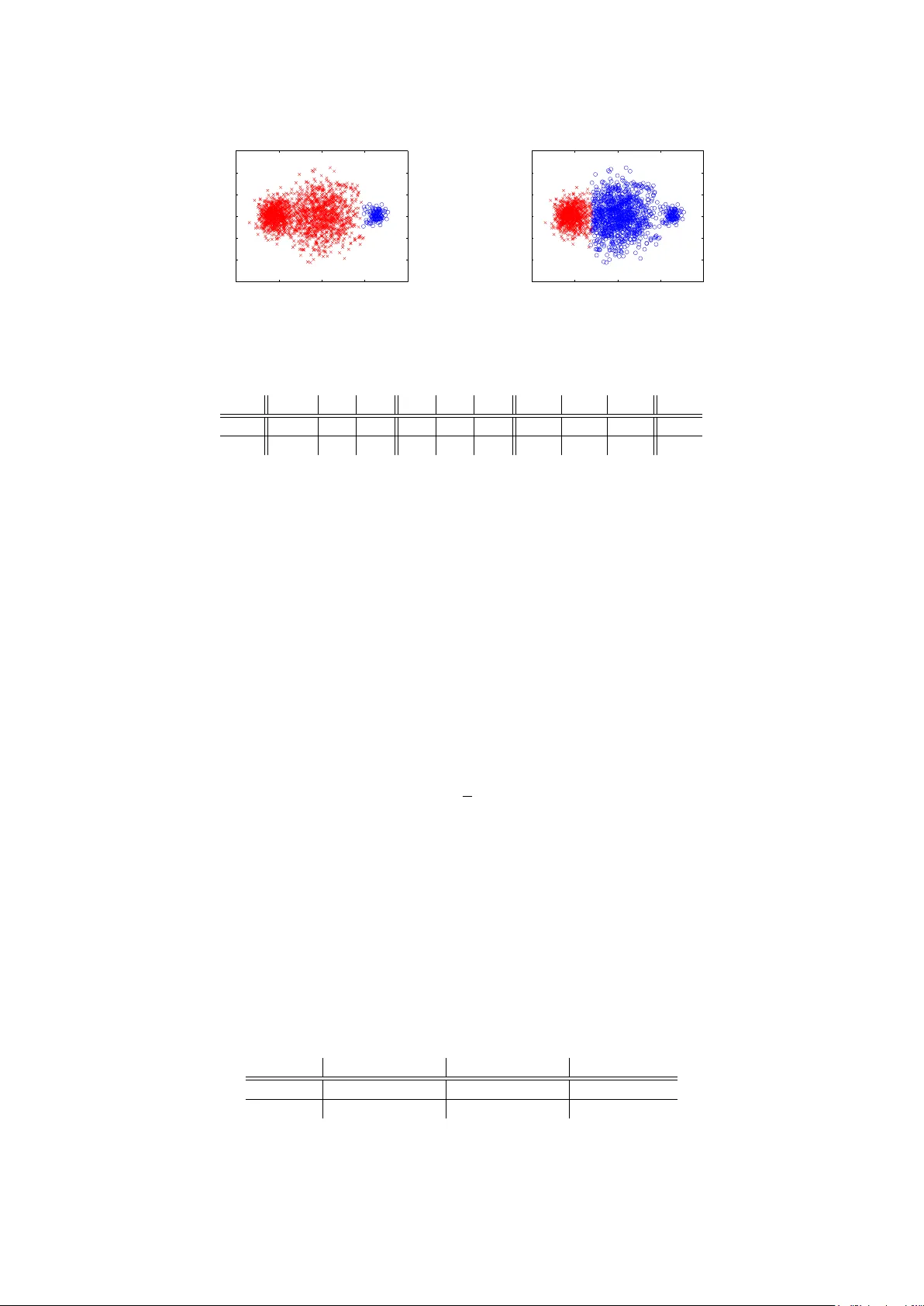
Ho w the result of graph clustering metho ds dep ends on the construction of the graph Markus Maier Max Planc k Institute for Biological Cyb ernetics, T ¨ ubingen, German y mmaier@tuebingen.mpg.de Ulrik e von Luxburg (Corresponding author) Max Planc k Institute for Biological Cyb ernetics, T ¨ ubingen, German y ulrike.luxburg@tuebingen.mpg.de Matthias Hein Saarland Univ ersity , Saarbr ¨ uc ken, German y hein@cs.uni-sb.de Octob er 24, 2018 Abstract W e study the scenario of graph-based clustering algorithms suc h as sp ectral clustering. Giv en a set of data points, one ﬁrst has to construct a graph on the data p oin ts and then apply a graph clustering algorithm to ﬁnd a suitable partition of the graph. Our main question is if and ho w the construction of the graph (choice of the graph, c hoice of parameters, choice of weigh ts) inﬂuences the outcome of the ﬁnal clustering result. T o this end we study the con vergence of cluster qualit y measures suc h as the normalized cut or the Cheeger cut on v arious kinds of random geometric graphs as the sample size tends to inﬁnity . It turns out that the limit v alues of the same ob jective function are systematically diﬀerent on diﬀeren t t yp es of graphs. This implies that clustering results systematically dep end on the graph and can be v ery diﬀeren t for diﬀerent types of graph. W e pro vide examples to illustrate the implications on spectral clustering. 1 In tro duction No wada ys it is v ery popular to represent and analyze statistical data using random graph or net work mo dels. The vertices in such a graph corresp ond to data p oin ts, whereas edges in the graph indicate that the adjacent v ertices are “similar” or “related” to each other. In this pap er w e consider the problem of data clustering in a random geometric graph setting. W e are giv en a sample of p oin ts dra wn from some underlying probability distribution on a metric space. The goal is to cluster the sample p oints in to “meaningful groups”. A standard pro cedure is to ﬁrst transform the data to a neigh b orhoo d graph, for example a k -nearest neigh b or graph. In a second step, the cluster structure is then extracted from the graph: clusters correspond to regions in the graph that are tigh tly connected within themselves and only sparsely connected to other clusters. There already exist a couple of pap ers that study statistical prop erties of this pro cedure in a particular setting: when the true underlying clusters are deﬁned to b e the connected components of a density level set in the underlying space. In his setting, a test for detecting cluster structure and outliers is proposed in Brito et al. (1997). In Biau et al. (2007) the authors build a neigh b orhoo d graph in such a wa y that its connected components conv erge to the underlying true clusters in the data. Maier et al. (2009a) compare the prop erties of diﬀerent random graph models for identifying clusters of the density level sets. 1 While the deﬁnition of clusters as connected comp onen ts of level sets is app ealing from a theoretical p oin t of view, the corresp onding algorithms are often too simplistic and only mo derately successful in practice. F rom a practical p oin t of view, clustering metho ds based on graph partitioning algo- rithms are more robust. Clusters do not hav e to b e perfectly disconnected in the graph, but are allo wed to hav e a small num b er of connecting edges b etw een them. Graph partitioning methods are widely used in practice. The most prominen t algorithm in this class is sp ectral clustering, whic h optimizes the normalized cut (NCut) ob jective function (see b elo w for exact deﬁnitions, and v on Luxburg (2007) for a tutorial on sp ectral clustering). It is already known under what circumstances sp ectral clustering is statistically consistent (von Luxburg et al., 2008). Ho wev er, there is one imp ortan t open question. When applying graph-based metho ds to given sets of data p oin ts, one obviously has to build a graph ﬁrst, and there are several imp ortan t choices to b e made: the type of the graph (for example, k -nearest neigh b or graph, the r -neigh b orhoo d graph or a Gaussian similarity graph), the connectivity parameter ( k or r or σ , resp ectiv ely) and the w eigh ts of the graph. Making such c hoices is not so diﬃcult in the domain of supervised learning, where parameters can b e set using cross-v alidation. How ever, it poses a serious problem in unsup ervised learning. While diﬀeren t researc hers use diﬀerent heuristics and their “gut feeling” to set these parameters, neither systematic empirical studies hav e b een conducted (for example, how sensitive the results are to the c hoice of graph parameters), nor do theoretical results exist which lead to w ell-justiﬁed heuristics. In this pap er w e study the question if and how the results of graph-based clustering algorithms are aﬀected by the graph type and the parameters that are chosen for the construction of the neigh b orho od graph. W e fo cus on the case where the b est clustering is deﬁned as the partition that minimizes the normalized cut (Ncut) or the Cheeger cut. Our theoretical setup is as follo ws. In a ﬁrst step w e ignore the problem of actually ﬁnding the optimal partition. Instead we ﬁx some partition of the underlying space and consider it as the “true” partition. F or any ﬁnite set of p oin ts drawn from the underlying space we consider the clustering of the p oin ts that is induced by this underlying partition. Then w e study the conv ergence of the NCut v alue of this clustering as the sample size tends to inﬁnit y . W e in vestigate this question on diﬀeren t kinds of neighborho o d graphs. Our ﬁrst main result is that depending on the t yp e of graph, the clustering qualit y measure conv erges to diﬀerent limit v alues. F or example, depending on whether we use the kNN graph or the r -graph, the limit functional in tegrates ov er diﬀeren t p o w ers of the density . F rom a statistical p oin t of view, this is very surprising b ecause in many other resp ects, the kNN graph and the r -graph b eha ve v ery similar to each other. Just consider the related problem of density estimation. Here, b oth the k -nearest neighbor density estimate and the estimate based on the degrees in the r -graph conv erge to the same limit, namely the true underlying density . So it is far from obvious that the NCut v alues w ould conv erge to diﬀerent limits. In a second step we then relate these results to the setting where we optimize o ver all partitions to ﬁnd the one that minimizes the NCut. W e can show that the results from the ﬁrst part can lead to the eﬀect that the minimizer of NCut on the kNN graph is diﬀerent from the minimizer of NCut on the r -graph or on the complete graph with Gaussian w eigh ts. This eﬀect can also b e studied in practical examples. First, we give examples of w ell-clustered distributions (mixtures of Gaussians) where the optimal limit cut on the kNN graph is diﬀeren t from the one on the r -neigh b orhoo d graph. The optimal limit cuts in these examples can b e computed analytically . Next w e can demonstrate that this eﬀect can already been observed on ﬁnite samples from these distributions. Given a ﬁnite sample, running normalized spectral clustering to optimize Ncut leads to systematically diﬀeren t results on the kNN graph than on the r -graph. This sho ws that our results are not only of theoretical interest, but that they are highly relev ant in practice. In the following section w e formally deﬁne the graph clustering qualit y measures and the neigh b or- ho od graph types w e consider in this pap er. F urthermore, we introduce the notation and tec hnical assumptions for the rest of the pap er. In Section 3 w e present our main results on the con vergence of NCut and the CheegerCut on diﬀeren t graphs. In Section 4 we show that our ﬁndings are not only of theoretical in terest, but that they also inﬂuence concrete algorithms such as sp ectral clustering in practice. All pro ofs are deferred to Section 6. Note that a small part of the results of this pap er has already b een published in Maier et al. (2009b). 2 2 Deﬁnitions and assumptions Giv en a directed graph G = ( V , E ) with w eights w : E → R and a partition of the no des V in to ( U, V \ U ) we deﬁne cut( U, V \ U ) = X u ∈ U,v ∈ V \ U ( w ( u, v ) + w ( v , u )) , and vol( U ) = P u ∈ U,v ∈ V w ( u, v ). If G is an undirected graph we replace the ordered pair ( u, v ) in the sums by the unordered pair { u, v } . Note that b y doing so we count eac h edge twice in the undirected graph. This introduces a constant of tw o in the limits but it has the adv antage that there is no need to distinguish in the formulation of our results betw een directed and undirected graphs. In tuitively , the cut measures ho w strong the connection betw een the diﬀeren t clusters in the clus- tering is, whereas the v olume of a subset of the no des measures the “weigh t” of the subset in terms of the edges that originate in it. An ideal clustering w ould ha ve a low cut and balanced clusters, that is clusters with similar volume. The graph clustering quality measures that we use in this pap er, the normalized cut and the Cheeger cut, formalize this trade-oﬀ in sligh tly diﬀeren t wa ys: The normalized cut is deﬁned b y NCut( U, V \ U ) = cut( U, V \ U )  1 v ol( U ) + 1 v ol( V \ U )  , (1) whereas the Cheeger cut is deﬁned by CheegerCut( U, V \ U ) = cut( U, V \ U ) min { v ol( U ) , v ol( V \ U ) } . (2) These deﬁnitions are useful for general weigh ted graphs and general partitions. As was said in the b eginning w e wan t to study the v alues of NCut and CheegerCut on neighborho o d graphs on sample points in Euclidean space and for partitions of the no des that are induced b y a h yp erplane S in R d . The t wo halfspaces b elonging to S are denoted by H + and H − . Having a neigh b orhoo d graph on the sample p oin ts { x 1 , . . . , x n } , the partition of the no des induced by S is ( { x 1 , . . . , x n } ∩ H + , { x 1 , . . . , x n } ∩ H − ). In the rest of this paper for a given neighborho o d graph G n w e set cut n = cut( { x 1 , . . . , x n } ∩ H + , { x 1 , . . . , x n } ∩ H − ). Similarly , for H = H + or H = H − w e set v ol n ( H ) = v ol( { x 1 , . . . , x n } ∩ H + ). Accordingly w e deﬁne NCut n and CheegerCut n . In the following we introduce the diﬀerent types of neigh b orho od graphs and weigh ting schemes that are considered in this pap er. The graph t yp es are: • The k -ne ar est neighb or ( kNN ) gr aphs , where the idea is to connect each point to its k nearest neigh b ors. How ever, this yields a directed graph, since the k -nearest neighbor relationship is not symmetric. If w e w ant to construct an undirected kNN graph we can choose b et w een the mutual kNN graph, where there is an edge betw een tw o p oin ts if both p oin ts are am ong the k nearest neighbors of the other one, and the symmetric kNN graph, where there is an edge b etw een tw o p oin ts if only one p oin t is among the k nearest neighbors of the other one. In our proofs for the limit expressions it will become clear that these do not diﬀer betw een the diﬀerent types of kNN graphs. Therefore, we do not distinguish b et w een them in the statemen t of the theorems, but rather speak of “the kNN graph”. • The r -neighb orho o d gr aph , where a radius r is ﬁxed and t wo p oin ts are connected if their distance do es not exceed the threshold radius r . Note that due to the symmetry of the distance we do not hav e to distinguish betw een directed and undirected graphs. • The c omplete weighte d gr aph , where there is an edge b etw een each pair of distinct no des (but no lo ops). Of course, in general w e would not consider this graph a neighborho o d graph. Ho wev er, if the weigh t function is chosen in such a wa y that the w eights of edges b et ween 3 nearb y no des are high and the w eigh ts b et ween p oints far aw a y from eac h other are almost negligible, then the b eha vior of this graph should b e similar to that of a neighborho o d graph. One such weigh t function is the Gaussian w eight function, whic h we introduce below. The w eights that are used on neigh b orho od graphs usually dep end on the distance of the end no des of the edge and are non-increasing. That is, the weigh t w ( x i , x j ) of an edge ( x i , x j ) is giv en b y w ( x i , x j ) = f (dist( x i , x j )) with a non-increasing weigh t function f . The weigh t functions we consider here are the unit weight function f ≡ 1, which results in the unw eighted graph, and the Gaussian weight function f ( u ) = 1 (2 π σ 2 ) d/ 2 exp  − 1 2 u 2 σ 2  with a parameter σ > 0 deﬁning the bandwidth. Of course, not every weigh ting scheme is suitable for every graph type. F or example, as mentioned ab o v e, w e would hardly consider the complete graph with unit weigh ts a neighborho o d graph. Therefore, we only consider the Gaussian w eigh t function for this graph. On the other hand, for the kNN graph and the r -neigh b orho od graph with Gaussian weigh ts there are tw o “mec hanisms” that reduce the inﬂuence of far-aw ay nodes: ﬁrst the fact that far-aw ay nodes are not connected to each other b y an edge and second the decay of the w eight function. In fact, it turns out that the limit expressions we study dep end on the interpla y b et w een these tw o mechanisms. Clearly , the decay of the weigh t function is gov erned by the parameter σ . F or the r -neigh b orhoo d graph the radius r limits the length of the edges. Asymptotically , giv en sequences ( σ n ) n ∈ N and ( r n ) n ∈ N of bandwidths and radii w e distinguish betw een the follo wing t w o cases: • the b andwidth σ n is dominate d by the r adius r n , that is σ n /r n → 0 for n → ∞ , • the r adius r n is dominate d by the b andwidth σ n , that is r n /σ n → 0 for n → ∞ . F or the kNN graph we cannot giv e a radius up to which p oin ts are connected by an edge, since this radius for each p oin t is a random v ariable that dep ends on the positions of all the sample points. Ho wev er, it is p ossible to show that for a p oin t in a region of constant density p the k n -nearest neigh b or radius is concentrated around d p k n / (( n − 1) η d p ), where η d denotes the volume of the unit ball in Euclidean space R d . That is, the kNN radius decays to zero with the rate d p k n /n . In the following it is conv enien t to set for the kNN graph r n = d p k n /n , noting that this is not the k -nearest neighbor radius of any p oint but only its deca y rate. Using this “radius” we distinguish b et w een the same t w o cases of the ratio of r n and σ n as for the r -neigh b orhoo d graph. F or the sequences ( r n ) n ∈ N and ( σ n ) n ∈ N w e alw a ys assume r n → 0, σ n → 0 and nr n → ∞ , nσ n → ∞ for n → ∞ . F urthermore, for the parameter sequence ( k n ) n ∈ N of the kNN graph we alwa ys assume k n /n → 0, whic h corresponds to r n → 0, and k n / log n → ∞ . In the rest of this pap er we denote b y L d the Leb esgue measure in R d . F urthermore, let B ( x, r ) denote the closed ball of radius r around x and η d = L d ( B (0 , 1)), where we set η 0 = 1. W e make the follo wing general assumptions in the whole pap er: • The data p oints x 1 , ..., x n ar e dr awn indep endently fr om some density p on R d . The me asur e on R d that is induc e d by p is denote d by µ ; that me ans, for a me asur able set A ⊆ R d we set µ ( A ) = R A p ( x ) d x . • The density p is b ounde d fr om b elow and ab ove, that is 0 < p min ≤ p ( x ) ≤ p max . In p articular, it has c omp act supp ort C . • In the interior of C , the density p is twic e diﬀer entiable and k∇ p ( x ) k ≤ p 0 max for a p 0 max ∈ R and al l x in the interior of C . • The cut hyp erplane S splits the sp ac e R d into two halfsp ac es H + and H − (b oth including the hyp erplane S ) with p ositive pr ob ability masses, that is µ ( H + ) > 0 , µ ( H − ) > 0 . The normal of S p ointing towar ds H + is denote d by n S . 4 • If d ≥ 2 the b oundary ∂ C is a c omp act, smo oth ( d − 1) -dimensional surfac e with minimal curvatur e r adius κ > 0 , that is the absolute values of the princip al curvatur es ar e b ounde d by 1 /κ . We denote by n x the normal to the surfac e ∂ C at the p oint x ∈ ∂ C . F urthermor e, we c an ﬁnd c onstants γ > 0 and r γ > 0 such that for al l r ≤ r γ we have L d ( B ( x, r ) ∩ C ) ≥ γ L d ( B ( x, r )) for al l x ∈ C . • If d ≥ 2 we c an ﬁnd an angle α ∈ (0 , π / 2) such that |h n S , n x i| ≤ cos α for al l x ∈ S ∩ ∂ C . If d = 1 we assume that (the p oint) S is in the interior of C . The assumptions on the b oundary ∂ C are necessary in order to b ound the inﬂuence of p oints that are close to the b oundary . The problem with these p oin ts is that the density is not approximately uniform inside small balls around them. Therefore, we cannot ﬁnd a goo d estimate of their kNN radius and on their contribution to the cut and the v olume. Under the assumptions abov e we can neglect these points. 3 Main results: Limits of the qualit y measures NCut and CheegerCut As we can see in Equations (1) and (2) the deﬁnitions of NCut and CheegerCut rely on the cut and the v olume. Therefore, in order to study the con vergence of NCut and CheegerCut it seems reasonable to study the conv ergence of the cut and the v olume ﬁrst. In Section 6 the Corollaries 1-3 and the Corollaries 4-6 state the conv ergence of the cut and the volume on the kNN graphs. The Corollaries 7-10 state the conv ergence of the cut on the r -graph and the complete weigh ted graph, whereas the Corollaries 11-14 state the conv ergence of the volume on the same graphs. These corollaries sho w that there are scaling sequences ( s cut n ) n ∈ N and ( s vol n ) n ∈ N that dep end on n , r n and the graph type suc h that, under certain conditions, almost surely  s cut n  − 1 cut n → C utLim and  s vol n  − 1 v ol n ( H ) → V olLim ( H ) for n → ∞ , where C utLim ∈ R ≥ 0 and V ol Lim ( H + ) , V ol Lim ( H − ) ∈ R > 0 are constan ts depending only on the density p and the hyperplane S . Ha ving deﬁned these limits we deﬁne, analogously to the deﬁnitions in Equations (1) and (2), the limits of NCut and CheegerCut as N C utLim = C utLim V olLim ( H + ) + C utLim V olLim ( H − ) (3) and C heeg erC utLim = C utLim min { V ol Lim ( H + ) , V olLim ( H − ) } . (4) In our follo wing main theorems w e show the conditions under whic h we ha ve for n → ∞ almost sure conv ergence of s vol n s cut n NCut n → N C utLim and s vol n s cut n CheegerCut n → C heeg er C utLim. F urthermore, for the unw eighted r -graph and kNN-graph and for the complete weigh ted graph with Gaussian weigh ts w e state the optimal conv e rgence rates, where “optimal” means the b est trade-oﬀ b et ween our b ounds for diﬀeren t quan tities derived in Section 6. Note that we will not pro ve the following theorems here. Rather the proof of Theorem 1 can b e found in Section 6.2.4, whereas the proofs of Theorems 2 and 3 can b e found in Section 6.3.3. 5 The cut in the kNN -graph and the r -graph W eigh ting s cut n C utLim kNN-graph C utLim r -graph un weigh ted n 2 r d +1 n 2 η d − 1 ( d +1) η 1+1 /d d R S p 1 − 1 /d ( s ) d s 2 η d − 1 d +1 R S p 2 ( s ) d s w eighted r n /σ n → ∞ n 2 σ n 2 √ 2 π R S p 2 ( s ) d s 2 √ 2 π R S p 2 ( s ) d s w eighted r n /σ n → 0 σ − d n n 2 r d +1 n 2 η d − 1 η − 1 − 1 /d d ( d +1)(2 π ) d/ 2 R S p 1 − 1 /d ( s ) d s 2 η d − 1 ( d +1)(2 π ) d/ 2 R S p 2 ( s ) d s The cut in the complete weigh ted graph W eigh ting s cut n C utLim in complete weigh ted graph w eighted n 2 σ n 2 √ 2 π R S p 2 ( s ) d s The volume in the kNN -graph and the r -graph W eigh ting s vol n V olLim ( H ) kNN-graph V olLim ( H ) r -graph un weigh ted n 2 r d n R H p ( x ) d x η d R H p 2 ( x ) d x w eighted, r n /σ n → ∞ n 2 R H p 2 ( x ) d x R H p 2 ( x ) d x w eighted, r n /σ n → 0 σ − d n n 2 r d n 1 (2 π ) d/ 2 R H p ( x ) d x η d (2 π ) d/ 2 R H p 2 ( x ) d x The volume in the complete weigh ted graph W eigh ting s vol n V olLim in complete w eigh ted graph w eighted n 2 R H p 2 ( x ) d x T able 1: The scaling sequences and limit expression for the cut and the v olume in all the considered graph t yp es. In the limit expression for the cut the integral denotes the ( d − 1)-dimensional surface in tegral along the hyperplane S , whereas in the limit expressions for the v olume the in tegral denotes the Leb esgue in tegral o ver the halfspace H = H + or H = H − . Theorem 1 ( NCut and CheegerCut on the kNN -graph) F or a se quenc e ( k n ) n ∈ N with k n /n → 0 for n → ∞ let G n b e the k n -ne ar est neighb or gr aph on the sample x 1 , . . . , x n . Set XCut = NCut or X Cut = CheegerCut and let X C utLim denote the c orr esp onding limit as deﬁne d in Equations (3) and (4) . Set ∆ n =     s vol n s cut n X Cut n − X C utLim     . • L et G n b e the unweighte d kNN gr aph. If k n / √ n log n → ∞ in the c ase d = 1 and k n / log n → ∞ in the c ase d ≥ 2 we have ∆ n → 0 for n → ∞ almost sur ely. The optimal c onver genc e r ate is achieve d for k n = k 0 4 p n 3 log n in the c ase d = 1 and k n = k 0 n 2 / ( d +2) (log n ) d/ ( d +2) in the c ase d ≥ 2 . F or this choic e of k n we have ∆ n = O ( d +4 p log n/n ) in the c ase d = 1 and ∆ n = O ( d +2 p log n/n ) for d ≥ 2 . • L et G n b e the kNN -gr aph with Gaussian weights and supp ose r n ≥ σ α n for an α ∈ (0 , 1) . Then we have almost sur e c onver genc e of ∆ n → 0 for n → ∞ if k n / log n → ∞ and nσ d +1 n / log n → ∞ . • L et G n b e the kNN -gr aph with Gaussian weights and r n /σ n → 0 . Then we have almost sur e c onver genc e of ∆ n → 0 for n → ∞ if k n / √ n log n → ∞ in the c ase d = 1 and k n / log n → ∞ in the c ase d ≥ 2 . Theorem 2 ( NCut and CheegerCut on the r -graph) F or a se quenc e ( r n ) n ∈ N ⊆ R > 0 with r n → 0 for n → ∞ let G n b e the r n -neighb orho o d gr aph on the sample x 1 , . . . , x n . Set XCut = NCut or X Cut = CheegerCut and let X C utLim denote the c orr esp onding limit as deﬁne d in Equations (3) and (4) . Set ∆ n =     s vol n s cut n X Cut n − X C utLim     . 6 • L et G n b e unweighte d. Then ∆ n → 0 almost sur ely for n → ∞ if nr d +1 n / log n → ∞ . The optimal c onver genc e r ate is achieve d for r n = r 0 d +3 p log n/n for a suitable c onstant r 0 > 0 . F or this choic e of r n we have ∆ n = O ( d +3 p log n/n ) . • L et G n b e weighte d with Gaussian weights with b andwidth σ n → 0 and r n /σ n → ∞ for n → ∞ . Then ∆ n → 0 almost sur ely for n → ∞ if nσ d +1 n / log n → ∞ . • L et G n b e weighte d with Gaussian weights with b andwidth σ n → 0 and r n /σ n → 0 for n → ∞ . Then ∆ n → 0 almost sur ely for n → ∞ if nr d +1 n / log n → ∞ . The follo wing theorem presents the limit results for NCut and CheegerCut on the complete w eighted graph. One result that w e need in the pro of of this theorem is Corollary 8 on the con vergence of the cut. Note that in Naray anan et al. (2007) a similar cut conv ergence problem is studied for the case of the complete w eigh ted graph, and the scaling sequence and the limit diﬀer from ours. Ho wev er, the reason is that in that pap er the weighte d cut is considered, which can be written as f 0 L norm f , where L norm denotes the normalized graph Laplacian matrix and f is an n -dimensional v ector with f i = 1 if x i is in one cluster and f i = 0 if x i is in the other cluster. On the other hand, the standard cut, whic h w e consider in this paper, can b e written (up to a constan t) as f 0 L unnorm f , where L unnorm denotes the unnormalized graph Laplacian matrix. (F or the deﬁnitions of the graph Laplacian matrices and their relationship to the cut we refer the reader to v on Luxburg (2007).) Therefore, the t wo results do not contradict eac h other. Theorem 3 ( NCut and CheegerCut on the complete weigh ted graph) L et G n b e the c om- plete weighte d gr aph with Gaussian weights and b andwidth σ n on the sample p oints x 1 , . . . , x n . Set X Cut = NCut or X Cut = CheegerCut and let X C utLim denote the c orr esp onding limit as deﬁne d in Equations (3) and (4) . Set ∆ n =     s vol n s cut n X Cut n − X C utLim     . Under the c onditions σ n → 0 and nσ d +1 n / log n → ∞ we have almost sur ely ∆ n → 0 for n → ∞ . The optimal c onver genc e r ate is achieve d setting σ n = σ 0 d +3 p log n/n with a suitable σ 0 > 0 . F or this choic e of σ n the c onver genc e r ate is in O (((log n ) /n ) α/ ( d +3) ) for any α ∈ (0 , 1) . Let us decrypt these results and for simplicity fo cus on the cut v alue. When we compare the limits of the cut (cf. T able 1) it is striking that, depending on the graph type and the weigh ting scheme, there are tw o substan tially diﬀeren t limits: the limit R S p 2 ( s ) d s for the u nw eighted r -neigh b orho od graph, and the limit R S p 1 − 1 /d ( s ) d s for the un w eighted k -nearest neighbor graph. The limit of the cut for the complete w eighted graph with Gaussian weigh ts is the same as the limit for the un weigh ted r -neighborho o d graph. There is a simple reason for that: On b oth graph t yp es the weigh t of an edge only dep ends on the distance b et ween its end p oin ts, no matter where the p oin ts are. This is in c on trast to the kNN-graph, where the radius up to whic h a p oint is connected strongly dep ends on its location: If a p oint is in a region of high density there will be man y other p oints close b y , which means that the radius is small. On the other hand, this radius is large for p oin ts in low-densit y regions. F urthermore, the Gaussian weigh ts decline v ery rapidly with the distance, dep ending on the parameter σ . That is, σ pla ys a similar role as the radius r for the r -neighborho o d graph. The tw o t yp es of r -neigh b orho od graphs with Gaussian w eights hav e the same limit as the un- w eighted r -neigh b orhoo d graph and the complete weigh ted graph with Gaussian weigh ts. When w e compare the scaling sequences s cut n it turns out that in the case r n /σ n → ∞ this sequence is the same as for the complete w eighted graph, whereas in the case r n /σ n → 0 we ha ve s cut n = n 2 r d +1 n /σ d n , whic h is the same sequence as for the unw eighted r -graph corrected by a factor of σ − d n . In fact, these eﬀects are easy to explain: If r n /σ n → ∞ then the edges which we hav e to remo v e from the complete w eighted graph in order to obtain the r n -neigh b orho od graph hav e a v ery small weigh t and their con tribution to the v alue of the cut can b e neglected. Therefore this graph behav es like the complete w eighted graph with Gaussian weigh ts. On the other hand, if r n /σ n → 0 then all the 7 −1 0 1 2 0 0.5 1 Density example 1 −2 −1 0 1 2 0 0.5 1 Density example 2 (informative dimension only) Figure 1: Densities in the examples. In the tw o-dimensional case, w e plot the informative dimension (marginal ov er the other dimensions) only . The dashed blue vertical line depicts the optimal limit cut of the r -graph, the solid red vertical line the optimal limit cut of the kNN graph. edges that remain in the r n -neigh b orho od graph hav e approximately the same weigh t, namely the maxim um of the Gaussian w eight function, whic h is linear in σ − d n . Similar eﬀects can b e observed for the k -nearest neighbor graphs. The limits of the unw eighted graph and the graph with Gaussian weigh t and r n /σ n → 0 are iden tical (up to constants) and the scaling sequence has to correct for the maximum of the Gaussian weigh t function. How ever, the limit for the kNN-graph with Gaussian w eights and r n /σ n → ∞ is diﬀeren t: In fact, w e ha v e the same limit expression as for the complete w eighted graph with Gaussian weigh ts. The reason for this is the follo wing: Since r n is large compared to σ n at some p oin t all the k -nearest neighbor radii of the sample points are v ery large. Therefore, all the edges that are in the complete w eighted graph but not in the kNN graph hav e very lo w weigh ts and thus the limit of this graph b ehav es lik e the limit of the complete weigh ted graph with Gaussian weigh ts. Finally , w e w ould like to discuss the diﬀerence b et ween the tw o limit expressions, where as examples for the graphs we use only the un w eighted r -neighborho od grap h and the un w eighted kNN-graph. Of course, the results can be carried ov er to the other graph types. F or the cut we hav e the limits R S p 1 − 1 /d ( s ) d s and R S p 2 ( s ) d s . In dimension 1 the diﬀerence b et ween these expressions is most pronounced: The limit for the kNN graph do es not depend on the densit y p at all, whereas in the limit for the r -graph the exp onen t of p is 2, indep endent of the dimension. Generally , the limit for the r -graph seems to b e more sensitive to the absolute v alue of the density . This can also b e seen for the volume: The limit expression for the kNN graph is R H p ( x ) d x , which do es not depend on the absolute v alue of the density at all, but only on the probability mass in the halfspace H . This is diﬀerent for the unw eighted r -neigh b orho od graph with the limit expression R H p 2 ( x ) d x . 4 Examples where diﬀeren t limits of Ncut lead to diﬀeren t optimal cuts In Theorems 1-3 we hav e prov ed that the limit expressions for NCut and CheegerCut are diﬀerent for diﬀeren t kinds of neighborho od graphs. In fact, apart from constants there are t wo limit expressions: that of the unw eigh ted kNN-graph, where the exponent of the densit y p in the limit in tegral for the cut is 1 − 1 /d and for the v olume is 1, and that of the unw eighted r -neighborho od graph, where the exponent in the limit of the cut is 2 and in the limit of the v ol is 1. Therefore, w e consider here only the unw eighted kNN-graph and the unw eigh ted r -neighborho o d graph. In this section we sho w that the diﬀerence b etw een the limit expressions is more than a mathemat- ical subtlety without practical relev ance: If we select an optimal cut based on the limit criterion for the kNN graph we can obtain a diﬀeren t result than if we use the limit criterion based on the r -neigh b orhoo d graph. Consider Gaussian mixture distributions in one (Example 1) and in tw o dimensions (Example 2) of the form P 3 i =1 α i N ([ µ i , 0 , . . . , 0] , σ i I ) whic h are set to zero where they are below a threshold θ and prop erly rescaled. The speciﬁc parameters in one and t wo dimensions are 8 −2 −1 0 1 2 −1.5 −1 −0.5 0 0.5 1 1.5 r−graph, n=2000, r=150−NN radius −2 −1 0 1 2 −1.5 −1 −0.5 0 0.5 1 1.5 kNN graph, n=2000, k=150 Figure 2: Results of sp ectral clustering in t wo dimensions, for the un weigh ted r -graph (left) and the unw eighted kNN graph (righ t) dim µ 1 µ 2 µ 3 σ 1 σ 2 σ 3 α 1 α 2 α 3 θ 1 0 0.5 1 0.4 0.1 0.1 0.66 0.17 0.17 0.1 2 − 1 . 1 0 1 . 3 0.2 0.4 0.1 0.4 0.55 0.05 0.01 Plots of the densities of Example 1 and 2 can b e seen in Figure 1. W e ﬁrst in vestigate the theoretic limit cut v alues, for hyperplanes whic h cut p erpendicular to the ﬁrst dimension (which is the “informativ e” dimension of the data). F or the chosen densities, the limit NCut expressions from Theorems 1 and 2 can b e computed analytically and optimized ov er the c hosen hyperplanes. The solid red line in Figure 1 indicates the p osition of the minimal v alue for the kNN-graph case, whereas the dashed blue line indicates the the p osition of the minimal v alue for the r -graph case. Up to now w e only compared the limits of diﬀeren t graphs with eac h other, but the question is, whether the eﬀects of these limits can b e observ ed even for ﬁnite sample sizes. In order to in vestigate this question we applied normalized sp ectral clustering (cf. v on Luxburg (2007)) to sample data sets of n = 2000 p oints from the mixture distribution ab o ve. W e used the unw eigh ted r -graph and the un w eighted symmetric k -nearest neigh bor graph. W e tried a range of reasonable v alues for the parameters k and r and the results we obtained w ere stable ov er a range of parameters. Here we present the results for the 30- (for d = 1) and the 150-nearest neighbor graphs (for d = 2) and the r -graphs with corresp onding parameter r , that is r was set to be the mean 30- and 150- nearest neighbor radius. Diﬀeren t clusterings are compared using the minimal matc hing distance: d M M (Clust 1 , Clust 2 ) = min π 1 n n X i =1 1 Clust 1 ( x i ) 6 = π (Clust 2 ( x i )) where the minimum is tak en ov er all p erm utations π of the lab els. In the case of tw o clusters, this distance corresp onds to the 0-1-loss as used in classiﬁcation: a minimal matching distance of 0 . 35, sa y , means that 35% of the data p oin ts lie in diﬀeren t clusters. In our sp ectral clustering exp erimen t, we could observe that the clusterings obtained by sp ectral clustering are usually v ery close to the theoretically optimal h yp erplane splits predicted by theory (the minimal matc hing distances to the optimal hyperplane splits were alwa ys in the order of 0.03 or smaller). As predicted b y theory , the tw o types of graph giv e diﬀeren t cuts in the data. An illustration of this phenomenon for the case of dimension 2 can b e found in Figure 2. T o give a quantitativ e ev aluation of this phenomenon, we computed the mean minimal matching distances b etw een clusterings obtained b y the same type of graph ov er the diﬀerent samples (denoted d kNN and d r ), and the mean diﬀerence d kNN − r b et w een the clusterings obtained b y diﬀeren t graph t yp es: Example d kNN d r d kNN − r 1 dim 0 . 0005 ± 0 . 0006 0 . 0003 ± 0 . 0004 0 . 346 ± 0 . 063 2 dim 0 . 005 ± 0 . 0023 0 . 001 ± 0 . 001 0 . 49 ± 0 . 01 W e can see that for the same graph, the clustering results are v ery stable (diﬀerences in the order of 10 − 3 ) whereas the diﬀerences betw een the kNN graph and the r -neighborho o d graph are 9 0 0.2 0.4 0 2 4 6 8 Density example 3 0 0.2 0.4 0 50 100 kNN−graph, k=200 0 0.2 0.4 0 50 100 r−graph, r=200−NN radius Figure 3: The Example 3 with the sum of tw o Gaussians, that is tw o mo des of the densit y . In the left ﬁgure the density with the optimal limit cut of the r -graph (dashed blue vertical line) and the optimal limit cut of the kNN graph (the solid red vertical line) is depicted. The tw o ﬁgures on the right sho w the histograms of the cluster b oundary ov er 100 iterations for the unw eigh ted r -neigh b orhoo d and kNN-graphs. substan tial (0.35 and 0.49, resp ectiv ely). This diﬀerence is exactly the one induced b y assigning the middle mode of the densit y to diﬀeren t clusters, whic h is the eﬀect predicted by theory . It is tempting to conjecture that in Example 1 and 2 the tw o diﬀerent limit solutions and their impact on sp ectral clustering might arise due to the fact that the num b er of Gaussians and the n umber of clusters we are lo oking for do not coincide. Y et the follo wing Example 3 shows that this is not the case: for a density in one dimension as ab o ve but with only tw o Gaussians with parameters µ 1 µ 2 σ 1 σ 2 α 1 α 2 θ 0.2 0.4 0.05 0.03 0.8 0.2 0.1 the same eﬀects can be observ ed. The densit y is depicted in the left plot of Figure 3. In this example w e draw a sample of 2000 p oints from this densit y and compute the sp ectral clustering of the p oin ts, once with the unw eighted kNN-graph and once with the unw eigh ted r - graph. In one dimension w e can compute the place of the b oundary betw een t wo clu sters, that is the middle betw een the rightmost p oin t of the left cluster and the leftmost p oin t of the right cluster. W e did this for 100 iterations and plotted histograms of the location of the cluster b oundary . In the middle and the righ t plot of Figure 3 we see that these coincide with the optimal cut predicted b y theory . 5 Outlo ok In this pap er we hav e in vestigated the inﬂuence of the graph construction on the graph-based clustering measures normalized cut and Cheeger cut. W e hav e seen that dep ending on the type of graph and the weigh ts, the clustering quality measures conv erge to diﬀeren t limit results. This means that ultimately , the question ab out the “b est NCut” or “b est Cheeger cut” clustering, giv en inﬁnite amount of data, has diﬀerent answers, depending on which underlying graph we use. This observ ation op ens Pandora’s b o x on clustering criteria: the “meaning” of a clustering criterion do es not only depend on the exact deﬁnition of the criterion itself, but also on how the graph on the ﬁnite sample is constructed. This means that one graph clustering qualit y measure is not just “one well-deﬁned criterion” on the underlying space, but it corresp onds to a whole bunch of criteria, whic h diﬀer dep ending on the underlying graph. More sloppy: A clustering qualit y measure applied to one neighborho o d graph do es something diﬀeren t in terms of partitions of the underlying space than the same qualit y measure applied to a diﬀeren t neigh b orhoo d graph. This sho ws that these criteria cannot b e studied isolated from the graph they are applied to. F rom a theoretical side, there are several directions in whic h our work can be improv ed. In this pap er w e only consider partitions of Euclidean space that are deﬁned b y hyperplanes. This restriction is made in order to keep the proofs reasonably simple. How ever, we are conﬁden t that similar results could b e prov en for arbitrary smo oth surfaces. 10 Another extension would b e to obtain uniform conv ergence results. Here one has to tak e care that one uses a suitably restricted class of candidate surfaces S (note that uniform conv ergence results o ver the set of all partitions of R d are imp ossible, cf. Bub ec k and v on Luxburg (2009)). This result would b e esp ecially useful, if there existed a practically applicable algorithm to compute the optimal surface out of the set of all candidate surfaces. F or practice, it will be important to study ho w the diﬀeren t limit results inﬂuence clustering results. So far, we do not hav e muc h in tuition about when the diﬀeren t limit expressions lead to diﬀeren t optimal solutions, and when these solutions will show up in practice. The examples w e provided ab o v e already show that diﬀerent graphs indeed can lead to systematically diﬀerent clusterings in practice. Gaining more understanding of this eﬀect will b e an imp ortan t direction of research if one wan ts to understand the nature of diﬀeren t graph clustering quality measures. 6 Pro ofs In many of the pro ofs that are to follow in this section a lot of technique is inv olved in order to come to terms with problems that arise due to eﬀects at the b oundary of our supp ort C and to the non-uniformit y of the density p . How ever, if these technicalities are ignored, the basic ideas of the pro ofs are simple to e xplain and they are similar for the diﬀeren t types of neighborho o d graphs. In Section 6.1 we discuss these ideas without the technical ov erhead and deﬁne some quan tities that are necessary for the form ulation of our results. In Section 6.2 we presen t the results for the k -nearest neigh b or graph and in Section 6.3 w e present those for the r -graph and the complete weigh ted graph. Each of these sections consists of three parts: the ﬁrst is devoted to the cut, the second is devoted to the v olume, and in the third we pro of the main theorem for the considered graphs using the results for the cut and the v olume. The sections on the con vergence of the cut and the volume alwa ys follow the same scheme: First, a prop osition concerning the con vergence of the cut or the v olume for general monotonically de- creasing weigh t functions is given. Using this general prop osition the results for the sp eciﬁc weigh t functions we consider in this pap er follo w as corollaries. Since the basic ideas of our pro ofs are the same for all the diﬀeren t graphs, it is not w orth repeating the same steps for all the graphs. Therefore, we decided to giv e detailed proofs for the k -nearest neigh b or graph, which is the most diﬃcult case. The r -neigh b orho od graph and the complete w eighted graph can be treated together and w e mainly discuss the diﬀerences to the pro of for the kNN graph. The limits of the cut and the v olume for general w eigh t function are expressed in terms of certain in tegrals of the weigh t function o v er “caps” and “balls”, which are explained later. F or a sp eciﬁc w eight function these integrals ha ve to b e ev aluated. This is done in the lemmas in Section 6.4. F urthermore, this section contains a tec hnical lemma that helps us to con trol b oundary eﬀects. 6.1 Basic ideas In this section we present the ideas of our conv ergence pro ofs non-formally . W e fo cus here on NCut, but all the ideas can easily be carried ov er to the Cheeger cut. First step: De c omp ose NCut n into cut n and v ol n Under our general assumptions there exist constan ts c 1 , c 2 , c 3 , whic h may dep end on the limit v alues of the cut and the v olume, suc h that for suﬃciently large n     s vol n s cut n  cut n v ol n ( H + ) + cut n v ol n ( H − )  − C utLim V olLim ( H + ) + C utLim V olLim ( H − )     ≤ c 1     cut n s cut n − C utLim     | {z } cut term + c 2     v ol n ( H + ) s vol n − V olLim ( H + )     | {z } volume-term + c 3     v ol n ( H − ) s vol n − V olLim ( H − )     | {z } volume-term . 11 Se c ond step: Bias/varianc e de c omp osition of cut and volume terms In order to show the conv ergence of the cut-term w e do a bias/v ariance decomposition     cut n s cut n − C utLim     ≤     cut n s cut n − E  cut n s cut n      | {z } v ariance term +     E  cut n s cut n  − C utLim     | {z } bias term and sho w the con vergence to zero of these terms separately . Clearly , the same decomp osition can b e done for the volume terms. In the follo wing we call these terms the “bias term of the cut” and the “v ariance term of the cut” and similarly for the v olume. F or b oth, the cut and the v olume, there is one result in this section dealing with the conv ergence prop erties of the bias term and the v ariance term on eac h particular graph type and weigh ting sc heme. Thir d step: Use c onc entr ation of me asur e ine qualities for the varianc e term Bounding the deviation of a random v ariable from its exp ectation is a w ell-studied problem in statistics and there are a couple of so-called concen tration of measure inequalities that bound the probabilit y of a large deviation from the mean. In this pap er w e use McDiarmid’s inequalit y for the kNN graphs and a concentration of measure result for U -statistics by Ho eﬀding for the r -neigh b orhoo d graph and the complete weigh ted graph. The reason for this is that eac h of the graph types has its particular adv antages and disadv antages when it comes to the prerequisites for the concen tration inequalities: The adv antage of the kNN graph is that we can bound the degree of a no de linearly in the parameter k , whereas for the r -neighborho od graph we can b ound the degree only b y the trivial bound ( n − 1) and for the complete graph this bound is ev en attained. Therefore, using the same pro of as for the kNN-graph is sub optimal for the latter tw o graphs. On the other hand, in these graphs the connectivity b et ween p oin ts is not random given their p osition and it is alwa ys symmetric. This allows us to use a U -statistics argument, whic h cannot b e applied to the kNN-graph, since the connectivity there may b e unsymmetric (at least for the directed one) and the connectivit y betw een each tw o p oin ts depends on all the s ample p oin ts. Note that these results are of a probabilistic nature, that is we obtain results of the form Pr      cut n s cut n − E  cut n s cut n      > ε  ≤ p n , for a sequence ( p n ) of non-negativ e real num b ers. If for all ε > 0 the sum P ∞ i =1 p i is ﬁnite, then w e ha ve almost sure conv ergence of the v ariance term to zero b y the Borel-Can telli lemma. F ourth step: Bias of the cut term While all steps so far were pretty muc h standard, this part is the technically most c hallenging part of our conv ergence pro of. W e hav e to prov e the con vergence of E (cut n /s cut n ) to C utLim (and similarly for the volume). Omitting all tec hnical diﬃculties like b oundary eﬀects and the v ariability of the density , the basic ideas can b e describ ed in a rather simple manner. The ﬁrst idea is to break the cut down into the con tributions of eac h single edge. W e deﬁne a random v ariable W ij that attains the weigh t of the edge b et ween x i and x j , if these p oin ts are connected in the graph and on diﬀerent sides of the hyperplane S , and zero otherwise. By the linearit y of the expectation and the fact that the points are sampled i.i.d. E (cut n ) = n X i =1 n X j =1 j 6 = i E W ij = n ( n − 1) E W 12 . No w w e ﬁx the p ositions of the p oin ts x 1 = x and x 2 = y . In this case W ij can attain only tw o v alues: f n (dist( x, y )) if the p oints are connected and on diﬀerent sides of S , and zero otherwise. W e ﬁrst consider the r -neigh b orhoo d graph with parameter r n , since here the existence of an edge b et w een tw o p oin ts is determined b y their distance, and is not random as in the kNN graph. Two p oin ts are connected if their distance is not greater than r n and thus W ij = 0 if dist( x, y ) > r n . 12 F urthermore, W ij = 0 if x and y are on the same side of S . That is, for a p oin t x ∈ H + w e ha ve E ( W 12 | x 1 = x, x 2 = y ) = ( f n (dist( x, y )) if y is in the cap B ( x, r n ) ∩ H − 0 otherwise. By integrating ov er R d w e obtain E ( W 12 | x 1 = x ) = Z B ( x,r n ) ∩ H − f n (dist( x, y )) p ( y ) d y and denote the integral on the righ t hand side in the following b y g ( x ). In tegrating the conditional expectation ov er all p ossible p ositions of the p oin t x in R d giv es E ( W 12 ) = Z R d g ( x ) p ( x ) d x = Z H + g ( x ) p ( x ) d x + Z H − g ( x ) p ( x ) d x. W e only consider the in tegral o v er the halfspace H + here, since the other in tegral can be treated analogously . The imp ortant idea in the ev aluation of this integral is the follo wing: Instead of in tegrating ov er H + , we initially in tegrate ov er the hyperplane S and then, at eac h p oint s ∈ S , along the normal line through s , that is the line s + tn S for all t ∈ R ≥ 0 . This leads to Z H + g ( x ) p ( x ) d x = Z S Z ∞ 0 g ( s + tn S ) p ( s + tn S ) d t d s. S H − H + s s + tn S r n Figure 4: Integration along the normal line through s . Obviously , for t ≥ r n the intersection B ( s + tn S , r n ) ∩ H − is empt y and therefore g ( s + tn S ) = 0. F or 0 ≤ t < r n the points in the cap are close to s and therefore the densit y in the cap is approximately p ( s ). This in tegration is illustrated in Figure 4. It h as t wo adv antages: First, if x is far enough from S (that is, dist( x, s ) > r n for all s ∈ S ), then g ( x ) = 0 and the corresp onding terms in the in tegral v anish. Second, if x is close to s ∈ S and the radius r n is small, then the density on the ball B ( x, r n ) can be considered appro ximately uniform, that is w e assume p ( y ) = p ( s ) for all y ∈ B ( x, r n ). Th us, Z ∞ 0 g ( s + tn S ) p ( s + tn S ) d t = Z r n 0 g ( s + tn S ) p ( s + tn S ) d t = p ( s ) Z r n 0 g ( s + tn S ) d t = p 2 ( s ) Z r n 0 Z B ( x,r n ) ∩ H − f n (dist( x, y )) d y d t = η d − 1 Z r n 0 u d f n ( u ) d u p 2 ( s ) where the last step follo ws with Lemma 3. Since this integral of the weigh t function f n o ver the “caps” plays suc h an important role in the deriv ation of our results w e in tro duce a sp ecial notation for it: F or a radius r ∈ R ≥ 0 and q = 1 , 2 w e deﬁne F ( q ) C ( r ) = η d − 1 Z r 0 u d f q n ( u ) d u. 13 Although these in tegrals also dep end on n w e do not mak e this dep endence explicit. In fact, the parameter r is replaced by the radius r n in the case of the r -neighborho od graph or b y a diﬀerent graph parameter dep ending on n for the other neigh b orhoo d graphs. Therefore the dep endence of F ( q ) C ( r n ) on n will b e understo o d. Note that we allow the notation F ( q ) C ( ∞ ), if the indeﬁnite in tegral exists. The in tegral F ( q ) C for q = 2 is needed for the follo wing reason: F or the U -statistics b ound on the v ariance term w e do not only hav e to compute the exp ectation of W ij , but also their v ariance. But the v ariance can in turn b e b ounded b y the exp ectation of W 2 ij , whic h is expressed in terms of F (2) C ( r n ). In the r -neighborho od graph p oin ts are only connected within a certain radius r n , which means that to compute E ( W 12 | x 1 = x ) we only hav e to integrate o v er the ball B ( x, r n ), since all other p oin ts cannot b e connected to x 1 = x . This is clearly diﬀerent for the complete graph, where every p oin t is connected to ev ery other p oin t. The idea is to ﬁx a radius r n in suc h a wa y as to make sure that the contribution of edges to p oints outside B ( x, r n ) can b e neglected, because their w eight is small. Since W 12 = f n (dist( x 1 , x 2 )) if the p oin ts are on diﬀerent sides of S we ha ve for x ∈ H + E ( W 12 | x 1 = x ) = Z B ( x,r n ) ∩ H − f n (dist( x, y )) p ( y ) d y + Z B ( x,r n ) c ∩ H − f n (dist( x, y )) p ( y ) d y ≤ g ( x ) + p max Z B ( x,r n ) c f n (dist( x, y )) d y. F or the Gaussian weigh t function the in tegral conv erges to zero very quickly , if r n /σ n → ∞ for n → ∞ . Thus we can treat the complete graph almost as the r -neighborho o d graph. F or the k -nearest neighbor graph the connectedness of p oints dep ends on their k -nearest neighbor radii that is, the distance of the p oin t to its k -th nearest neighbor, which is itself a random v ariable. Ho wev er, one can show that with very high probability the k -nearest neigh b or radius of a p oint in a region with uniform density p is concentrated around ( k n / (( n − 1) η d p ) 1 /d . Since we assume that k n /n → 0 for n → ∞ the expected kNN radius con verges to zero. Thus the density in balls with this radius is close to uniform and the estimate b ecomes more accurate. Upp er and lo wer b ounds on the k -nearest neighbor radius that hold with high probabilit y are giv en in Lemma 2. The idea is to p erform the integration ab o v e for b oth, the low er b ound on the kNN radius and the upp er b ound on the kNN radius. Then it is shown that these in tegrals con verge to the same limit. Fifth step: Bias of the volume terms The bias of the v olume term can b e treated similarly to the cut term. W e deﬁne W ij = f n (dist( x i , x j ) if x i and x j are connected in the graph and W ij = 0 otherwise. Note that we do not need the condition that the p oin ts hav e to be on diﬀeren t sides of the hyperplane S as for the cut. Then, for a point x ∈ C if w e assume that the densit y is uniform within distance r n around x E ( W 12 | x 1 = x ) = Z B ( x,r n ) f n (dist( x, y )) p ( y ) d y = p ( x ) Z B ( x,r n ) f n (dist( x, y )) d y = dη d Z r n 0 u d − 1 f n ( u ) d u p ( x ) , where the last integral transform follows with Lemma 5. In tegrating o ver R d w e obtain E ( W 12 ) = Z R d E ( W 12 | x 1 = x ) p ( x ) d x = dη d Z r n 0 u d − 1 f n ( u ) d u Z R d p 2 ( x ) d x. Since the in tegral o ver the balls is so important in the formulation of our general results w e often call it the “ball in tegral” and in tro duce the notation F ( q ) B ( r ) = dη d Z r n 0 u d − 1 f n ( u ) d u for a radius r > 0 and q = 1 , 2. The remarks that were made on the “cap integral” F C ( r ) abov e also apply to the “ball in tegral” F B ( r ). 14 Lemma 11 Corollaries 1-3 Theorem 1 Corollaries 4-6 Lemma 8 Lemma 9 Lemma 10 Proposition 4 Proposition 1 Lemma 5 Lemma 2 Lemma 3 Lemma 8 Lemma 9 Lemma 10 Figure 5: The structure of the pro ofs in this section. Prop osition 1 and 4 state b ounds for general weigh t functions on the bias and the v ariance term of the cut and the volume, resp ectively . Lemma 2 sho ws the concentration of the kNN radii, Lemma 11 is needed to b ound the inﬂuence of p oin ts close to the b oundary . Lemma 3 and 5 p erform the integration of the weigh t function o ver “caps” and “balls”. In Lemmas 8-10 the general “ball” and “cap” integrals are ev aluated for the speciﬁc w eigh t functions we use. Using these results, Corollaries 1-3 dealing with the cut and Corollaries 4-6 dealing with the v olume are pro ved. Finally , in Theorem 1 the conv ergence of NCut and CheegerCut are analyzed using the result of these corollaries. Sixth step: Plugging in the weight functions Ha ving deriv ed results on the bias term of the cut and volume for general weigh t functions, w e can no w plug in the sp eciﬁc weigh t functions in whic h we are interested in this pap er. This b oils down to the ev aluation of the “cap” and “ball” in tegrals F C ( r n ) and F B ( r n ) for these weigh t functions. F or the unit weigh t function the integrals can be computed exactly , whereas for the Gaussian w eight function we study the asymptotic b eha vior of the “cap” and “ball” integral in the cases r n /σ n → 0 and r n /σ n → ∞ for n → ∞ . 6.2 Pro ofs for the k -nearest neighbor graph As we hav e already men tioned w e will giv e the pro ofs of our general prop ositions in detail here and then discuss in Section 6.3 how they hav e to b e adapted to the r -neigh b orho od graph and the complete weigh ted graph. This means, that Lemmas 3 and 5 that are necessary for the pro of of the general prop ositions can be found in this section, although they are also needed for the r -graph and the k -nearest neigh b or graph. This section consists of four subsections: In Section 6.2.1 we deﬁne some quantities that help us to deal with the fact that the connectivity b et ween tw o p oin ts is random even if we know their distance. These quan tities will play an imp ortant role in the succeeding sections. Section 6.2.2 presen ts the results for the cut term, whereas Section 6.2.3 presen ts the results for the volume term. Finally , these results are used to pro of Theorem 1, the main theorem for the k -nearest neighbor graph in Section 6.2.4. In the subsections on the cut-term and the volume term we alw ays presen t the prop osition for general w eigh t functions ﬁrst. Then the lemmas follo w that are used in the pro of of the proposition. Finally , we show corollaries that apply these general results to the sp eciﬁc w eight functions we consider in this pap er. An o verview of the pro of structure is given in Figure 5. 6.2.1 k -nearest neighbor radii As w e hav e explained in Section 6.1 the basic ideas of our conv ergence pro ofs are similar for all the graphs. How ev er, there is one ma jor technical diﬃculty for the k -nearest neigh b or graph: The existence of an edge b etw een tw o poin ts depends on all the other sample points and it is random, 15 ev en if we kno w the distance betw een the p oin ts. How ev er, each sample point x i is connected to its k nearest neigh b ors, that means to all p oints with a distance not greater than that of the k -th nearest neighbor. This distance is called the k -nearest neighbor radius of p oint x i . Unfortunately , giv en a sample p oint we do not know this radius without lo oking at all the other p oin ts. The idea to ov ercome this diﬃculty is the following: Given the p osition of a sample p oint we give low er and upp er b ounds on the kNN radius that dep end on the density around the p oin t and show that with high probabilit y the true radius is b et ween these b ounds. Then w e can replace the integration o ver balls of a ﬁxed radius with the integration ov er balls with the lo w er and upp er b ound on the kNN radius in the proof for the bias term and then sho w that these in tegrals con verge to wards eac h other. F urthermore, under our assumptions the radius of all the p oin ts can b e b ounded from ab o v e, whic h helps to bound the inﬂuence of far-a wa y points. In this section we deﬁne formally the bounds on the k -nearest neighbor radii, since these will b e used in the statement of the general prop osition. In Lemma 2 we state the b ounds on the probabilities that the true kNN radius is betw een our b ounds for the cases we need in the proofs. W e ﬁrst introduce the upp er b ound r max n on the maximum k -nearest neighbor radius of a p oin t not depending on its position. Second, we use that given a point x (far enough) in the interior of C the conditional kNN radius of a sample p oin t at x is highly concentrated around a radius r n ( x ). F ormally , we deﬁne r max n = d s 4 γ p min η d k n n − 1 , and r n ( x ) = d s k n ( n − 1) p ( x ) η d for all x ∈ C . As to the concen tration we state sequences of low er and upper b ounds, r − n ( x ) and r + n ( x ) that con verge to r n ( x ) such that for all x ∈ C that are not in a small b oundary strip the probability that a point in x is connected to a point in y b ecomes small if the distance betw een x and y exceeds r + n ( x ) and becomes large if the distance is smaller than r − n ( x ). Clearly , the accuracy of the b ounds dep ends on how muc h the density can v ary around x . Setting ξ n = 2 p 0 max r max n /p min the densit y in the ball of radius 2 r max n around x can v ary betw een (1 − ξ n ) p ( x ) and (1 + ξ n ) p ( x ). F urthermore, w e hav e to “blo w up” or shrink the radii a bit in order to b e sure that the true kNN radius is b et ween them. T o this end w e introduce a sequence ( δ n ) n ∈ N with δ n → 0 and δ n k n → ∞ for n → ∞ . Then w e can deﬁne r − n ( x ) = d p (1 − 2 ξ n )(1 − δ n ) r n ( x ) and r + n ( x ) = d p (1 + 2 ξ n )(1 + δ n ) r n ( x ) . Note that ξ n con verges to zero, since r max n con verges to zero as d p k n /n . The sequence δ n is chosen suc h that it conv erges to zero reasonably fast, but that with high probabilit y r + n ( x ) and r − n ( x ) are b ounds on the kNN radius of a point at x . In order to quantify the probability of connections, which w e seek to b ound, w e deﬁne the function c : R d × R d → [0 , 1] b y c ( x, y ) = ( Pr ( C 12 | x 1 = x, x 2 = y ) if x ∈ C and y ∈ C 0 otherwise , where C 12 denotes the even t that there is an edge b et ween the sample p oin ts x 1 and x 2 in the (directed or undirected) k -nearest neighbor graph. 6.2.2 The cut term in the kNN graph Prop osition 1 L et G n b e the dir e cte d, symmetric or mutual k -ne ar est neighb or gr aph with a monotonic al ly de cr e asing weight function f n . Set δ n = p (8 δ 0 log n ) /k n for some δ 0 ≥ 2 in the 16 deﬁnition of r − n ( x ) . Then we have for the bias term     E  cut n n ( n − 1)  − 2 Z S ∩ C p 2 ( s ) F (1) C ( r n ( s )) d s     = O F (1) C ( r max n ) d r k n n ! + O  min  n − δ 0 f n  inf x ∈ C r n ( x )  , F (1) B ( ∞ ) − F (1) B  inf x ∈ C r n ( x )  + O min ( d r k n n + r log n k n ! f n  inf x ∈ C r − n ( x )   k n n  1+1 /d , F (1) C ( ∞ ) − F (1) C ( inf x ∈ C r − n ( x )) )! . F urthermor e, we have for the varianc e term for a suitable c onstant ˜ C Pr     cut n − E  cut ( i ) n     > ε  ≤ 2 exp − ˜ C ε 2 nk 2 n f 2 n (0) ! . Pr o of. W e deﬁne for i, j ∈ { 1 , . . . , n } , i 6 = j the random v ariable W ij as W ij = ( f n (dist( x i , x j ) if x i ∈ H + , x j ∈ H − and ( x i , x j ) edge in G n 0 otherwise . F or b oth, a directed and an undirected graph w e ha v e cut n = n X i =1 n X j =1 j 6 = i W ij , and b y the linearity of exp ectation and the fact that the p oin ts are indep enden t and iden tically distributed, we hav e E  cut n n ( n − 1)  = 1 n ( n − 1) n X i =1 n X j =1 j 6 = i E ( W ij ) = 1 n ( n − 1) n ( n − 1) E ( W 12 ) = E ( W 12 ) . In the con vergence pro of for the v ariance term of the cut for the r -neighborho o d graph in Prop o- sition 6 w e need a b ound on E ( W 2 12 ). Since this can b e deriv ed similarly to E ( W 12 ) w e state the follo wing for E ( W q 12 ) for q = 1 , 2. W e deﬁne C 12 to b e the even t that the sample p oin ts x 1 and x 2 are connected in the graph. Conditioning on the lo cation of the p oints x 1 ∈ C and x 2 ∈ C we obtain W 12 = 0 if x 1 and x 2 on the same side of the h yp erplane S , otherwise W 12 = ( f n (dist( x 1 , x 2 )) if C 12 = 1 0 otherwise . Therefore, if x 1 ∈ C and x 2 ∈ C are on diﬀerent sides of S E ( W q 12 | x 1 = x, x 2 = y ) = f q n (dist( x, y )) Pr ( C 12 | x 1 = x, x 2 = y ) . With c ( x, y ) as abov e we hav e E ( W q 12 ) = Z C Z C E ( W q 12 | x 1 = x, x 2 = y ) p ( y ) d y p ( x ) d x = Z H + ∩ C Z H − ∩ C f q n (dist( x, y )) Pr ( C 12 | x 1 = x, x 2 = y ) p ( y ) d y p ( x ) d x + Z H − ∩ C Z H + ∩ C f q n (dist( x, y )) Pr ( C 12 | x 1 = x, x 2 = y ) p ( y ) d y p ( x ) d x = Z H + Z H − f q n (dist( x, y )) c ( x, y ) p ( y ) d y p ( x ) d x + Z H − Z H + f q n (dist( x, y )) c ( x, y ) p ( y ) d y p ( x ) d x. 17 Setting g ( x ) = ( R H − f q n (dist( x, y )) c ( x, y ) p ( y ) d y if x ∈ H + R H + f q n (dist( x, y )) c ( x, y ) p ( y ) d y if x ∈ H − w e obtain E ( W q 12 ) = Z R d g ( x ) p ( x ) d x = Z H + g ( x ) p ( x ) d x + Z H − g ( x ) p ( x ) d x. W e only deal with the ﬁrst integral here, the second can b e computed analogously . By a simple transformation of the coordinate system w e can write this integral as an in tegral along the h yper- plane S , and for each points s in S we integrate o v er the normal line through s . In the follo wing w e ﬁnd low er and upper bounds on the integral Z S Z ∞ 0 g ( s + tn S ) p ( s + tn S ) d t d s = Z S h n ( s )d s, where we hav e set h n ( s ) = Z ∞ 0 g ( s + tn S ) p ( s + tn S ) d t. W e set I n = { x ∈ C | dist( x, ∂ C ) ≥ 2 r max n } and use the follo wing decomp osition of the integral     Z S h n ( s ) d s − Z S p 2 ( s ) F ( q ) C ( r n ( s )) d s     ≤     Z S h n ( s ) d s − Z S ∩I n h n ( s ) d s     (5) +     Z S ∩I n h n ( s ) d s − Z S ∩I n p 2 ( s ) F ( q ) C ( r n ( s )) d s     (6) +     Z S ∩I n p 2 ( s ) F ( q ) C ( r n ( s )) d s − Z S ∩ C p 2 ( s ) F ( q ) C ( r n ( s )) d s     . (7) W e ﬁrst giv e a b ound on the righ t hand side of Equation (5). Setting R n = { x ∈ R d | dist( x, ∂ C ) < 2 r max n } and A n = R d \ ( I n ∪ R n ), w e hav e (considering that the integrand is positive and S ∩ I n ⊆ S )     Z S h n ( s ) d s − Z S ∩I n h n ( s ) d s     = Z S ∩R n h n ( s ) d s + Z S ∩A n h n ( s ) d s, that is, w e ha v e to deriv e upper bounds on the t wo integrals on the righ t hand side. First let s ∈ S ∩ A n , that is s / ∈ C and dist( s, C ) ≥ 2 r max n . Consequently p ( s + tn S ) = 0 for t < 2 r max n . On the other hand, if t ≥ 2 r max n w e hav e dist( s + tn S , y ) ≥ 2 r max n for all y ∈ H − . Setting c n = 2 exp( − k n / 8) we hav e with Lemma 2 c ( s + tn S , y ) ≤ c n for all y ∈ H − . Hence g ( s + tn S ) ≤ Z B ( s + tn S ,r max n ) ∩ H − f q n (dist( s + tn S , y )) c ( s + tn S , y ) p ( y ) d y + Z B ( s + tn S ,r max n ) c ∩ H − f q n (dist( s + tn S , y )) c ( s + tn S , y ) p ( y ) d y ≤ f q n ( r max n ) Z H − c ( s + tn S , y ) p ( y ) d y ≤ c n f q n ( r max n ) , since B ( s + tn S , r max n ) ∩ H − = ∅ for t > r max n and f n is monotonically decreasing. Therefore, for all s ∈ S ∩ A n h n ( s ) = Z ∞ 0 g ( s + tn S ) p ( s + tn S ) d t ≤ Z ∞ 2 r max n g ( s + tn S ) p ( s + tn S ) d t ≤ c n f q n ( r max n ) Z ∞ 0 p ( s + tn S ) d t, 18 and thus Z S ∩A n h n ( s ) d s ≤ Z S ∩A n c n f q n ( r max n ) Z ∞ 0 p ( s + tn S ) d t d s ≤ c n f q n ( r max n ) Z S Z ∞ 0 p ( s + tn S ) d t d s ≤ c n f q n ( r max n ) . No w let s ∈ S ∩ R n . Then g ( s + tn S ) = Z H − f q n (dist( s + tn S , y )) c ( s + tn S , y ) p ( y ) d y ≤ Z B ( s + tn S ,r max n ) ∩ H − f q n (dist( s + tn S , y )) c ( s + tn S , y ) p ( y ) d y + Z B ( s + tn S ,r max n ) c ∩ H − f q n (dist( s + tn S , y )) c ( s + tn S , y ) p ( y ) d y ≤ p max Z B ( s + tn S ,r max n ) ∩ H − f q n (dist( s + tn S , y )) d y + c n f q n ( r max n ) . Considering that B ( s + tn S , r max n ) ∩ H − = ∅ for t > r max n and therefore the ﬁrst integral v anishes in this case, we hav e for all s ∈ S ∩ R n h n ( s ) = Z ∞ 0 g ( s + tn S ) p ( s + tn S ) d t ≤ Z r max n 0 p max Z B ( s + tn S ,r max n ) ∩ H − f q n (dist( s + tn S , y )) d y p ( s + tn S ) d t + c n f q n ( r max n ) Z ∞ 0 p ( s + tn S ) d t ≤ p 2 max Z r max n 0 Z B ( s + tn S ,r max n ) ∩ H − f q n (dist( s + tn S , y )) d y d t + c n f q n ( r max n ) Z ∞ 0 p ( s + tn S ) d t ≤ p 2 max F ( q ) C ( r max n ) + c n f q n ( r max n ) Z ∞ 0 p ( s + tn S ) d t, and thus Z S ∩R n h n ( s ) d s ≤ Z S ∩R n p 2 max F ( q ) C ( r max n ) + c n f q n ( r max n ) Z ∞ 0 p ( s + tn S ) d t d s ≤ p 2 max F ( q ) C ( r max n ) L d − 1 ( S ∩ R n ) + c n f q n ( r max n ) . F or some w eight functions, for example the Gaussian, it is preferable to use that for all x ∈ R d and all radii r Z B ( x,r ) c ∩ H − f q n (dist( x, y )) c ( x, y ) p ( y ) d y ≤ p max Z B ( x,r ) c f q n (dist( x, y )) d y = p max Z R d f q n (dist( x, y )) d y − Z B ( x,r ) f q n (dist( x, y )) d y ! = p max  F ( q ) B ( ∞ ) − F ( q ) B ( r )  . W e ha ve according to Lemma 11 L d − 1 ( S ∩ R n ) = O ( r max n ). Consequently , using r max n = O ( d p k n /n ) and plugging in c n     Z S h n ( s ) d s − Z S ∩I n h n ( s ) d s     = O F ( q ) C ( r max n ) d r k n n + min  exp ( − k n / 8) f q n  inf x ∈ C r n ( x )  ,  F ( q ) B ( ∞ ) − F ( q ) B ( r max n )   ! . 19 No w w e consider the term in Equation (6). In the follo wing, note that with ξ n = 2 p 0 max r max n /p min w e ha ve for all x ∈ C with B ( x, 2 r max n ) ⊆ C and y ∈ B ( x, 2 r max n ) (1 − ξ n ) p ( x ) ≤ p ( y ) ≤ (1 + ξ n ) p ( x ) . W e assume that n is suﬃcien tly large such that ξ n < 1 / 2. F or any s ∈ S ∩ I n and any t ≥ 0 we hav e g ( s + tn S ) = Z H − f q n (dist( s + tn S , y )) c ( s + tn S , y ) p ( y ) d y ≥ Z B ( s + tn S ,r − n ( s )) ∩ H − f q n (dist( s + tn S , y )) c ( s + tn S , y ) p ( y ) d y . If t > r − n ( s ) w e use the trivial b ound g ( s + tn S ) ≥ 0. Otherwise we hav e with Lemma 2 for all y ∈ B ( s + tn S , r − n ( s )) ∩ H − that c ( s + tn S , y ) ≥ 1 − a n with a n = 6 exp  − δ 2 n k n / 3  . Using, furthermore, the bound p ( y ) ≥ (1 − ξ n ) p ( s ) we obtain g ( s + tn S ) ≥ Z B ( s + tn S ,r − n ( s )) ∩ H − f q n (dist( s + tn S , y ))(1 − a n )(1 − ξ n ) p ( s ) d y = (1 − a n )(1 − ξ n ) p ( s ) Z B ( s + tn S ,r − n ( s )) ∩ H − f q n (dist( s + tn S , y )) d y. That is, w e obtain for s ∈ I n h n ( s ) = Z ∞ 0 g ( s + tn S ) p ( s + tn S ) d t ≥ Z r − n ( s ) 0 g ( s + tn S ) p ( s + tn S ) d t ≥ (1 − ξ n ) p ( s ) Z r − n ( s ) 0 g ( s + tn S ) d t ≥ (1 − a n )(1 − ξ n ) 2 p 2 ( s ) Z r − n ( s ) 0 Z B ( s + tn S ,r − n ( s )) ∩ H − f q n (dist( s + tn S , y )) d y d t ≥ (1 − a n )(1 − ξ n ) 2 p 2 ( s ) F ( q ) C  r − n ( s )  . where in the last inequalit y we hav e applied Lemma 3. Therefore Z S ∩I n h n ( s ) d s ≥ (1 − a n )(1 − ξ n ) 2 Z S ∩I n p 2 ( s ) F ( q ) C  r − n ( s )  d s ≥ (1 − a n )(1 − ξ n ) 2 Z S ∩I n p 2 ( s ) F ( q ) C ( r n ( s )) d s − Z S ∩I n p 2 ( s )  F ( q ) C ( r n ( s )) − F ( q ) C  r − n ( s )   d s ≥ Z S ∩I n p 2 ( s ) F ( q ) C ( r n ( s )) d s − ( a n + ξ n ) Z S ∩I n p 2 ( s ) F ( q ) C ( r n ( s )) d s − p 2 max Z S ∩I n  F ( q ) C ( r n ( s )) − F ( q ) C  r − n ( s )   d s, and thus Z S ∩I n h n ( s ) d s − Z S ∩I n p 2 ( s ) F ( q ) C ( r n ( s )) d s ≥ − ( a n + ξ n ) Z S ∩I n p 2 ( s ) F ( q ) C ( r n ( s )) d s − p 2 max L d − 1 ( S ∩ C ) sup s ∈ S ∩I n  F ( q ) C  r + n ( s )  − F ( q ) C ( r n ( s ))  . (8) 20 No w, w e w ant to ﬁnd an upp er bound on g ( s + tn S ) for s ∈ S ∩ I n , that is B ( s, 2 r max n ) ⊆ C . W e use the follo wing decomposition g ( s + tn S ) = Z H − f q n (dist( s + tn S , y )) c ( s + tn S , y ) p ( y ) d y ≤ Z B ( s + tn S ,r + n ( s )) ∩ H − f q n (dist( s + tn S , y )) c ( s + tn S , y ) p ( y ) d y + Z B ( s + tn S ,r + n ( s )) c ∩ H − f q n (dist( s + tn S , y )) c ( s + tn S , y ) p ( y ) d y . W e use in the ﬁrst term the trivial bound c ( s + tn S , y ) ≤ 1 and in the second term the monotonicit y of f n and the b ound b n = 6 exp( − δ 2 n k n / 4) on the probability of connectedness when the distance is greater than r + n ( s ) from Lemma 2 to obtain g ( s + tn S ) ≤ Z B ( s + tn S ,r + n ( s )) ∩ H − f q n (dist( s + tn S , y )) p ( y ) d y + b n f q n  r + n ( s )  Z B ( s + tn S ,r + n ( s )) c ∩ H − p ( y ) d y ≤ Z B ( s + tn S ,r + n ( s )) ∩ H − f q n (dist( s + tn S , y )) p ( y ) d y + b n f q n  r + n ( s )  . Using a bound on the densit y in the balls B ( s + tn S , r + n ( s )) we obtain g ( s + tn S ) ≤ (1 + ξ n ) p ( s ) Z B ( s + tn S ,r + n ( s )) ∩ H − f q n (dist( s + tn S , y )) d y + b n f n  r + n ( s )  , and observ e that g ( s + tn S ) ≤ b n f q n ( r + n ( s )) if t > r + n ( s ) since in this case B ( s + tn S , r + n ( s )) ∩ H − = ∅ . That is, h n ( s ) = Z ∞ 0 g ( s + tn S ) p ( s + tn S ) d t ≤ Z r + n ( s ) 0 (1 + ξ n ) p ( s ) Z B ( s + tn S ,r + n ( s )) ∩ H − f q n (dist( s + tn S , y )) d y p ( s + tn S ) d t + Z ∞ 0 b n f q n  r + n ( s )  p ( s + tn S ) d t ≤ (1 + ξ n ) 2 p 2 ( s ) Z r + n ( s ) 0 Z B ( s + tn S ,r + n ( s )) ∩ H − f q n (dist( s + tn S , y )) d y d t + b n f q n  r + n ( s )  Z ∞ 0 p ( s + tn S ) d t = (1 + ξ n ) 2 p 2 ( s ) F ( q ) C  r + n ( s )  + b n f q n  r + n ( s )  Z ∞ 0 p ( s + tn S ) d t Therefore, considering that ξ n < 1 / 2 Z S ∩I n h n ( s ) d s ≤ (1 + ξ n ) 2 Z S ∩I n p 2 ( s ) F ( q ) C  r + n ( s )  d s + b n Z S ∩I n f q n  r + n ( s )  Z ∞ 0 p ( s + tn S ) d t d s ≤ (1 + 3 ξ n ) Z S ∩I n p 2 ( s ) F ( q ) C ( r n ( s )) d s + 3 Z S ∩I n p 2 ( s )  F ( q ) C  r + n ( s )  − F ( q ) C ( r n ( s ))  d s + b n f q n  inf s ∈ S ∩ C r + n ( s )  21 Consequen tly , Z S ∩I n h n ( s ) d s − Z S ∩I n p 2 ( s ) F ( q ) C ( r n ( s )) d s ≤ 3 p 2 max sup s ∈ S ∩I n  F ( q ) C  r + n ( s )  − F ( q ) C ( r n ( s ))  L d − 1 ( S ∩ C ) + 3 ξ n Z S ∩I n p 2 ( s ) F ( q ) C ( r n ( s )) d s + b n f q n  inf s ∈ S ∩ C r + n ( s )  (9) Similarly to the remark abov e we can replace b n f q n (inf s ∈ S ∩ C r + n ( s )) by p max  F ( q ) B ( ∞ ) − F ( q ) B ( inf s ∈ S ∩ C r n ( s ))  , whic h giv es a better bound for some w eigh t functions, esp ecially the Gaussian. Com bining Equation (8) and Equation (9), using the monotonicity of F ( q ) C and f we obtain     Z S ∩I n h n ( s ) d s − Z S ∩I n p 2 ( s ) F ( q ) C ( r n ( s )) d s     = O  sup s ∈ S ∩I n  F ( q ) C  r + n ( s )  − F ( q ) C  r − n ( s )    + O  ( a n + ξ n ) F ( q ) C ( r max n ) + min  b n f q n  inf x ∈ C r n ( s )  , F ( q ) B ( ∞ ) − F ( q ) B ( inf x ∈ C r n ( x ))  . W e still hav e to b ound the ﬁrst term. F or some weigh t functions, esp ecially the Gaussian, w e hav e sup s ∈ S ∩I n  F ( q ) C  r + n ( s )  − F ( q ) C  r − n ( s )   ≤ F ( q ) C ( ∞ ) − F ( q ) C  inf x ∈ C r − n ( x )  . F or the other weigh t functions w e use F ( q ) C  r + n ( s )  − F ( q ) C  r − n ( s )  = Z r + n ( s ) 0 u d f q n ( u ) d u − Z r − n ( s ) 0 u d f q n ( u ) d u ≤ f q n  r − n ( s )  Z r + n ( s ) r − n ( s ) u d d u = 1 d + 1 f q n  r − n ( s )    r + n ( s )  d +1 −  r − n ( s )  d +1  = 1 d + 1 f q n  r − n ( s )  r d +1 n ( s )  r + n ( s ) r n ( s )  d +1 −  r − n ( s ) r n ( s )  d +1 ! . Since, with ξ n < 1 / 2 and δ n < 1,  r + n ( s ) r n ( s )  d +1 =  (1 + 2 ξ n )(1 + 2 δ n ) k n ( n − 1) p ( s ) η d ( n − 1) p ( s ) η d k n  1+1 /d = ((1 + 2 ξ n )(1 + 2 δ n )) 1+1 /d ≤ 1 + 54 ξ n + 8 δ n and a similar b ound holds for the other quotient we hav e F ( q ) C  r + n ( s )  − F ( q ) C  r − n ( s )  = O  ( ξ n + δ n ) f q n  inf x ∈ C r − n ( x )  ( r max n ) d +1  . With our c hoice of δ n w e ha ve, considering that δ 0 ≥ 2, a n = 6 exp  − δ 2 n k n / 3  = 6 exp ( − (8 δ 0 log n ) / 3) ≤ 6 exp ( − 5 log n ) = 6 /n 5 , 22 that is, for n suﬃciently large such that 6 /n 5 ≤ ξ n , considering that ξ n = O ( d p k n /n and plugging in b n w e ha ve     Z S ∩I n h n ( s ) d s − Z S ∩I n p 2 ( s ) F ( q ) C ( r n ( s )) d s     = O min ( d r k n n + δ n ! f q n  inf x ∈ C r − n ( x )  ( r max n ) d +1 , F ( q ) C ( ∞ ) − F ( q ) C  inf x ∈ C r − n ( x )  )! + O d r k n n F ( q ) C ( r max n ) + min  exp  − δ 2 n k n 4  f q n  inf x ∈ C r n ( s )  , F ( q ) B ( ∞ ) − F ( q ) B ( inf x ∈ C r n ( x ))  ! Finally , we b ound the term in Equation (7). Setting R 0 n = C \ I n w e ha ve     Z S ∩I n p 2 ( s ) F ( q ) C ( r n ( s )) d s − Z S ∩ C p 2 ( s ) F ( q ) C ( r n ( s )) d s     = Z S ∩R 0 n p 2 ( s ) F ( q ) C ( r n ( s )) d s ≤ p 2 max F ( q ) C  max x ∈ C r n ( x )  L d − 1 ( S ∩ R 0 n ) ≤ p 2 max F ( q ) C  max x ∈ C r n ( x )  L d − 1 ( S ∩ R n ) . Using Lemma 11 we hav e L d − 1 ( S ∩ R n ) = O ( r max n ), and th us     Z S ∩I n p 2 ( s ) F ( q ) C ( r n ( s )) d s − Z S ∩ C p 2 ( s ) F ( q ) C ( r n ( s )) d s     = O F ( q ) C  max x ∈ C r n ( x )  d r k n n ! . Deriving the same b ounds for the other halfspace and collecting the three b ounds w e obtain the result, considering that k n / 8 ≥ δ 2 n k n / 8, δ 2 n k n / 4 ≥ δ 2 n k n / 8 and r max n ≥ max x ∈ C r n ( x ) due to the monotonicit y of F (1) C . Finally , w e discuss the choice of δ n . With this choice of δ n w e hav e exp  − δ 2 n k n / 8  = n − δ 0 . Note that this is the fastest con vergence rate of δ n for which the exponential term conv erges p olynomially in 1 /n , whic h we will need in the pro of of the following corollaries. In all the other terms ab ov e δ n has to b e c hosen as small as p ossible, so this is the best con vergence rate for δ n . Note further that for this choice of δ n w e require k n / log n → ∞ , since δ n has to con verge to zero. No w w e proof the b ound for the v ariance term. According to Corollary 3.2.3 from Miller et al. (1997) the maximum degree of the symmetric k n -nearest neighbor graph is b ounded by ( τ d + 1) k n , where τ d denotes the kissing num b er in dimension d , that is, the maxim um n um b er of unit h yp ershpheres that touc h another unit hypersphere without any in tersections. Th us, removing a point from the graph and inserting it in a diﬀeren t place the n umber of (undi- rected) edges in the cut can change b y at most 2( τ d + 1). Since we count undirected edges t wice w e obtain for all types of k -nearest neighbor graphs    cut n − cut ( i ) n    ≤ 4( τ d + 1) k n f n (0) , where cut ( i ) n denotes the v alue of the cut in a graph where exactly one p oin t has been mo ved to a diﬀeren t place. Thus b y McDiarmid’s inequality for a suitable constant ˜ C > 0 Pr     cut n − E  cut ( i ) n     > ε  ≤ 2 exp − 2 ε 2 n (4( τ d + 1) k n f n (0)) 2 ! = 2 exp − ˜ C ε 2 nk 2 n f 2 n (0) ! .  The following lemma states b ounds on c ( x, y ), that is the probability of edges b et ween p oin ts at x and y , in the cases that we need in the con vergence pro ofs for the cut and the volume. 23 Lemma 2 ( kNN radii) L et G n b e the dir e cte d, mutual or symmetric k n -ne ar est neighb or gr aph. L et k n /n b e suﬃciently smal l such that r max n ≤ r γ . Then, if x, y ∈ R d and dist( x, y ) ≥ r max n we have c ( x, y ) ≤ 2 exp ( − k n / 8) . Set ξ n = 2 p 0 max r max n /p min and deﬁne I n = { s ∈ C | B ( s, 2 r max n ) ⊆ C } . L et n b e suﬃciently lar ge such that ξ n < 1 / 2 and let δ n ∈ (0 , 1) with δ n → 0 for n → ∞ and k n δ n > 1 for suﬃciently lar ge n . L et x = s + tn S with s ∈ I n ∩ S . If t ∈ R ≥ 0 and y ∈ H − or t ∈ R ≤ 0 and y ∈ H + , and, furthermor e, dist( x, y ) ≥ r + n ( s ) then c ( x, y ) ≤ 6 exp  − δ 2 n k n / 4  . The same holds for x ∈ I n and y ∈ C with dist( x, y ) ≥ r + n ( x ) . L et x = s + tn S with t ∈ [0 , r − n ( s )] and y ∈ H − or t ∈ [ − r − n ( s ) , 0] and y ∈ H + . If dist( x, y ) ≤ r − n ( s ) then c ( x, y ) ≥ 1 − 6 exp  − δ 2 n k n / 3  . The same holds for x ∈ I n and y ∈ C with dist( x, y ) ≤ r − n ( x ) . Pr o of. W e ﬁrst sho w bounds on the probabilit y of connectedness for the directed k -nearest neigh b or graph. These are used in the second part of this pro of in order to sho w b ounds for the undirected graph as w ell. Let D ij denote the ev ent that there exists an edge b etw een x i and x j in the directed k -nearest neigh b or graph. First we show the statement concerning the maximal k -nearest neighbor radius. F or an y x ∈ C we ha ve µ ( B ( x, r max n ) = µ B x, d s 4 γ p min η d k n n − 1 !! ≥ p min L d B x, d s 4 γ p min η d k n n − 1 ! ∩ C ! ≥ p min γ L d B x, d s 4 γ p min η d k n n − 1 !! = p min γ 4 γ p min η d k n n − 1 η d = 4 k n n − 1 . No w supp ose w e ﬁx x 1 and x 2 with dist( x 1 , x 2 ) ≥ r max n . If U denotes the random v ariable that coun ts the num b er of p oints x 3 , . . . , x n in B ( x 1 , r max n ) we hav e U ∼ Bin( n − 2 , µ ( B ( x 1 , r max n ))). Setting V ∼ Bin( n − 2 , 4 k n / ( n − 1)), we certainly hav e 0 < k n / ( n − 2) < 4 k n / ( n − 1) for n ≥ 3 and thus we obtain with a tail bound for the binomial distribution from Sriv astav and Stangier (1996), which was ﬁrst pro ved in Angluin and V aliant (1979), Pr ( D 12 ) = Pr ( U < k n ) ≤ Pr ( V < k n ) ≤ exp    − 1 2  ( n − 2) 4 k n n − 1 − k n  2 ( n − 2) 4 k n n − 1    ≤ exp  − k n 8  . In the follo wing we sho w the statements concerning the upper b ound r + n ( s ) on the k -nearest neigh b or radii of p oin ts in regions of relatively homogeneous densit y . The pro of for the low er b ound r − n ( s ) is similar and is therefore omitted. Note, how ev er, that the tec hnical condition δ n k n > 1 is needed for this case. First we show ho w w e can b ound the density in the balls B ( s, 2 r max n ): F or any z ∈ B ( s, 2 r max n ) we ha ve by T a ylor’s theorem p ( s ) − 2 p 0 max r max n ≤ p ( y ) ≤ p ( s ) + 2 p 0 max r max n , and thus, with ξ n = 2 p 0 max r max n /p min , (1 − ξ n ) p ( s ) ≤ p ( y ) ≤ (1 + ξ n ) p ( s ) . These b ounds are used b elo w to b ound the probabilit y mass of balls within B ( s, 2 r max n ). No w, w e bound the probability mass in B ( x, dist( x, y )) and B ( y , dist( x, y )) from b elo w, when dist( x, y ) ≥ r + n ( s ). W e ﬁrst observe that r + n ( s ) = d s (1 + 2 ξ n )(1 + δ n ) k n ( n − 1) p ( s ) η d ≤ d s 4 k n ( n − 1) γ p min η d = r max n . 24 Supp ose t = dist( x, s ) ≤ r + n ( s ). Then µ ( B ( x, dist( x, y ))) ≥ µ  B ( x, r + n ( s ))  with B ( x, r + n ( s )) ⊆ B ( s, 2 r max n ). If t = dist( x, s ) > r + n ( s ) w e know that dist( x, y ) > dist( x, s ), since x and y are on diﬀerent sides of the hyperplane S . W e set x 0 = s + r + n ( s ) n S , that is the p oin t on the line connecting s and x with distance r + n ( s ) from s . Then, b y construction, B ( x 0 , r + n ( s )) ⊆ B ( s, 2 r max n ) and B ( x 0 , r + n ( s )) ⊆ B ( x, dist( x, s )). Thus µ ( B ( x, dist( x, y ))) ≥ µ ( B ( x, dist( x, s ))) ≥ µ  B ( x 0 , r + n ( s ))  . No w w e consider balls around the other point y . First, suppose dist( y, s ) = r + n ( s ). Then µ ( B ( y , dist( x, y ))) ≥ µ  B ( y , r + n ( s ))  with B ( y , r + n ( s )) ⊆ B ( s, 2 r max n ). If dist( y , s ) > r + n ( s ) we set y 0 = s + ( y − s ) / k y − s k , that is the p oint on the line connecting s and y with distance r + n ( s ) from s . Then, by construction, B ( y 0 , r + n ( s )) ⊆ B ( s, 2 r max n ) and B ( y 0 , r + n ( s )) ⊆ B ( y , dist( y , s )). Since x and y are on diﬀerent sides of S w e hav e dist( y , s )) ≤ dist( y , x ). Therefore µ ( B ( y , dist( y , x ))) ≥ µ ( B ( y , dist( y , s ))) ≥ µ  B ( y 0 , r + n ( s ))  . W e sho w ho w to b ound µ ( B ( x, r + n ( s ))). The same b ound can b e shown for the probabilit y mass in B ( x 0 , r + n ( s )), B ( y , r + n ( s )) and B ( y 0 , r + n ( s )), since all of these balls lie in B ( s, 2 r max n ). W e hav e, since ξ n < 1 / 2, µ  B ( x, r + n ( s ))  ≥ (1 − ξ n ) p ( s ) η d  r + n ( s ))  d = (1 − ξ n ) p ( s ) η d (1 + 2 ξ n )(1 + δ n ) k n ( n − 1) p ( s ) η d = (1 − ξ n )(1 + 2 ξ n )(1 + δ n ) k n n − 1 ≥ (1 + δ n ) k n n − 1 . Let U + x ∼ Bin ( n − 2 , µ ( B ( x, r + n ( s )))) and V + x ∼ Bin ( n − 2 , (1 + δ n ) k n / ( n − 1)). Then, we hav e for ( n − 2) δ n > 1 0 ≤ k n n − 2 =  1 + 1 n − 2  k n n − 1 < (1 + δ n ) k n n − 1 and thus, by the tail b ound from Angluin and V aliant (1979), Pr( D 12 ) = Pr  U + x < k  ≤ Pr  V + x < k  ≤ exp    − 1 2  ( n − 2)(1 + δ n ) k n n − 1 − k n  2 ( n − 2)(1 + δ n ) k n n − 1    . W e hav e  ( n − 2)(1 + δ n ) k n n − 1 − k n  2 =  1 − 1 n − 1  (1 + δ n ) k n − k n  2 =  δ n k n − 1 + δ n n − 1 k n  2 ≥ δ 2 n k 2 n − 2 δ n (1 + δ n ) k n n − 1 k n ≥ δ 2 n k 2 n − 4 δ n k n and ( n − 2)(1 + δ n ) k n n − 1 =  1 − 1 n − 1  (1 + δ n ) k n ≤ 2 k n , and thus, using δ n < 1, Pr( D 12 ) ≤ exp  − δ 2 n k 2 n − 4 δ n k n 4 k n  ≤ exp  − δ 2 n k n 4 + δ n  ≤ 3 exp  − δ 2 n k n 4  . 25 This analysis can b e carried o v er to the case t > r + n ( s )) and the same bound holds. The same b ound holds also for Pr( D 21 ), since the same b ounds for the probabilit y mass in the balls B ( y , r + n ( s )) and B ( y 0 , r + n ( s )) hold. In the ﬁnal step of the pro of we use the results derived so far to show the results for the undirected k -nearest neigh b or graphs. F or the m utual kNN graph w e hav e b y deﬁnition Pr ( C 12 ) = Pr ( C 21 ) = Pr ( D 12 ∩ D 21 ). Thus, clearly , Pr ( C 12 ) ≤ Pr ( D 12 ) and Pr ( C 12 ) = Pr ( D 12 ∩ D 21 ) = 1 − Pr ( D c 12 ∪ D c 21 ) ≥ 1 − Pr ( D c 12 ) − Pr ( D c 21 ) = 1 − (1 − Pr ( D 12 )) − (1 − Pr ( D 21 )) = Pr ( D 12 ) + Pr ( D 21 ) − 1 . This implies Pr ( D 12 | x 1 = x, x 2 = y ) + Pr ( D 21 | x 1 = x, x 2 = y ) − 1 ≤ Pr ( C 12 | x 1 = x, x 2 = y ) ≤ Pr ( D 12 | x 1 = x, x 2 = y ) . F or the symmetric kNN graph we hav e Pr ( C 12 ) = Pr ( C 21 ) = Pr ( D 12 ∪ D 21 ), which implies Pr ( C 12 ) ≥ Pr ( D 12 ) and b y a union bound Pr ( C 12 ) ≤ Pr ( D 12 ) + Pr ( D 21 ). Therefore Pr ( D 12 | x 1 = x, x 2 = y ) ≤ Pr ( C 12 | x 1 = x, x 2 = y ) ≤ Pr ( D 12 | x 1 = x, x 2 = y ) + Pr ( D 21 | x 1 = x, x 2 = y ) . Th us, using the worse out of the tw o p ossible b ounds we obtain for b oth undirected kNN graph t yp es Pr ( D 12 | x 1 = x, x 2 = y ) + Pr ( D 21 | x 1 = x, x 2 = y ) − 1 ≤ Pr ( C 12 | x 1 = x, x 2 = y ) ≤ Pr ( D 12 | x 1 = x, x 2 = y ) + Pr ( D 21 | x 1 = x, x 2 = y ) . Plugging in the results for Pr( D 12 ) and Pr( D 21 ) in the cases studied ab o v e, w e obtain the result.  Lemma 3 (Inte gr al over c aps) L et the gener al assumptions hold and let f : R ≥ 0 → R ≥ 0 b e a monotonic al ly de cr e asing function and s ∈ S . Then we have for any R ∈ R > 0 Z R 0 Z B ( s + tn S ,R ) ∩ H − f (dist( s + tn S , y )) d y d t = η d − 1 Z R u =0 u d f ( u ) d u and Z 0 − R Z B ( s + tn S ,R ) ∩ H − f (dist( s + tn S , y )) d y d t = η d − 1 Z R u =0 u d f ( u ) d u Pr o of. By a translation and rotation of our co ordinate system in R d suc h that s + tn S is the origin and − n S the ﬁrst coordinate axis we obtain for t ≥ 0 Z B ( s + tn S ,R ) ∩ H − f (dist( s + tn S , y )) d y = Z B (0 ,R ) ∩{ z 1 ≥ t } f (dist(0 , z )) d z = Z R z 1 = t Z { z 2 2 + ... + z 2 d ≤ R 2 − z 2 1 } f (dist(0 , z )) d z d . . . d z 2 d z 1 = Z R z 1 = t Z { z 2 2 + ... + z 2 d ≤ R 2 − z 2 1 } f  q z 2 1 + . . . + z 2 d  d z d . . . d z 2 d z 1 = Z R z 1 = t A ( z 1 ) d z 1 , 26 where we hav e set A ( r ) = Z { z 2 2 + ... + z 2 d ≤ R 2 − r 2 } f  q r 2 + z 2 2 + . . . + z 2 d  d z d . . . d z 2 . Th us, Z R t =0 Z B ( s + tn S ,R ) ∩ H − f (dist( s + tn S , y )) d y d t = Z R t =0 Z R r = t A ( r ) d r d t = Z R r =0 Z r t =0 A ( r ) d t d r = Z R r =0 A ( r ) Z r t =0 d t d r = Z R r =0 r A ( r ) d r Similarly , b y the same translation and a rotation suc h that n S is the ﬁrst coordinate axis we obtain for t < 0 Z B ( s + tn S ,R ) ∩ H + f (dist( s + tn S , y )) d y = Z B (0 ,R ) ∩{ z 1 ≥− t } f (dist(0 , z )) d z = Z R z 1 = − t A ( z 1 ) d z 1 , that is, Z 0 − R Z B ( s + tn S ,R ) ∩ H − f (dist( s + tn S , y )) d y d t = Z 0 t = − R Z R r = − t A ( r ) d r d t = Z R r =0 Z 0 t = − r A ( r ) d t d r = Z R r =0 A ( r ) Z 0 t = − r d t d r = Z R r =0 r A ( r ) d r . Therefore, b oth the in tegrals w e w ant to compute are equal to R R r =0 r A ( r ) d r whic h we will treat in the follo wing. First w e are going to compute the ( d − 1)-dimensional integral A ( r ). Setting ˜ f r ( s ) = f ( √ r 2 + s 2 ) we can write A ( r ) as the follo wing in tegral in R d − 1 : A ( r ) = Z { x 2 1 + ... + x 2 d − 1 ≤ R 2 − r 2 } f  q r 2 + x 2 1 + . . . + x 2 d − 1  d x d − 1 . . . d x 1 = Z k x k≤ √ R 2 − r 2 ˜ f r ( k x k ) d x = Z √ R 2 − r 2 0 ( d − 1) η d − 1 s d − 2 ˜ f r ( s ) d s = ( d − 1) η d − 1 Z √ R 2 − r 2 0 s d − 2 f  p r 2 + s 2  d s. Plugging in this expression for A ( r ) we obtain Z R r =0 r A ( r ) d r = ( d − 1) η d − 1 Z R r =0 Z √ R 2 − r 2 s =0 r s d − 2 f  p r 2 + s 2  d s d r. Substituting with p olar co ordinates ( r, s ) = ( u cos θ , u sin θ ) with u ∈ [0 , R ] and θ ∈ [0 , π / 2], w e ha ve Z R r =0 Z √ R 2 − r 2 s =0 r s d − 2 f  p r 2 + s 2  d s d r = Z R u =0 Z π / 2 θ =0 u cos θu d − 2 sin d − 2 θ f ( u ) u d θ d u = Z R u =0 u d f ( u ) Z π / 2 θ =0 cos θ sin d − 2 θ d θ d u = Z R u =0 u d f ( u )  1 d − 1 sin d − 1 θ  π / 2 θ =0 d u = 1 d − 1 Z R u =0 u d f ( u ) d u 27 Com bining the last t w o equations w e obtain Z R r =0 r A ( r ) d r = η d − 1 Z R u =0 u d f ( u ) d u. Note that the in tegral exists due to the monotonicity of f and the compactness of the interv al [0 , R ].  Corollary 1 (Unweighte d kNN -gr aph) L et G n b e the unweighte d k -ne ar est neighb or gr aph and let f n b e the unit weight function. Then      1 nk n d r n k n cut n − 2 η d − 1 ( d + 1) η 1+1 /d d Z S p 1 − 1 /d ( s ) d s      = O d r k n n + r log n k n ! and, for a suitable c onstant ˜ C > 0 Pr      1 nk n d r n k n cut n − E  1 nk n d r n k n cut n      > ε  ≤ 2 exp  − ˜ C ε 2 n 1 − 2 /d k 2 /d n  . Pr o of. With Lemma 8 w e ha v e for any s ∈ S ∩ C , plugging in the deﬁnition of r n ( s ), F (1) C ( r n ( s )) = η d − 1 d + 1  k n ( n − 1) p ( s ) η d  1+1 /d = η d − 1 ( d + 1) η 1+1 /d d  k n n − 1  1+1 /d p − 1 − 1 /d ( s ) . Therefore, 2 Z S ∩ C p 2 ( s ) F (1) C ( r n ( s )) d s = 2 Z S ∩ C p 2 ( s ) η d − 1 ( d + 1) η 1+1 /d d  k n n − 1  1+1 /d p − 1 − 1 /d ( s ) d s =  k n n − 1  1+1 /d 2 η d − 1 ( d + 1) η 1+1 /d d Z S p 1 − 1 /d ( s ) d s. Multiplying this term with the factor ( k n / ( n − 1)) − 1 − 1 /d w e obtain a constant limit. W e no w m ultiply the inequalit y for the bias term in Proposition 1 with this factor and deal with the error terms. F or the ﬁrst on we derive an upper bound on F (1) C ( r max n ) similarly to ab o ve and obtain  k n n − 1  − 1 − 1 /d F (1) C ( r max n ) d r k n n = O d r k n n ! . F or the second error term w e ha v e with δ 0 = 3 and f n ≡ 1  k n n − 1  − 1 − 1 /d n − δ 0 f n  inf x ∈ C r n ( x )  ≤ n 2 n − 3 = O  n − 1  . F or the last error term w e ha v e  k n n − 1  − 1 − 1 /d d r k n n + r log n k n ! f n  inf x ∈ C r − n ( x )   k n n  1+1 /d = O d r k n n + r log n k n ! . Th us, considering that n − 1 ≤ d p k n /n , we obtain      1 nk n d r n − 1 k n cut n − 2 η d − 1 ( d + 1) η 1+1 /d d Z S p 1 − 1 /d ( s ) d s      =  n − 1 k n  1+1 /d     cut n n ( n − 1) − 2 Z S p 2 ( s ) F (1) C ( r n ( s )) d s     = O d r k n n + r log n k n ! . 28 F or the varianc e term w e ha ve with Prop osition 1 and f n (0) = 1 Pr      1 nk n d r n − 1 k n cut n − E  1 nk n d r n − 1 k n cut n      > ε  = Pr | cut n − E (cut n ) | > nk n d r k n n − 1 ε ! ≤ 2 exp  − ˜ C ε 2 n 2 k 2 n ( k n / ( n − 1)) 2 /d nk 2 n f 2 n (0)  ≤ 2 exp  − ˜ C ε 2 n 1 − 2 /d k 2 /d n  . Since 1 /n = O ( d p k n /n ) we can change d p ( n − 1) /k n in the scaling factor to d p n/k n without c hanging the conv ergence rate.  Corollary 2 (Gaussian w eights and 1 /σ n ( k n /n ) 1 /d → 0 ) L et G n b e the k -ne ar est neighb or gr aph with Gaussian weight function and let 1 /σ n ( k n /n ) 1 /d → 0 . Then      E  σ d n nk n d r n k n cut n  − 2 η d − 1 η − 1 − 1 /d d ( d + 1)(2 π ) d/ 2 Z S p 1 − 1 /d ( s ) d s      = O   1 σ n d r k n n ! 2 + d r k n n + r log n k n   and, for a suitable c onstant ˜ C > 0 Pr      1 nk n d r n k n cut n − E  1 nk n d r n k n cut n      > ε  ≤ 2 exp  − ˜ C ε 2 n 1 − 2 /d k 2 /d n  . Pr o of. According to Lemma 9 we hav e for all s ∈ S ∩ C     σ q d n r d +1 n ( s ) F ( q ) C ( r n ( s )) − η d − 1 ( d + 1)(2 π ) q d/ 2     ≤ 2  r n ( s ) σ n  2 . Plugging in r n ( s ) = d p k n / (( n − 1) η d p ( s )) we obtain      σ q d n  n − 1 k n  1+1 /d ( η d p ( s )) 1+1 /d F ( q ) C ( r n ( s )) − η d − 1 ( d + 1)(2 π ) q d/ 2      ≤ 2 1 σ n d s k n ( n − 1) η d p ( s ) ! 2 and therefore      σ q d n  n − 1 k n  1+1 /d F ( q ) C ( r n ( s )) − η d − 1 η − 1 − 1 /d d ( d + 1)(2 π ) q d/ 2 p ( s ) − 1 − 1 /d      ≤ 2( η d p ( s )) − 1 − 1 /d 1 σ n d s k n ( n − 1) η d p ( s ) ! 2 ≤ ˜ C 1  k n σ d n n  2 /d for a suitable constant ˜ C 1 > 0. Therefore      σ d n  n − 1 k n  1+1 /d 2 Z S ∩ C p 2 ( s ) F (1) C ( r n ( s )) d s − 2 η d − 1 η − 1 − 1 /d d (2 π ) d/ 2 ( d + 1) Z S p 1 − 1 /d ( s ) d s      =      σ d n  n − 1 k n  1+1 /d 2 Z S ∩ C p 2 ( s ) F (1) C ( r n ( s )) d s − 2 Z S p 2 ( s ) η d − 1 η − 1 − 1 /d d (2 π ) d/ 2 ( d + 1) p − 1 − 1 /d ( s ) d s      ≤ 2 Z S ∩ C p 2 ( s )      σ d n  n − 1 k n  1+1 /d F (1) C ( r n ( s )) − η d − 1 η − 1 − 1 /d d (2 π ) d/ 2 ( d + 1) p − 1 − 1 /d ( s )      d s ≤ 2 Z S ∩ C p 2 ( s ) ˜ C 1  k n nσ d n  2 /d d s = 2 ˜ C 1  k n nσ d n  2 /d p 2 max L d − 1 ( S ∩ C ) . 29 No w, w e consider the error terms of Prop osition 1. F or the ﬁrst one we hav e, using that F (1) C ( r max n ) = O (( r max n ) d +1 /σ d n ) and, furthermore, r max n = O ( d p k n / ( n − 1)) σ d n  n − 1 k n  1+1 /d F (1) C ( r max n ) d r k n n = O σ d n  n − 1 k n  1+1 /d σ − d n  k n n − 1  1+1 /d d r k n n ! = O d r k n n ! . F or the second error term w e ha v e with δ 0 = 4 σ d n  n − 1 k n  1+1 /d n − δ 0 f n  inf x ∈ C r n ( x )  ≤ σ d n n 2 n − 4 1 (2 π ) d/ 2 σ d n = O  n − 2  . F or the third error term w e ha v e with f n (0) = O ( σ − d n ) and the monotonicity of f n σ d n  n − 1 k n  1+1 /d d r k n n + r log n k n ! f n  inf x ∈ C r − n ( x )   k n n  1+1 /d = O d r k n n + r log n k n ! . F or the varianc e term w e hav e with Prop osition 1 and f n (0) = (2 π ) − d/ 2 σ − d n for a suitable constant ˜ C 0 > 0 Pr      σ d n nk n d r n − 1 k n cut n − E  σ d n nk n d r n − 1 k n cut n      > ε  = Pr | cut n − E (cut n ) | > nk n σ d n d r k n n − 1 ε ! ≤ 2 exp  − ˜ C 0 ε 2 n 2 k 2 n σ − 2 d n ( k n / ( n − 1)) 2 /d nk 2 n f 2 n (0)  ≤ 2 exp  − ˜ C ε 2 n 1 − 2 /d k 2 /d n  , where we hav e set ˜ C = (2 π ) d ˜ C 0 . Since 1 /n = O ( d p k n /n ) we can change d p ( n − 1) /k n in the scaling factor to 1 / ( nk n ) d p n/k n with- out changing the con v ergence rate.  Corollary 3 (Gaussian w eights and σ n ( k n /n ) − 1 /d → 0 ) We c onsider the kNN gr aph with Gaus- sian weight function. L et σ n ( k n /n ) − 1 /d → 0 and nσ d +1 n → ∞ for n → ∞ . Then ther e exists a c onstant ˜ C > 0 such that     E  1 n 2 σ n cut n  − 2 √ 2 π Z S p 2 ( s ) d s     = O   d r k n n + 1 σ n exp   − ˜ C 1 σ n d r k n n ! 2     . F urthermor e, supp ose d p k n /n ≥ σ α n for an α ∈ (0 , 1) and n suﬃciently lar ge. Then ther e exist non-ne gative r andom variables D (1) n , D (2) n such that     cut n n 2 σ n − E  cut n n 2 σ n      = O ( σ n ) + D (1) n + D (2) n , with Pr( D (1) n > ε ) ≤ 2 exp( ˜ C 2 nσ d +1 n ε 2 ) for a c onstant ˜ C 2 > 0 , and Pr( D (2) n > σ n ) ≤ 1 /n 3 . Pr o of. With Lemma 10 w e ha v e for for d p k n /n/σ n suﬃcien tly large     2 σ n Z S ∩ C p 2 ( s ) F (1) C ( r n ( s )) d s − 2 √ 2 π Z S p 2 ( s ) d s     ≤ 2 Z S ∩ C p 2 ( s )     1 σ n F (1) C ( r n ( s )) − 1 √ 2 π     d s = O   exp   − 1 4( p max η d ) 2 /d 1 σ n d r k n n ! 2     , where we use that p and L d − 1 ( S ∩ C ) are b ounded. 30 No w w e b ound the error terms from Prop osition 1 of the other diﬀerence     E  1 n ( n − 1) σ n cut n  − 2 σ n Z S ∩ C p 2 ( s ) F (1) C ( r n ( s )) d s     . F or the ﬁrst one we observ e that with Lemma 10 w e ha ve F (1) C ( r max n ) = O ( σ n ) and therefore σ − 1 n F (1) C ( r max n ) d p k n /n = O ( d p k n /n ). F or the second one we hav e with Lemma 10 1 σ n  F (1) B ( ∞ ) − F (1) B ( inf x ∈ C r n ( x ))  = O   1 σ n exp   − 1 4( p max η d ) 2 /d 1 σ n d r k n n ! 2     . F or the third error term w e observe that if n is suﬃciently large such that δ n ≤ 1 / 2 and ξ n ≤ 1 / 4 then for all x ∈ C , r − n ( x ) = d s (1 − 2 ξ n )(1 − δ n ) k n ( n − 1) p ( x ) η d ≥ d s k n 4 p max η d n . Then we hav e with Lemma 10 1 σ n  F (1) C ( ∞ ) − F (1) C ( inf x ∈ C r − n ( x ))  = O   exp   − 1 4(4 p max η d ) 2 /d 1 σ n d r k n n ! 2     . No w w e pro of the b ound for the v ariance term. Unfortunately , the b ound in Prop osition 1 based on McDiarmid’s inequality do es not give goo d results. Therefore we pro of a b ound on the v ariance term directly . W e set cut n to b e the cut n in the complete graph with Gaussian weigh ts on the sample and we set cut miss n to b e sum of the weigh ts of the edges that are in the cut but not in the kNN graph. Then cut n = cut n − cut miss n and we hav e     cut n n ( n − 1) σ n − E  cut n n ( n − 1) σ n      =     cut n n ( n − 1) σ n − E  cut n n ( n − 1) σ n  −  cut miss n n ( n − 1) σ n − E  cut miss n n ( n − 1) σ n      ≤     cut n n ( n − 1) σ n − E  cut n n ( n − 1) σ n      + cut miss n n ( n − 1) σ n + E  cut miss n n ( n − 1) σ n  . The ﬁrst deviation term is dealt with in Corollary 8. W e denote with D the even t that the k -nearest neighbor radius of all the p oin ts is greater than r min n = d p k n / (2 p max η d ( n − 1)). One can show similarly to the pro of of Lemma 2 that Pr( D c ) ≤ exp(log n − k n / 8) and thus Pr( D c ) ≤ 1 /n 3 for suﬃciently large n , since k n / log n → ∞ . If D holds, all the edges in cut miss n m ust hav e w eight low er than f n ( r min n ), whereas if D c holds the maxim um edge weigh t is f n (0). There are n ( n − 1) possible edges and th us E  cut miss n n ( n − 1) σ n  ≤ 1 n ( n − 1) σ n n ( n − 1) f n (0) Pr( D c ) + 1 n ( n − 1) σ n n ( n − 1) f n ( r min n ) Pr( D ) = O  1 σ d +1 n 1 n 3 + 1 σ d +1 n exp  − ( r min n ) 2 2 σ 2 n  = O  1 n 2 + 1 σ d +1 n exp  − ( r min n ) 2 2 σ 2 n  , since nσ d +1 n → ∞ for n → ∞ . Under the condition d p k n /n ≥ σ α n with α ∈ (0 , 1) we ha ve for suﬃciently large n and a suitable constan t ˜ C 1 1 σ d +1 n exp  − ( r min n ) 2 2 σ 2 n  ≤ 1 σ d +1 n exp  − ˜ C 1 σ 2( α − 1) n  ≤ σ n , 31 where we use that the exp onential term conv erges to zero faster than any p o wer of σ n . F or the other term we clearly ha ve for n suﬃciently large Pr  cut miss n n ( n − 1) σ n > σ n  ≤ Pr  cut miss n n ( n − 1) σ n > 1 σ d +1 n exp  − ( r min n ) 2 2 σ 2 n  ≤ Pr( D c ) ≤ 1 n 3 . Clearly , we can replace n ( n − 1) in the scaling factor b y n 2 without changing the con v ergence rate.  6.2.3 The volume term of the kNN graph Prop osition 4 L et G n b e the k -ne ar est neighb or gr aph with a monotonic al ly de cr e asing weight function f n and let H = H + or H = H − . Then     E  v ol n ( H ) n ( n − 1)  − Z H ∩ C F (1) B ( r n ( x )) p 2 ( x ) d x     = O d r k n n F (1) B ( r max n ) ! + O  min  f q n  inf x ∈ C r n ( x )  n − δ 0 , F (1) B ( ∞ ) − F (1) B ( inf x ∈ C r n ( x ))  + O min ( f q n  inf x ∈ C r − n ( x )  d r k n n + r log n k n ! k n n , F (1) B ( ∞ ) − F (1) B  inf x ∈ C r − n ( x )  )! . wher e we set δ n = p (4 δ 0 log n ) /k n for a δ 0 ≥ 2 in the deﬁnition of r − n ( x ) . F or the varianc e term we have for a suitable c onstant ˜ C > 0 Pr ( | vol n ( H ) − E (vol n ( H )) | > ε ) ≤ 2 exp  − ˜ C ε 2 nk 2 n f 2 n (0)  . Pr o of. Similarly to the pro of of for the cut we deﬁne for i, j ∈ { 1 , . . . , n } , i 6 = j the random v ariable W ij as W ij = ( f n (dist( x i , x j ) if x i ∈ H and ( x i , x j ) edge in G n 0 otherwise and then ha ve E (vol n ( H )) = n ( n − 1) E ( W 12 ). With a function c ( x, y ) that indicates the probabilit y of connectedness w e obtain E ( W q 12 ) = Z H ∩ C Z C f q n (dist( x, y )) c ( x, y ) p ( y ) d y p ( x ) d x. Setting R n = { y ∈ H ∩ C | dist( y , ∂ ( H ∩ C )) ≤ 2 r max n } and I n = ( H ∩ C ) \ R n w e can decomp ose the outer in tegral in to integrals ov er R n and I n . First supp ose x ∈ R n and let c n denote a b ound on the probability that p oin ts in distance at least r max n are connected. Then, using c n ≤ 2 exp ( − k n / 8) and Lemma 5, Z C f q n (dist( x, y )) c ( x, y ) p ( y ) d y ≤ p max Z B ( x,r max n ) ∩ C f q n (dist( x, y )) d y + f q n ( r max n ) c n Z C p ( y ) d y ≤ p max dη d Z r max n 0 u d − 1 f q n ( u ) d u + 2 f q n ( r max n ) exp ( − k n / 8) = p max F ( q ) B ( r max n ) + 2 f q n ( r max n ) exp ( − k n / 8) . As w as explained in the pro of for the cut w e can replace the term 2 f q n ( r max n ) exp ( − k n / 8) b y the term p max  F ( q ) B ( ∞ ) − F ( q ) B ( r max n )  , 32 whic h is b etter suited, for example for the Gaussian. Therefore, using that according to Lemma 11 the volume of R n is in O ( r max n ), Z R n Z C f q n (dist( x, y )) c ( x, y ) p ( y ) d y d x = O d r k n n F ( q ) B ( r max n ) ! + O min ( d r k n n  F ( q ) B ( ∞ ) − F ( q ) B ( r max n )  , d r k n n f q n ( r max n ) exp ( − k n / 8) )! . F or x ∈ I n w e introduce as in the pro of for the cut radii r − n ( x ) ≤ r max n and r + n ( x ) ≤ r max n that dep end on δ n and ξ n deﬁned there. These radii approximate the true kNN radius. F or a low er b ound we obtain Z C f q n (dist( x, y )) c ( x, y ) p ( y ) d y ≥ F ( q ) B ( r n ( x )) p ( x ) − p max  F ( q ) B ( r n ( x )) − F ( q ) B  r − n ( x )   −  ξ n + 6 exp  − δ 2 n k n / 3  p max F ( q ) B ( r max n ) . F or some w eigh t functions, esp ecially the Gaussian, we can use F ( q ) B ( r n ( x )) − F ( q ) B  r − n ( x )  ≤ F ( q ) B ( ∞ ) − F ( q ) B  inf x ∈ C r − n ( x )  , whereas for other ones it is b etter to use F ( q ) B ( r n ( x )) − F ( q ) B  r − n ( x )  = dη d Z r n ( x ) r − n ( x ) u d − 1 f q n ( u ) d u ≤ η d f q n  inf x ∈ C r − n ( x )  ( ξ n + δ n ) ( r max n ) d . Similarly w e obtain an upper b ound, with an additional term f q n (inf x ∈ C r n ( x )) exp  − δ 2 n k n / 4  or p max ( F ( q ) B ( ∞ ) − F ( q ) B (inf x ∈ C r n ( x ))) b ounding the inﬂuence of p oin ts that are further aw ay than r + n ( x ). Combining the bounds w e obtain     Z I n Z C f q n (dist( x, y )) c ( x, y ) p ( y ) d y − Z I n F ( q ) B ( r n ( x )) p 2 ( x ) d x     = O  ( ξ n + exp  − δ 2 n k n / 3  ) F ( q ) B ( r max n )  + O  min  f q n  inf x ∈ C r − n ( x )  ( ξ n + δ n ) ( r max n ) d , F ( q ) B ( ∞ ) − F ( q ) B  inf x ∈ C r − n ( x )  + O  min  f q n  inf x ∈ C r n ( x )  exp  − δ 2 n k n / 4  , F ( q ) B ( ∞ ) − F ( q ) B ( inf x ∈ C r n ( x ))  . Setting δ n = p (4 δ 0 log n ) /k n w e obtain exp  − δ 2 n k n / 3  ≤ n − δ 0 and the same for exp  − δ d n k n / 4  . Clearly , for δ 0 ≥ 2 we hav e n − δ 0 ≤ ξ n and n − δ 0 ≤ ( ξ n r max n ) d . Thus, with ξ n = O ( r max n ) = O ( d p k n /n ),     Z I n Z C f q n (dist( x, y )) c ( x, y ) p ( y ) d y − Z I n F ( q ) B ( r n ( x )) p 2 ( x ) d x     = O d r k n n F ( q ) B ( r max n ) ! + O min ( f q n  inf x ∈ C r − n ( x )  d r k n n + r log n k n ! k n n , F ( q ) B ( ∞ ) − F ( q ) B  inf x ∈ C r − n ( x )  )! + O  min  f q n  inf x ∈ C r n ( x )  n − δ 0 , F ( q ) B ( ∞ ) − F ( q ) B ( inf x ∈ C r n ( x ))  . 33 Finally , by ﬁnding an upp er bound on the in tegrand and the volume of ( H ∩ C ) \ I n w e obtain     Z I n F ( q ) B ( r n ( x )) p ( x ) d x − Z H ∩ C F ( q ) B ( r n ( x )) p 2 ( x ) d x     = O d r k n n F ( q ) B ( r max n ) ! . Com bining all the b ounds abov e w e obtain the result for the bias term. The b ound for the v ariance term can b e obtained with McDiarmid’s inequality similarly to the pro of for the cut in Prop osi- tion 1.  The follo wing lemma is necessary for the pro of of the general theorem for b oth, the r -graph and the kNN-graph. It is an elementary lemma and therefore stated without proof. Lemma 5 (Integration o ver balls) L et f n : R ≥ 0 → R ≥ 0 b e a monotonic al ly de cr e asing function and x ∈ R d . Then we have for any R ∈ R > 0 Z B ( x,R ) f (dist( x, y )) d y = dη d Z R 0 u d − 1 f ( u ) d u. Corollary 4 (Unw eigh ted kNN -graph) L et G n b e the unweighte d kNN gr aph with weight func- tion f n ≡ 1 and let H = H + or H = H − . Then we have for the bias term     v ol n ( H ) nk n − Z H p ( x ) d x     = O d r k n n + r log n k n ! . and for the varianc e term for a suitable c onstant ˜ C Pr      v ol n ( H ) nk n − E  v ol n ( H ) nk n      > ε  ≤ 2 exp  − ˜ C nε 2  . Pr o of. With Lemma 8 w e ha v e, plugging in the deﬁnition of r n ( x ), Z H ∩ C F (1) B ( r n ( x )) p 2 ( x ) d x = Z H ∩ C η d k n ( n − 1) η d p ( x ) p 2 ( x ) d x = k n n − 1 Z H p ( x ) d x. Therefore by multiplying the expression in Prop osition 4 with ( n − 1) /k n w e obtain for any δ 0 ≥ 2     v ol n ( H ) nk n − Z H p ( x ) d x     ≤ O n − 1 k n d r k n n F (1) B ( r max n ) ! + O  n − 1 k n f n  inf x ∈ C r − n ( x )  n − δ 0  + O n − 1 k n k n n d r k n n + r log n k n ! f n  inf x ∈ C r − n ( x )  ! . Using F (1) B ( r max n ) ∼ ( n − 1) /k n and f n ≡ 1 we obtain     v ol n ( H ) nk n − Z H p ( x ) d x     = O d r k n n + r log n k n ! . F or the v ariance term we use the b ound in Proposition 4 and plug in f n (0) = 1.  34 Corollary 5 (Gaussian w eights and ( k n /n ) 1 /d /σ n → 0 ) Consider the kNN gr aph with Gaus- sian weights and ( k n /n ) 1 /d /σ n → 0 . L et H = H + or H = H − . Then we have for the bias term     σ d n nk n v ol n ( H ) − 1 (2 π ) d/ 2 Z H p ( x ) d x     = O   1 σ n d r k n n ! 2 + d r k n n + r log n k n   and for the varianc e term, for a suitable c onstant ˜ C > 0 , Pr      σ d n nk n v ol n ( H ) − E  σ d n nk n v ol n ( H )      > ε  ≤ 2 exp  − ˜ C nε 2  . Pr o of. According to Lemma 9 we hav e for all x ∈ C     σ q d n r d n ( x ) F ( q ) B ( r n ( x )) − η d (2 π ) q d/ 2     ≤ 3  r n ( x ) σ n  2 . Plugging in r n ( x ) = d p k n / (( n − 1) η d p ( x )) and dividing b y η d p ( x ) we obtain for p oints in the supp ort of p     σ q d n  n − 1 k n  F ( q ) B ( r n ( x )) − 1 (2 π ) q d/ 2 p ( x )     = O  k n σ d n n  2 /d ! . Therefore, using the b oundedness of p     σ d n  n − 1 k n  Z H ∩ C p 2 ( x ) F (1) B ( r n ( x )) d x − 1 (2 π ) d/ 2 Z H p ( x ) d x     = O  k n nσ d n  2 /d ! . No w, w e consider the error terms from Proposition 4 of the other diﬀerence     σ d n nk n v ol n ( H ) − σ d n  n − 1 k n  Z H ∩ C p 2 ( x ) F (1) B ( r n ( x )) d x     . As w e ha v e seen abov e σ d n ( n − 1) /k n F (1) B ( r max n ) can b e bounded b y a constan t. Th us w e ha v e for the ﬁrst term σ d n  n − 1 k n  d r k n n F (1) B ( r max n ) = O d r k n n ! . F or the second term we hav e for n suﬃcien tly large and setting δ 0 = 3 σ d n  n − 1 k n  f n  inf x ∈ C r − n ( x )  n − δ 0 ≤ σ d n  n − 1 k n  f n (0) n − δ 0 ≤  n − 1 k n  n − δ 0 ≤ n − 2 . F or the third term we hav e σ d n  n − 1 k n  k n n d r k n n + r log n k n ! f n  inf x ∈ C r − n ( x )  ≤ d r k n n + r log n k n ! σ d n f n (0) = d r k n n + r log n k n ! 1 (2 π ) d/ 2 . F or the varianc e term we hav e for a suitable constan t ˜ C 0 > 0 Pr      σ d n nk n v ol n ( H ) − E  σ d n nk n v ol n ( H )      > ε  = Pr  | v ol n ( H ) − E (vol n ( H )) | > nk n σ − d n ε  ≤ 2 exp  − ˜ C 0 n 2 k 2 n σ − 2 d n ε 2 nk 2 n f 2 n (0)  ≤ 2 exp − ˜ C 0 nσ − 2 d n ε 2 1 (2 π ) d σ − 2 d n ! = 2 exp  − ˜ C nε 2  , where we hav e set ˜ C = (2 π ) d ˜ C 0 .  35 Corollary 6 (Gaussian w eights and ( k n /n ) 1 /d /σ n → ∞ ) L et G n b e the kNN gr aph with Gaus- sian weights. Then for the bias term f or a c onstant ˜ C 1 > 0     E  v ol n ( H ) n 2  − Z H p 2 ( x ) d x     = O   d r k n n + exp   − ˜ C 1 1 σ n d r k n n ! 2     . L et, furthermor e, d p k n /n ≥ σ α n for an α ∈ (0 , 1) and n suﬃciently lar ge. Then ther e exist non- ne gative r andom variables D (1) n , D (2) n such that     v ol n ( H ) n 2 − E  v ol n ( H ) n 2      = O ( σ n ) + D (1) n + D (2) n , with Pr( D (1) n > ε ) ≤ 2 exp( ˜ C 2 nσ d +1 n ε 2 ) for a c onstant ˜ C 2 > 0 , and Pr( D (2) n > σ n ) ≤ 1 /n 3 . Pr o of. With Lemma 10 we hav e for n suﬃciently large such that r n ( x ) /σ n suﬃcien tly large uniformly ov er all x ∈ C     Z H ∩ C F (1) B ( r n ( x )) p 2 ( x ) d x − Z H p 2 ( x ) d x     ≤ Z H ∩ C    F (1) B ( r n ( x )) − 1    p 2 ( x ) d x = O exp − 1 4( p max η d ) 2 /d 1 σ 2 n  k n n  2 /d !! . No w w e b ound the error terms from Prop osition 4 of the other diﬀerence     E  1 n ( n − 1) v ol n ( H )  − Z H ∩ C p 2 ( x ) F (1) C ( r n ( x )) d x     . F or the ﬁrst error term we use that according to Lemma 10 F (1) B ( r max n ) is b ounded by one for n suﬃcien tly large. Therefore d p k n /nF (1) B ( r max n ) = O ( d p k n /n ). F or the second and third error term we observ e that if n is suﬃciently large such that δ n ≤ 1 / 2 and ξ n ≤ 1 / 4 then inf x ∈ C r n ( x ) ≥ inf x ∈ C r − n ( x ) = inf x ∈ C d s (1 − 2 ξ n )(1 − δ n ) k n ( n − 1) p ( x ) η d ≥ d s k n 4 p max η d n , and therefore, for b oth, the second and the third error term, F (1) B ( ∞ ) − F (1) B ( inf x ∈ C r n ( x )) = O   exp   − 1 4(4 p max η d ) 2 /d 1 σ n d r k n n ! 2     . The pro of of the b ound for the v ariance term is identical to the corresp onding part in the pro of of Corollary 3. Therefore, w e do not rep eat it here. Clearly , we can replace n ( n − 1) in the scaling factor b y n 2 without changing the con v ergence rate.  6.2.4 The main theorem for the kNN graph Pr o of. of Theorem 1 As discussed in Sec tion 6.1 we can study the conv ergence of the bias and v ariance terms of the cut and the volume separately . F or the unweighte d gr aph we hav e with Corollary 1 that under the condition k n / log n → ∞ the bias term for the cut is in O ( d p k n /n + p log n/k n ). F or some ε > 0 the probability that the v ariance 36 term exceeds ε is b ounded b y 2 exp( − ˜ C ε 2 n 1 − 2 /d k 2 /d n ) for a suitable constant ˜ C . Clearly , the bias term conv erges to zero under the condition k n / log n → ∞ . F or the almost sure conv ergence of the v ariance term w e need the stricter condition in dimension d = 1. The conv ergence of the v olume- term follows with Corollary 4, since the requiremen ts for this conv ergence are weak er. In the case d ≥ 2 w e obtain the optimal rates by equating the t wo b ounds of the bias term and c hecking that the v ariance term conv erges as w ell at this rate. In the case d = 1 the optimal rate is determined b y the v ariance term. F or the kNN -gr aph with Gaussian weights and r n /σ n → ∞ we need the stronger condition r n ≥ σ α n for an α ∈ (0 , 1) in order to sho w conv ergence of b oth, the bias term and the v ariance term. Under this condition we ha ve according to Corollaries 3 and 6 that the bias term of b oth, the cut and the v olume, is in O ( r n ), since the exp onen tial term con verges as σ n . F urthermore, the almost sure conv ergence of the v ariance term can b e shown with the Borel-Cantelli lemma if nσ d +1 n / log n → ∞ for n → ∞ . F or the kNN -gr aph with Gaussian weights and r n /σ n → 0 according to Corollary 2 the bias term of the cut is in O ( r n + ( r n /σ n ) 2 + p log n/k n ). The probabilit y that the v ariance term of the cut exceeds an ε > 0 is b ounded by 2 exp( − ˜ C n 1 − 2 /d k 2 /d n ) for a suitable constant ˜ C , which is the same expression as in the unw eighted case. Therefore, we hav e almost sure con v ergence of the cut-term to zero under the same conditions as for the un w eighted kNN graph. F rom Corollary 5 we can see that the conv ergence conditions for the volume are less strict than that of the cut.  6.3 The r -graph and the complete w eighted graph This section consists of three parts: In the ﬁrst one the con vergence of the bias and v ariance term of the cut is studied, whereas in the second part that conv ergence is studied for the volume. Combining these results we can pro of the main theorems on the conv ergence of NCut and CheegerCut for the r -graph and the complete weigh ted graph. Section 6.3.1 and Section 6.3.2 are built up similarly: First, a prop osition for a general weigh t function is giv en. The results are stated in terms of the “cap” and “ball” integrals and some prop erties of the w eight function. Then four corollaries follow, where the general result is applied to the complete w eighted graph with Gaussian w eight function and to the r -graph with the sp eciﬁc w eight functions w e consider in this paper. Some w ords on the pro ofs: The results on the bias terms for general w eight functions can be shown analogously to the corresp onding results for the kNN graph. Since the connectivity in these graphs giv en the p osition of t wo points is not random they are even simpler. F urthermore, all the error terms in the result for the kNN graph that are due to the uncertaint y in the connectivity radius can b e dropped for the r -graph and the complete w eighted graph. Therefore, in the pro of of the bias term of the cut we only discuss the adaptations that are made to the proof of the kNN graph. As explained in Section 6.1 the situation is diﬀeren t for the v ariance term, where the conv ergence pro of for the kNN-graph would lead to sub optimal results when carried o ver to the other tw o graphs. F or this reason we giv e a diﬀeren t pro of for the conv ergence of the v ariance term in the pro of of the general result for the cut. It can b e easily carried ov er to the volume and th us we omit it there. As to the corollaries we only pro of tw o of them: that for the complete weigh ted graph and that for the r -graph with Gaussian weigh ts and r n /σ n → 0 for n → ∞ . The pro of of the corollary for the un weigh ted graph is v ery simple, that of the corollary for the r -graph with Gaussian w eights and σ n /r n → 0 is iden tical to the pro of for the complete weigh ted graph where w e can ignore one term. The pro ofs in Section 6.3.2 are completely omitted: The general result on the bias term can b e pro ved analogously to that for the kNN graph, if the adaptations that are discussed in the proof 37 for the bias term of the cut are made. The general result on the v ariance term of the volume is pro ved analogously to that on the v ariance term of the cut. The pro ofs of the corollaries also work analogously to the corresp onding pro ofs for the cut. The pro ofs of the main theorems in Section 6.3.3 collect the b ounds of the corollaries and identify the conditions that hav e to hold for the con vergence of NCut and CheegerCut. 6.3.1 The cut term in the r -graph and the complete w eighted graph Prop osition 6 (The cut in the r -neigh b orhoo d and the complete w eighted graph) L et ( r n ) n ∈ N b e a se quenc e that fulﬁl ls the c onditions on p ar ameter se quenc es of the r -neighb orho o d gr aph. L et G n denote the r -neighb orho o d gr aph with p ar ameter r n or the c omplete weighte d gr aph on x 1 , . . . , x n with a monotonic al ly de cr e asing weight function f n : R ≥ 0 → R ≥ 0 . We set 1 c = ( 1 if G n is the c omplete weighte d gr aph 0 if G n is the r n -neighb orho o d gr aph. Then for the bias term      E cut n n ( n − 1) F (1) C ( r n ) ! − 2 Z S p 2 ( s ) d s      = O r n + F (1) B ( ∞ ) − F (1) B ( r n ) F (1) C ( r n ) 1 c ! . F urthermor e, ther e ar e c onstants ˜ C 1 , ˜ C 2 such that for the varianc e term Pr      cut n n ( n − 1) F (1) C ( r n ) − E cut n n ( n − 1) F (1) C ( r n ) !      ≥ ε ! ≤ 2 exp    − n  F (1) C ( r n )  2 ε 2 ˜ C 1 F (2) C ( r n ) + ˜ C 2 ( F (2) B ( ∞ ) − F (2) B ( r n ))1 c + 2 εF (1) C ( r n ) f n (0)    . Pr o of. As was said in the in tro duction we do not give the detailed pro of of this proposition here, since it is similar to the pro of of the corresp onding prop osition for the kNN-graph but simpler: the radius r n is the same ev erywhere, that is we can set r max n = r + n ( s )+ = r − n ( s ) = r n for all s ∈ S . F urthermore, the connectivity is not random, that is we can set a n = b n = c n = 0 for the r -neigh b orhoo d graph, whereas we set a n = 0, b n = 1 and c n = 1 for the complete weigh ted graph. W e obtain     E ( W q 12 ) − 2 F ( q ) C ( r n ) Z S p 2 ( s ) d s     = O  F ( q ) C ( r n ) r n +  F ( q ) B ( ∞ ) − F ( q ) B ( r n )  1 c  , and thus the result for the bias term immediately . In order to b ound the v ariance term we use a U -statistics argumen t. W e ha ve cut n n ( n − 1) F (1) C ( r n ) = 1 n ( n − 1) n X i =1 n X j =1 j 6 = i 1 F (1) C ( r n ) W ij . F or the upper bound on the prop erly rescaled v ariable W ij clearly 1 F (1) C ( r n ) W ij ≤ 1 F (1) C ( r n ) f n (0) and for the v ariance V ar 1 F (1) C ( r n ) W ij ! = E   1 F (1) C ( r n ) W ij ! 2   − E 1 F (1) C ( r n ) W ij !! 2 ≤ 1 F (1) C ( r n ) ! 2 E  W 2 ij  . 38 With a Bernstein-t yp e concentration inequality for U -statistics from Hoeﬀding (1963) we obtain Pr      cut n n ( n − 1) F (1) C ( r n ) − E cut n n ( n − 1) F (1) C ( r n ) !      ≥ ε ! ≤ 2 exp      − b n/ 2 c ε 2 2  1 F (1) C ( r n )  2 E  W 2 ij  + 2 3 1 F (1) C ( r n ) εf n (0)      ≤ 2 exp    − nε 2  F (1) C ( r n )  2 6 E  W 2 ij  + 2 εF (1) C ( r n ) f n (0)    where we hav e used b n/ 2 c ≥ n/ 3 for n ≥ 2 Clearly , for r n → 0 w e can ﬁnd constants (dep ending on p and S ) ˜ C 1 and ˜ C 2 suc h that for n suﬃcien tly large 6 E ( W 2 ij ) ≤ ˜ C 1 F (2) C ( r n ) + ˜ C 2 ( F (2) B ( ∞ ) − F (2) B ( r n ))1 c .  The following corollary can b e prov ed by plugging in the results of Lemma 8 into the b ounds of Prop osition 6. W e do not giv e the details here. Corollary 7 (Unw eigh ted r -graph) F or the r -neighb orho o d gr aph and the weight function f n = 1 we obtain     E  cut n n 2 r d +1 n  − 2 η d − 1 d + 1 Z S p 2 ( s ) d s     = O ( r n ) . and, for a suitable c onstant ˜ C > 0 , Pr      cut n n 2 r d +1 n − E  cut n n 2 r d +1 n      ≥ ε  ≤ 2 exp  − ˜ C nr d +1 n ε 2  . Corollary 8 (Complete w eighted graph) Consider the c omplete weighte d gr aph G n with Gaus- sian weight function. Then we have for the bias term for any α ∈ (0 , 1)     E  cut n n 2 σ n  − 2 √ 2 π Z S p 2 ( s ) d s     = O ( σ α n ) . F or the varianc e term we c an ﬁnd a c onstant ˜ C > 0 such that for n suﬃciently lar ge Pr      cut n n 2 σ n − E  cut n n 2 σ n      ≥ ε  ≤ 2 exp  − ˜ C nσ d +1 n ε 2  . Pr o of. Let r n b e a sequence with r n → 0 and r n /σ n → ∞ for n → ∞ . W e use the bound from Prop osition 6 and the fact that F (1) C ( r n ) /σ n can b e b ounded b y a constan t due to Lemma 10 to obtain      E  cut n n ( n − 1) σ n  − 2 F (1) C ( r n ) σ n Z S p 2 ( s ) d s      = O r n + F (1) B ( ∞ ) − F (1) B ( r n ) σ n ! = O  r n + 1 σ n exp  − r 2 n 4 σ 2 n  . On the other hand, using Lemma 10, the b oundedness of p and L d − 1 ( S ∩ C ), we ha v e for r n /σ n suﬃcien tly large      2 F (1) C ( r n ) σ n Z S p 2 ( s ) d s − 2 √ 2 π Z S p 2 ( s ) d s      ≤      F (1) C ( r n ) σ n − 1 √ 2 π      2 Z S p 2 ( s ) d s = O  exp  − r 2 n 4 σ 2 n  . 39 Com bining these tw o b ounds und using log σ n ≤ 0 for n suﬃcien tly large we obtain     E  cut n n ( n − 1) σ n  − 2 √ 2 π Z S p 2 ( s ) d s     = O  r n + exp  − r 2 n 4 σ 2 n  . Setting r n = σ α n w e ha ve to sho w that the exp onential term conv erges as fast. W e ha ve σ − α n exp  − r 2 n 4 σ 2 n  = σ − α n exp  − 1 4 σ 2 α − 2 n  =  σ 2 α − 2 n  − α 2 α − 2 exp  − 1 4 σ 2 α − 2 n  → 0 for n → ∞ , since x r exp( − x ) → 0 for x → ∞ and all r ∈ R . F or the v ariance term we hav e with Prop osition 6 and for constan ts ˜ C 1 , ˜ C 2 Pr      cut n n ( n − 1) σ n − E  cut n n ( n − 1) σ n      ≥ ε  = Pr      cut n n ( n − 1) F (1) C ( r n ) − E cut n n ( n − 1) F (1) C ( r n ) !      ≥ σ n F (1) C ( r n ) ε ! ≤ 2 exp − nσ 2 n ε 2 ˜ C 1 F (2) C ( r n ) + ˜ C 2 ( F (2) B ( ∞ ) − F (2) B ( r n )) + 2 εF (1) C ( r n ) f n (0) ! . With Lemma 10 we hav e for r n /σ n suﬃcien tly large F (2) C ( r n ) = O ( σ 1 − d n ), and F (2) B ( ∞ ) − F (2) B ( r n ) = O  σ − d n exp  − r 2 n 4 σ 2 n  = O  σ 1 − d n  , if we choose r n = σ α n for α ∈ (0 , 1) similarly to abov e. F or the last term in the denominator we ha ve F (1) C ( r n ) f n (0) = O  σ n σ − d n  = O  σ 1 − d n  . Therefore, w e can ﬁnd a constan t ˜ C 3 > 0 such that Pr      cut n n ( n − 1) σ n − E  cut n n ( n − 1) σ n      ≥ ε  ≤ 2 exp  − ˜ C 3 nσ 2 n ε 2 σ 1 − d n  = 2 exp  − ˜ C 3 nσ d +1 n ε 2  . Since w e assume that nσ n → ∞ for n → ∞ w e can replace n ( n − 1) in the scaling factor by n 2 .  W e do not state the proof of the follo wing corollary , since it is similar to the proof of the last one. The diﬀerence is, that we do not hav e to consider the 1 c -terms, whic h are zero in the case of the r -graph. Corollary 9 ( r -graph with Gaussian w eights and σ n /r n → 0 ) L et G n b e the r -gr aph with Gaussian weight function and let σ n /r n → 0 for n → ∞ . Then we have for the bias term     E  cut n n 2 σ n  − 2 √ 2 π Z S p 2 ( s ) d s     = O  r n + exp  − r 2 n 4 σ 2 n  . F or the varianc e term we c an ﬁnd a c onstant ˜ C 2 > 0 such that Pr      cut n n 2 σ n − E  cut n n 2 σ n      ≥ ε  ≤ 2 exp  − ˜ C 2 n σ d +1 n ε 2  . Corollary 10 ( r -graph with Gaussian w eights and r n /σ n → 0 ) Consider the r -neighb orho o d gr aph with Gaussian weight function and let r n /σ n → 0 for n → ∞ . Then we c an ﬁnd a c onstant ˜ C > 0 such that     E  σ d n r d +1 n cut n n 2  − 2 η d − 1 ( d + 1)(2 π ) d/ 2 Z S p 2 ( s ) d s     = O  r n + r 2 n σ 2 n  . 40 and Pr      σ d n r d +1 n cut n n 2 − E  σ d n r d +1 n cut n n 2      ≥ ε  ≤ 2 exp  − ˜ C nε 2 r d +1 n  . Pr o of. Multiplying the b ound in Prop osition 6 with σ d n F (1) C ( r n ) /r d +1 n , whic h can b e bounded b y a constant according to Lemma 9, and using 1 c = 0 we obtain      E σ d n F (1) C ( r n ) r d +1 n cut n n ( n − 1) ! − 2 σ d n F (1) C ( r n ) r d +1 n Z S p 2 ( s ) d s      = O ( r n ) . On the other hand, b y the boundedness of p and L d − 1 ( S ∩ C ), and with Lemma 9      2 σ d n F (1) C ( r n ) r d +1 n Z S p 2 ( s ) d s − 2 η d − 1 ( d + 1)(2 π ) d/ 2 Z S p 2 ( s ) d s      = O  r 2 n σ 2 n  . Com bining these tw o b ounds we obtain the result for the bias term. F or the v ariance term we hav e with Prop osition 6 and for a constant ˜ C 1 Pr      σ d n r d +1 n cut n n ( n − 1) − E  σ d n r d +1 n cut n n ( n − 1)      ≥ ε  = Pr      cut n n ( n − 1) F (1) C ( r n ) − E cut n n ( n − 1) F (1) C ( r n ) !      ≥ r d +1 n σ d n F (1) C ( r n ) ε ! ≤ 2 exp − n  r d +1 n /σ d n  2 ε 2 ˜ C 1 F (2) C ( r n ) + 2 εF (1) C ( r n ) f n (0) ! . With Lemma 9 we obtain F (2) C ( r n ) = O ( r d +1 n /σ 2 d n ) for suﬃcien tly large n . With the same prop o- sition and plugging in f n (0) we obtain F (1) C ( r n ) f n (0) = O ( r d +1 n /σ 2 d n ). Plugging in these results ab o v e w e obtain the bound for the v ariance term. Since we alwa ys assume that nr n → ∞ for n → ∞ we can replace n ( n − 1) in the scaling factor by n 2 .  6.3.2 The volume term in the r -graph and the complete weigh ted graph The following results are stated without pro of: Prop osition 7 can b e prov ed analogously to Prop o- sition 4 if the remarks on the diﬀerence b etw een the kNN-graph and r -neighborho od graph in the pro of of Prop osition 6 are considered. The corollaries can b e shown similarly to the corresp onding corollaries in the previous section. Prop osition 7 L et G n b e the r n -neighb orho o d gr aph or the c omplete weighte d gr aph with a weight function f n and set 1 c as in Pr op osition 6. Then      E v ol n ( H ) n ( n − 1) F (1) B ( r n ) ! − Z H p 2 ( x ) d x      ≤ O r n + F (1) B ( ∞ ) − F (1) B ( r n ) F (1) B ( r n ) 1 c ! . F or the varianc e term we have Pr      v ol n ( H ) n ( n − 1) F (1) B ( r n ) − E v ol n ( H ) n ( n − 1) F (1) B ( r n ) !      ≥ ε ! ≤ 2 exp    − nε 2  F (1) B ( r n )  2 ˜ C 1 F (2) B ( r n ) + ˜ C 2 1 c ( F (2) B ( ∞ ) − F (2) B ( r n )) + 2 εf n (0) F (1) B ( r n )    . 41 Corollary 11 (Unw eigh ted graph) F or f n ≡ 1 and the r n -neighb orho o d gr aph we have     E  v ol n ( H ) n 2 r d n  − η d Z H ∩ C p 2 ( x ) d x     ≤ O ( r n ) and, for a c onstant ˜ C > 0 , Pr      v ol n ( H ) n 2 r d n − E  v ol n ( H ) n 2 r d n      ≥ ε  ≤ 2 exp  − ˜ C nε 2 r d n  . Corollary 12 (Complete w eighted graph with Gaussian weigh ts) Consider the c omplete weighte d gr aph with the Gaussian weight function and a p ar ameter se quenc e σ n → 0 . Then we have for any α ∈ (0 , 1)     E  v ol n ( H ) n 2  − Z H p 2 ( x ) d x     = O ( σ α n ) . F urthermor e ther e is a c onstant ˜ C 0 > 0 such that Pr      v ol n ( H ) n 2 − E  v ol n ( H ) n 2      ≥ ε  ≤ exp  − ˜ C 0 nε 2 σ d n  Corollary 13 ( r -graph with Gaussian w eights and σ n /r n → 0 ) L et G n b e the r -neighb orho o d gr aph with Gaussian weights and let σ n /r n → 0 for n → ∞ . Then we have for the bias term for suﬃciently lar ge n     E  v ol n ( H ) n 2  − Z H p 2 ( x ) d x     = O  r n + exp  − 1 4 r 2 n σ 2 n  . and for the varianc e term for a suitable c onstant ˜ C 0 > 0 Pr      v ol n ( H ) n 2 − E  v ol n ( H ) n 2      ≥ ε  ≤ exp  − ˜ C 0 nε 2 σ d n  . Corollary 14 ( r -graph with Gaussian w eights and r n /σ n → 0 ) L et G n b e the r -neighb orho o d gr aph with Gaussian weights and let r n /σ n → 0 for n → ∞ . Then we have for the bias term for suﬃciently lar ge n     E  σ d n n 2 r d n v ol n ( H )  − η d (2 π ) d/ 2 Z H p 2 ( x ) d x     = O r n +  r n σ n  2 ! . and for the varianc e term for a suitable c onstant ˜ C > 0 Pr      σ d n n 2 r d n v ol n ( H ) − E  σ d n n 2 r d n v ol n ( H )      > ε  ≤ 2 exp  − ˜ C nε 2 r d n  . 6.3.3 The main theorems for the r -graph and the complete w eighted graph Pr o of. of Theorem 2 As discussed in Sec tion 6.1 we can study the conv ergence of the bias and v ariance terms of the cut and the volume separately . F or the unweighte d r -gr aph we hav e with Corollary 7 that the bias term of the cut is in O ( r n ) and that for ε > 0 we can ﬁnd a constant ˜ C such that the probability that the v ariance term of the cut exceeds ε is b ounded by 2 exp( − ˜ C nσ d +1 n ε 2 ). Thus the cut-term con verges almost surely to zero for r n → 0 and nr d +1 n / log n → ∞ . It follows from Corollary 11 that under these conditions the v ol-term also conv erges to zero. The best con v ergence rate for the cut-term is d +3 p log n/n , which is ac hieved setting r n ∼ d +3 p log n/n . Setting r n in this w ay the conv ergence rate of the vol-term is also d +3 p log n/n . 42 F or the r -graph with Gaussian weights and r n /σ n → ∞ we hav e with Corollaries 9 and 13 that the bias term of b oth, the cut and the v olume, is in O ( r n + exp( − 1 / 4( r n /σ n ) 2 )). F urthermore, we can ﬁnd a constant ˜ C > 0 suc h that the probability that the v ariance term of the cut exceeds an ε > 0 is b ounded b y 2 exp( − ˜ C nσ d +1 n ε 2 ). Similarly , the v ariance term of the v olume would conv erge almost surely for nσ d n / log n → ∞ . This implies almost sure conv ergence of ∆ n to zero under the condition nσ d +1 n / log n → ∞ for n → ∞ . F or the r -graph with Gaussian weights and r n /σ n → 0 we ha ve with Corollary 10 a rate of O ( r n + ( r n /σ n ) 2 ) for the bias term of the cut. F urthermore, the probabilit y that the v ariance term exceeds an ε > 0 is b ounded by 2 exp( − ˜ C nε 2 r d +1 n ) with a constan t ˜ C . Therefore, the cut-term almost surely conv erges to zero under the conditions r n → 0 and nr d +1 n / log n → ∞ . Under these conditions with Corollary 14 the v olume-term also conv erges to zero.  Pr o of. of Theorem 3 As discussed in Sec tion 6.1 we can study the conv ergence of the bias and v ariance terms of the cut and the volume separately . With Corollaries 8 and 12 w e hav e that the bias term of b oth, the cut and the volume is in O ( σ α n ) for any α ∈ (0 , 1). F urthermore, the probability that the v ariance term of the cut exceeds an ε > 0 is b ounded by 2 exp( − ˜ C n σ d +1 n ε 2 ) with a suitable constant ˜ C . F or the v ariance term of the v olume the exp onen t in this b ound is only d . Consequen tly , we ha ve almost sure conv ergence to zero under the condition nσ d +1 n / log n → ∞ . F or any ﬁxed α ∈ (0 , 1) the optimal conv ergence rate is ac hieved setting σ n = ((log n ) /n ) 1 / ( d +1+2 α ) . Since the v ariance term has to con v erge for an y α ∈ (0 , 1) w e c ho ose σ n = ((log n ) /n ) 1 / ( d +3) and ac hieve a con v ergence rate of σ α n for any α ∈ (0 , 1).  6.4 The in tegrals F ( q ) C ( r ) and the size of the b oundary strips Lemma 8 (Unit w eights) L et f n ≡ 1 b e the unit weight function. Then for any r > 0 F (1) C ( r ) = F (2) C ( r ) = η d − 1 d + 1 r d +1 and F (1) B ( r ) = F (2) B ( r ) = η d r d . Lemma 9 (Gaussian w eights and r n /σ n → 0 ) L et f n denote the Gaussian weight function with p ar ameter σ n and let r n > 0 . Then we have for q = 1 , 2 for the c ap inte gr al     σ q d n r d +1 n F ( q ) C ( r n ) − η d − 1 ( d + 1)(2 π ) q d/ 2     ≤ 2  r n σ n  2 F or the b al l inte gr al F ( q ) B ( r n ) we have     σ q d n r d n F ( q ) B ( r n ) − η d (2 π ) q d/ 2     ≤ 3  r n σ n  2 . Lemma 10 (Gaussian w eights and σ n /r n → 0 ) L et f n denote the Gaussian weight function with a p ar ameter σ n and let r n /σ n ≥ 4 d . Then we have F (1) C ( ∞ ) = σ n / √ 2 π and     1 σ n F (1) C ( r n ) − 1 √ 2 π     = O exp − 1 4  r n σ n  2 !! F urthermor e, F (2) C ( ∞ ) = O ( σ 1 − d n ) and F (2) C ( ∞ ) − F (2) C ( r n ) = O ( σ 1 − d n exp  − ( r n /σ n ) 2 / 4  ) . 43 F or the b al l inte gr al we have under the same c onditions F (1) B ( ∞ ) = 1    F (1) B ( r n ) − 1    = O exp − 1 4  r n σ n  2 !! . F urthermor e, F (2) B ( ∞ ) = O ( σ − d n ) and F (2) B ( ∞ ) − F (2) B ( r n ) = O ( σ − d n exp  − ( r n /σ n ) 2 / 4  ) . The following lemma is necessary to b ound the inﬂuence of p oin ts close to the b oundary on the cut and the v olume. The ﬁrst statemen t is used for the cut, whereas the second statement is used for the v olume. Lemma 11 L et the gener al assumptions hold and let ( r n ) n ∈ N b e a se quenc e with r n → 0 for n → ∞ . Deﬁne R n = { x ∈ R d | dist( x, ∂ C ) ≤ 2 r n } . Then L d − 1 ( S ∩ R n ) = O ( r n ) . F or H = H + or H = H − deﬁne ¯ R n = { x ∈ H ∩ C | dist( x, ∂ ( H ∩ C )) ≤ 2 r n } . Then L d ( ¯ R n ) = O ( r n ) . References Angluin, D. and V alian t, L. F ast probabilistic algorithms for Hamiltonian circuits. Journal of Computer and System Scienc es , 18:155–193, 1979. Biau, G., Cadre, B., and Pelletier, B. A graph-based estimator of the num ber of clusters. ESAIM: Pr ob ability and Statistics , 11:272 – 280, 2007. Brito, M., Cha vez, E., Quiroz, A., and Y ukich, J. Connectivity of the mutual k-nearest-neigh b or graph in clustering and outlier detection. Statistics and Pr ob ability L etters , 35:33 – 42, 1997. Bub ec k, S. and von Luxburg, U. Nearest neighbor clustering: A baseline metho d for consisten t clustering with arbitrary ob jective functions. JMLR , 10:657 – 698, 2009. Ho eﬀding, W. Probabilit y inequalities for sums of bounded random v ariables. Journal of the A meric an Statistic al Asso ciation , 58:13–30, 1963. Maier, M., Hein, M., and v on Luxburg, U. Optimal construction of k-nearest neigh b or graphs for iden tifying noisy clusters. The or etic al Computer Scienc e , pages 1749 – 1764, 2009a. Maier, M., von Luxburg, U., and Hein, M. Inﬂuence of graph construction on graph-based clus- tering measures. In Koller, D., Sc huurmans, D., Bengio, Y., and Bottou, L., editors, A dvanc es in Neur al Information Pr o c essing Systems 21 , pages 1025–1032. MIT Press, 2009b. Miller, G., T eng, S., Th urston, W., and V av asis, S. Separators for sphere-pac kings and nearest neigh b or graphs. Journal of the A CM , 44(1):1–29, 1997. Nara yanan, H., Belkin, M., and Niy ogi, P . On the relation betw een lo w densit y separation, sp ectral clustering and graph cuts. In Sc h¨ olk opf, B., Platt, J., and Hoﬀman, T., editors, A dvanc es in Neur al Information Pr o c essing Systems 19 , pages 1025–1032. MIT Press, 2007. Sriv astav, A. and Stangier, P . Algorithmic Chernoﬀ-Ho eﬀding inequalities in in teger programming. R andom Structur es and Algorithms , 8(1):27–58, 1996. v on Luxburg, U. A tutorial on sp ectral clustering. Statistics and Computing , 17(4):395–416, 2007. v on Luxburg, U., Belkin, M., and Bousquet, O. Consistency of spectral clustering. Annals of Statistics , 36(2):555 – 586, 2008. 44

How the result of graph clustering methods depends on the construction of the graph

Original Paper

Comments & Academic Discussion

Leave a Comment

Original Paper

Related Papers

Comments & Academic Discussion

Leave a Comment