Decentralized Formation Control Part II: Algebraic aspects of information flow and singularities

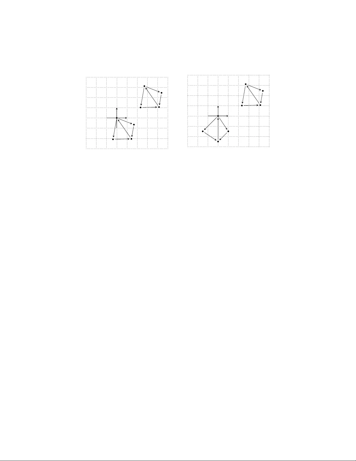
F ormation con trol P art I I: Algebraic asp ects of information ﬂo w and singularities M.-A. Belabbas ∗ Jan uary 14, 2011 Abstract Giv en an ensem ble of autonomous agen ts and a task to ac hiev e co operatively , ho w m uc h do the agen ts need to know about the state of the ensemble and about the task in order to achiev e it? W e introduce new metho ds to understand these aspects of decen tralized con trol. Precisely , we introduce a framework to capture what agen ts with partial information can ac hieve by co operating and illustrate its use b y deriving results about global stabilization of directed formations. This framework underscores the need to diﬀeren tiate the knowledge an agen t has about the task to accomplish from the knowledge an agen t has ab out the current state of the system. The con trol of directed formations has pro ven to be more diﬃcult than initially though t, as is exempliﬁed by the lac k of global result for formations with n ≥ 4 agents. W e established in part I that the space of planar formations has a non-trivial global top ology . W e propose here an extension of the notion of global stabilit y whic h, because it ackno wledges this non-trivial top ology , can b e applied to the study of formation con trol. W e then dev elop a framework that reduces the question of whether feedbac k with partial information can stabilize the system to whether tw o sets of functions in tersect. W e apply this framew ork to the study of a directed formation with n = 4 agents and show that the agents do not hav e enough information to implement lo cally stabilizing feedbac k laws. Additionally , w e sho w that feedbac k la ws that respect the information ﬂow cannot stabilize a target conﬁguration without stabilizing other, un w an ted conﬁgurations. Con ten ts 1 In tro duction 2 ∗ M.-A. Belabbas is with the School of Engineering and Applied Sciences, Harv ard Univ ersity , Cambridge, MA 02138 belabbas@seas.harvard.edu 1 2 Notions of stability 6 3 Singularities, genericit y and jet spaces 10 4 The Logistic equation 12 5 Algebraic aspects of distributed information 14 6 Lo cal stabilit y prop erties 19 6.1 Unstable equilibria . . . . . . . . . . . . . . . . . . . . . . . . . . . . . . . . 25 7 Singularities, transfer of stabilit y and the appearance of stable ancillary equilibria 30 7.1 Singular formations for n = 4 agents . . . . . . . . . . . . . . . . . . . . . . 30 7.2 T ransfer of stability or E s * E d . . . . . . . . . . . . . . . . . . . . . . . . . 31 8 Summary and conclusion 38 8.1 Summary . . . . . . . . . . . . . . . . . . . . . . . . . . . . . . . . . . . . . 38 8.2 Conclusion . . . . . . . . . . . . . . . . . . . . . . . . . . . . . . . . . . . . 39 9 Ac knowledgmen ts 40 A Example: u ( x ) = x 40 B Singularities of v ector ﬁelds, jet spaces and transv ersalit y 41 B.1 Jet Spaces . . . . . . . . . . . . . . . . . . . . . . . . . . . . . . . . . . . . . 42 C F actorization Lemma 44 D Proof of Theorem 3 46 1 In tro duction In Part I of this pap er, w e studied the geometry of the space of formations in the plane. In particular, w e established that the space of edge lengths-normalized formations of n agen ts is a complex pro jective space of dimension n − 2 and w e describ ed it explicitly for n = 3 and n = 4. This description relied on exhibiting discrete symmetry groups acting on frameworks and w e conjectured the existence of a relation b et ween these groups and Henneb erg sequences. By relating the conv exity of the space of edge lengths to a top ological c haracteristic of C P( n − 2), we also provided a low er b ound on the cardinalit y of the symmetry groups. In the last part, w e presen ted a general dynamical model for formation con trol that resp ected b oth the inv ariance of the system under rigid transformations of the 2 plane and the information ﬂow as describ ed by the underlying graph. Let us call this class of mo dels F . In this part, w e deﬁne tw o distinct global stabilit y prop erties of formation con trol and in vestigate them in the case of the 2-cycles formation. Namely , we know from P art I that there are 4 frameworks in the plane that corresp ond to a generic vector of edge lengths for the 2-cycles. W e answer the tw o following questions: “do es there exist a feedback system in F that makes these four frameworks locally stable?” and “do es there exist a control law that mak es an y of these four frameworks stable, and no other frameworks stable?” The ﬁrst question th us asks for the existence of a globally deﬁned con trol la w that will mak e the four formations corresp onding to a giv en edge lengths locally stable, whereas the second question is concerned with the existence of other stable formations. W e answ er these questions b y introducing new approac hes to analyze the space F . W e ﬁrst deﬁne an algebraic framework to c aptur e the r ange of b ehaviors that ar e r e alizable by elements of F . Lo osely sp eaking, the main idea behind our framework is the follo wing: w e associate to elemen ts of F a subset in the ring of smooth real-v alued functions on the state-space, and to the ob jectiv e that we w an t the decentralized con trol problem to ac hieve an ideal in that ring. W e then reduce the feasibilit y question to an intersection problem betw een these t w o spaces. Within this framework, questions suc h as ho w muc h more information should an agent hav e in order to achiev e an ob jectiv e tak e a particularly natural form. Indeed, we essentially reduce the problem of kno wing whether an ensemble of agents can accomplish a certain task to problems of the following t yp e: assume the task is enco ded in the zero set of a function p ( x + y ), and that the range of b ehaviors of the decen tralized system for this task is enco ded as the pro duct u 1 ( x ) u 2 ( y ). The feasibility of the ob jective is th us reduced to ﬁnding u 1 ( x ) and u 2 ( y ) smo oth and such that u 1 ( x ) u 2 ( y ) = 0 ⇔ p ( x + y ) = 0 , where it is understoo d here that agen t 1 observes x and agen t 2 observes y . If, for example, p is the identit y , then this is clearly p ossible if and only if u 1 or u 2 are identically zero. Hence, we conclude that w e would need to let agen t 1 or 2 access more information (e.g. let u 1 dep end on y ) in order to solve this problem in a non-trivial manner. W e revisit this example in Section 5, where these ideas are given a formal framew ork. An additional adv antage of this framework is that it allo ws the use of the many computational to ols that ha ve been developed, e.g. Gr¨ obner bases, to handle the algebraic structures in volv ed. The other metho d developed is the use of singularity theory to prov e the existence of ancillary equilibria in the dynamics of decentralized control systems. With the exception of some w ork on the relation b etw een Ly apunov theory and Morse theory [WY73], ideas from top ology and singularity theory hav e not play ed an imp ortant role in the analysis of globally stabilizing control la ws. In this pap er, we will sho w that such ideas can prov e to b e fundamental in understanding ho w well one can hop e to do in a control design task. In particular, w e will use ideas from singularit y theory [AAIS94, GSS88] to pro ve that if one 3 tries to stabilize a system at a giv en conﬁguration via a con tinuous feedbac k law, other equilibrium conﬁgurations app ear and are stable, th us prev enting global stabilit y . The 2-cycles formation (Figure 1b) is studied in depth in this pap er. Its imp ortance stems from its status as the second simplest problem in the class of directed formation problems, the simplest one b eing the triangular formation. This is a consequence of a theorem of Baillieul and Suri [BS03] that built upon earlier w ork of Bro ck ett [Bro83]. The result asserts that when the in teractions are asymmetric, or directed, one can generally require of an agent to hav e t wo leaders at the most. F rom this p oint of view, w e can understand the formation depicted in Figure 1b as b eing the formation right ab ov e the triangle in terms of complexit y . Indeed, this formation w as singled out in [CAM + 10] as the prototypical example of the diﬃcult y to make progress in this area and it underscored the need of new results to address decen tralized control problems. x 1 x 2 x 3 (a) x 1 x 2 x 3 x 4 (b) Figure 1: In Figure 1a, w e show three agents in a cyclic formation in the plane. Agen t 1 observ es agent 2, whic h observes agen t 3, which in turn observes agen t 1. In Figure 1b, w e depict the 2-cycles problem analyzed in detail in this paper. Agent 1 observ es agen ts 2 and 4, agen ts 2 and 4 observe agen t 3 which observes agen t 1. The results that are the closest to the formation con trol asp ect of this w ork rev olve around the triangle formation, lo cal stabilization prop erties and formation con trol with undirected information ﬂow. The triangular formation w as dealt with in a series of pap ers ([CAM + 10, CMY + 07] and references therein). More precisely , it was sho wn that there exists a control la w u which will satisfactorily stabilize triangular formations. F urthermore, a careful analysis exhibited a whole family of suc h laws and gav e a uniﬁed framework for the analysis of their conv ergence prop erties. In [Y ADF09], the lo cal stabilization of a given minimally p ersistent [HADB07] formation w as related to some easily chec k able condition in volving minors of a Jacobian. While the ﬁrst result is global, and carefully addresses the existence of a set of initial conditions that ma y result in the system evolving to an undesired conﬁguration, it do es not address formations with more than 3 agen ts. In contrast, the latter result handles formations of arbitrary size, but only addresses lo cal prop erties. F or similar work on the con trol of formations with symmetric in teractions, we refer the reader to [KBF08, SBF06]. 4 In order to put our results in p ersp ective, observe that the work of Y u, Anderson, Dasgupta and Fidan [Y ADF09] asserts that one can ﬁnd a lo cally stabilizing con trol law, via c ho osing appropriate feedbac k gains for the linearized system, for any giv en conﬁguration. The control laws w ere computed with complete kno wledge of the formation, thus separating the design stage from the dynamics stage. Our stability results state that, at least in the case of the t wo-cycles, these lo cal con trol laws c annot b e evaluate d by the agents with the information they have at their disp osal . Moreov er, we pro ve that such con trol laws in tro duce other stable equilibria. The pap er is organized as follows: in the second section, w e in tro duce a notion of global stability that is more appropriate to the study of decen tralized con trol problems. This notion of stability is w eaker than the usual one and ackno wledges some simple facts from Morse theory . In Section 3, we review the necessary bac kground in singularity theory , relegating the most tec hnical aspects of transv ersality and Thom’s theorem to an app endix. In Section 4, w e brieﬂy presen t the logistic equation. W e in tro duce in Section 5 an algebraic framew ork to capture the range of b eha viors of decen tralized con trol systems, and w e apply it in the following section by proving that one cannot make all framew orks corresp onding to a giv en edge length v ector stable. In Section 7, we prov e that feedbac k laws on the 2-cycles will generically make a stable ancillary equilibrium app ear. In the last section, w e discuss some forthcoming results and illustrate how a con trol la w that stabilizes the triangle formation fails to stabilize the 2-cycles. W e state the results that relate to the 2-cycles explicitly here: let x 1 , x 2 , x 3 , x 4 ∈ R 2 represen t the p ositions of the agen ts in the plane, and deﬁne z 1 = x 2 − x 1 , z 2 = x 3 − x 2 , z 3 = x 1 − x 3 , z 4 = x 3 − x 4 , z 5 = x 3 − x 1 . (1) Let e i = z i · z i − d i , where x · y is the inner pro duct of vectors x and y , b e the error b etw een the edge lengths and the target edge length d i . The ob jective of the formation control problem is to ﬁnd a control la w that drives the system to a conﬁguration with e i = 0 for i = 1 , . . . , 5. Consider the class of distributed feedbac k control systems, whic h resp ect the inv ariance under rigid transformations:        ˙ x 1 = u 1 z 1 + u 5 z 5 ˙ x 2 = u 2 z 2 ˙ x 3 = u 3 z 3 ˙ x 4 = u 4 z 4 (2) where u 1 and u 5 are smo oth functions of d 1 , d 5 , z 1 , z 5 and u i are smo oth functions of d i and z i for i = 2 , 3 , 4. W e will show that, for a set of p ositive measure of edge lengths, there 5 are no r obust distributed con trol laws that stabilize equilibria with edge lengths ( d 1 , ..., d 5 ), and moreov er, there will b e a stable equilibrium with e i 6 = 0. In other words, if there exists a u that accomplishes any of the tw o tasks ab o ve (i.e. stabilizing the four equilibria with e i = 0, or stabilizing at least one such equilibria while making sure no other formation is stable), then there is an r > 0 such that for all 0 < ε < r , and almost all ˜ u i , the system        ˙ x 1 = ( u 1 + ε ˜ u 1 ) z 1 + ( u 5 + ε ˜ u 5 ) z 5 ˙ x 2 = ( u 2 + ε ˜ u 2 ) z 2 ˙ x 3 = ( u 3 + ε ˜ u 3 ) z 3 ˙ x 4 = ( u 4 + ε ˜ u 4 ) z 4 (3) will fail to do b oth. Hence, the control law is not robust to the least error in mo delling or measuremen t. An imp ortant aspect is that w e need to only consider the set of p erturbations that r esp e ct the distribute d natur e of the con trol law. 2 Notions of stabilit y Consider the con trol system ˙ x = f ( x, u ( x )) (4) where x ∈ M , a smo oth manifold, and all functions are assumed smo oth. W e are mostly interested in glob al results ab out stabilization. F rom Part I, we kno w that formation con trol problems ev olv e on a manifold M with non-trivial homology groups [W ar83]. As a result of the Morse inequalities [Sma67], these systems cannot b e globally stable in the usual sense: there is no contin uous u suc h that (4) has a unique equilibrium. Such situations happ en frequen tly in nonlinear con trol, e.g. in steering con trol. Example 1. Contr ol pr oblems wher e one ne e ds to stabilize the dir e ction of motion of a vehicle ar e mo del le d by a dynamic al system evolving on the unit cir cle S 1 : ˙ x = f ( x ) , x ∈ S 1 . In this one-dimensional c ase, the Morse ine qualities r e duc e to the Poinc ar´ e-Hopf identity: X x = e quilibria ind x f ( x ) = χ ( S 1 ) , wher e χ ( M ) is the Euler char acteristic of M and ind x is the index of the ve ctor ﬁeld at the e quilibrium x . In the c ase of the cir cle, we c an pr ove that exp onential ly stable e quilibria c orr esp ond to e quilibria of index − 1 and, r e cipr o c al ly, exp onential ly unstable e quilibria to e quilibria of index 1 . Sinc e the Euler char acteristic of S 1 is χ ( S 1 ) = 0 , the Poinc ar´ e-Hopf identity b e c omes: # exp onential ly stable e quil. = # exp onential ly unstable e quilibria . 6 1 − 1 − 1 1 − 1 1 Figure 2: W e represent three con tinuous v ector ﬁelds on the circle. The one on the left has no equilibrium, the one in the center has one stable equilibrium and one unstable equilibrium and the one on the righ t has tw o stable equilibria and t wo unstable equilibria; the indices of the equilibria are indicated on the Figure. Because the sum of the indices is constrained to be zero, there is an ev en n umber of equilibria and, in particular, no con tinuous system on the circle can be globally stable. We il lustr ate it in Figur e 2. F or every stable e quilibrium, the top olo gy of S 1 thus for c es the app e ar anc e of an unstable e quilibrium. Henc e, system evolving on S 1 c annot b e glob al ly stable in the usual sense. F rom a practical p oin t of view, ho w ev er, if one could mak e one equilibrium stable, and all other equilibria either saddles or unstable, the system would b ehav e as if it were globally stable. Indeed, a v anishingly small p erturbation would ensure that the system, if at a saddle or unstable equilibrium, evolv es to the unique stable equilibrium. W e formalize and elab orate on this observ ation here. Let E d b e a ﬁnite subset of M con taining conﬁgurations that w e w ould lik e to stabilize via feedback. All conﬁgurations in E d are equally appropriate for the stabilization purp ose. W e are thus in tereste d in the design of a smo oth feedbac k control u ( x ) that will stabilize the system to an y p oint x 0 ∈ E d . W e call these p oints the design tar gets or design e quilibria : E d = { x 0 ∈ M s.t. x 0 is a design equilibrium } Let E = { x 0 ∈ M s.t. f ( x 0 , u ( x 0 )) = 0 } , the set of equilibria of (4). W e assume that E is ﬁnite. As explained ab ov e, when the system evolv es on a non-trivial manifold, the Morse inequalities make it unreasonable to exp ect that there exists a con trol u ( x ) that makes the design equilibria the only equilibria of the system, i.e. suc h that E d = E . W e call these additional equilibria, that are introduced by the non-trivial top ology of the space, ancil lary e quilibria : E a = E − E d . 7 Example 2. In the c ase of the 2-cycles pr oblem, ther e ar e ﬁve distanc e c onstr aints to satisfy. As was shown in Part I, four formations in the plane, mo dulo r otation and tr ans- lation, satisfy the distanc e c onstr aints; henc e, |E d | = 4 . Given d ∈ L , we c al l framew orks attac hed to d the fr ameworks whose e dge lengths ar e given by d . Equivalently, fr ameworks attache d to d ar e given by letting the r eﬂe ctions R 1 and R 2 deﬁne d in Se ction 4 or p art I act on any fr amework with e dge lengths d . We il lustr ate these fr ameworks in Figur e 3. Notic e that the mirr or-symmetric of a formation c annot b e obtaine d via r otations and tr anslations. x 1 x 2 x 3 x 4 (a) x 1 x 2 x 3 x 4 (b) x 1 x 2 x 3 x 4 (c) x 1 x 2 x 3 x 4 (d) Figure 3: F our formations in the plane that are not equiv alent under rotations and trans- lation and that hav e the same corresp onding edge lengths. ( a ) is the mirror-symmetric of ( c ) and ( b ) is the mirror-symmetric of ( d ). Let us assume for the time being that the linearization of the system at an equilibrium has no eigenv alues with zero real part. W e decomp ose the set E into stable equilibria, b y which w e mean equilibria such that al l the eigenvalues of the linearized system hav e a negativ e real part, and unstable e quilibria , where at le ast one eigenvalue of the linearization has a p ositiv e real part. Observ e that under this deﬁnition, saddle points are considered unstable; this is motiv ated b y practical considerations since the set of initial conditions that result in a system settling at a saddle p oin t is of measure zero 1 . Equiv alen tly , p erturbations will mo ve the system aw ay from the α − set [GH83] of a saddle point with probability one. In summary: E = E s ∪ E u 1 for e.g. the Lebesgue measure on M 8 where E s = { x 0 ∈ E | x 0 is stable } and E u = { x 0 ∈ E | x 0 is unstable or a saddle } . With these notions in mind, w e introduce the following deﬁnition: Deﬁnition 1. Consider the smo oth c ontr ol system ˙ x = f ( x, u ( x )) wher e x ∈ M and the set E of e quilibria of the system is ﬁnite. L et E d ⊂ M b e a ﬁnite set. We say that E d is 1. feasible if we c an cho ose a smo oth u ( x ) such that E d ∩ E 6 = ∅ . 2. t yp e-A stable if we c an cho ose a smo oth u ( x ) such that E s ⊂ E d . 3. strongly t yp e-A stable if we c an cho ose a smo oth u ( x ) such that E s = E d . When the set E d is cle ar fr om the c ontext, we say that the system is typ e-A stable. The set E d is feasible if we can choose u ( x ) such that at le ast one equilibrium of the system is a design target. It is said to b e typ e-A stable if the system stabilizes to E d with probabilit y one for an y randomly chosen initial conditions on M . It is str ongly typ e-A stable if it is t yp e-A stable and moreo ver all elemen ts of E d are stable equilibria. The usual notion of global stability is a particular instance of type-A stabilit y; indeed, it corresp onds to having u ( x ) suc h that E d = E = E s . Lo oking at the contrapositive of this deﬁnition, a system is not typ e-A stable if there exists a set of initial conditions, which is of strictly p ositive measure, that lead to an ancillary equilibrium. W e observe that type-A stabilit y is a global stability notion; in particular, if one can choose u such that all design equilibria are lo cally stable, but if this c hoice forces the app earance of other, undesired equilibria whic h are also lo cally stable, the system is not t yp e-A stable. The examples b elo w illustrate these notions. Example 3. Consider a system ˙ x = x (1 − k x 2 ) wher e k ∈ R is a fe e db ack p ar ameter to b e chosen by the user. We show that any E d ⊂ (0 , ∞ ) is not typ e-A stable. We ﬁrst observe that the system has an e quilibrium at 0 and two e quilibria at x = ± p 1 /k if k > 0 . The system is thus fe asible for any E d ⊂ R . The Jac obian of the system is 1 at x = 0 and − 2 at x = ± p 1 /k . F or k > 0 , the ab ove says that E = { 0 , ± p 1 /k } = { p 1 /k } | {z } E d ∪ { 0 , − p 1 /k } | {z } E a . 9 x f ( x ) f ( x ) Figure 4: The set E s is the set of lo cal minima (marked b y × ); the set E u is the set of saddles and lo cal maxima (mark ed b y · ). A gradien t ﬂow is type-A stable if and only if E d con tains the set of lo cal minima. F r om the line arization of the system, we have that E s = {± p 1 /k } and E u = { 0 } . We c onclude that E s * E d and the system is not typ e-A stable. Example 4 (Gradien t ﬂows) . L et f ( x ) : R n → R b e a smo oth function. Assume that a c ontr ol system is given by the gr adient ﬂow of f : ˙ x = − ∂ f ∂ x . We have that E s is the set of lo c al minima of f and E u c ontains al l the other p oints x 0 such that ∂ f ∂ x | x 0 = 0 . Henc e, E d is typ e-A stable if and only if it c ontains the set of lo c al minima of the gr adient ﬂow. We il lustr ate this in Figur e 4. 3 Singularities, genericit y and jet spaces Informally sp eaking, a prop erty of elements of an arbitrary set is said to b e generic if it is shared b y almost al l elements of the set. The set in question could b e a manifold if one is considering all possible initial conditions of a Cauch y problem, or C 2 ( M ) if one is considering the class of twice-diﬀeren tiable functions on M . Precisely , we ha ve the deﬁnition: 10 Deﬁnition 2. A pr op erty P is generic for a top olo gic al sp ac e S if it is true on an everywher e dense interse ction of op en sets of S . Ev erywhere dense in tersections of op en sets are sometimes called r esidual sets [AAIS94]. In general, asking for a given prop erty to b e generic is a rather strong requiremen t, and often times it is enough to show that a given prop erty is true on an op en set of parameters, initial conditions, etc. W e deﬁne Deﬁnition 3. An element u of a top olo gic al sp ac e S satisﬁes the pr op erty P robustly if P is true in a neighb orho o d of u in S . If the prop erty is satisﬁed for a non-r obust u , then it fails to b e satisﬁed under the sligh test error in mo delling or measuremen t. W e also say that a pr op erty is r obust to refer to the existence of a robust u whic h satisﬁes the prop ert y . Remark 1. We emphasize that when we se ek a r obust c ontr ol law u ( x ) for stabilization, we se ek a c ontr ol law such that the e quilibrium r emains stable under smal l p erturb ations in u ( x ) . The e quilibrium, however, may move in the state sp ac e. F or example, assume that the system ˙ x = u ( x ) has the origin as a stable e quilibrium. If for al l g ( x ) in an appr opriate set of p erturb ations, the system ˙ x = u ( x ) + εg ( x ) has a stable e quilibrium at a p oint k ( ε ) ne ar the origin, then the c ontr ol law u ( x ) is r obust. If, on the c ontr ary, the e quilibrium disapp e ars or b e c omes unstable, then u ( x ) is not r obust. Genericit y will app ear in tw o guises in this work. The ﬁrst app earance was in the previous section: w e can paraphrase the deﬁnition of type-A stability b y saying that a system is type-A stable if it will ev olve to the set E d generic al ly with resp ect to the c hoice of initial conditions. The other is the sub ject of this section: we will restrict our searc h to r obust c ontr ol laws u ( x ) for a prop erty P , where P is either type-A stability or strong t yp e-A stabilit y . If eP , the opp osite of P , is generic, then there is no robust u that satisﬁes P . Indeed, if eP is generic, then P is v eriﬁed on at most a nowhere dense closed set. In particular, P is not veriﬁed on an op en set. W e present the main to ols to handle genericity and robustness in App endix B. 11 4 The Logistic equation W e now recall a few deﬁnitions from dynamical systems theory . Consider a dynamical system of the form ˙ x = f µ ( x ) (5) where x ∈ M , an n − dimensional manifold, and µ ∈ R k is a vector of parameters on which the system smo othly dep ends. Deﬁnition 4 (Hyp erb olic equilibrium and bifurcation v alue) . 1. An e quilibrium x 0 is c al le d hyperb olic if the eigenvalues of the line arization at x 0 have non-zer o r e al-p arts. 2. A value µ 0 in the p ar ameter sp ac e R k for which the ﬂow of (5) has an eigenvalue with zer o r e al-p art is c al le d a bifurcation v alue . Let us put the deﬁnition abov e in con text. Assume that x 0 is an equilibrium. If it is h y- p erb olic, the dynamics in a neighborho o d of x 0 is determined b y the num b er of p ositive and negativ e eigen v alues of ∂ f ∂ x | x 0 . Precisely , the Hartman-Grobman theorem [Gro59, Har60] asserts the existence of a homeomorphism that takes the ﬂow in a neighborho o d of x 0 to the ﬂo w of ˙ z =  I l 0 0 − I m  z where I l is the l × l identit y matrix and l , m are the num b er of p ositive and negative eigen v alues of ∂ f ∂ x | x 0 , resp ectively . The image of [ z 1 , . . . , z l ] T under the homeomorphism is called the unstable manifold, and the image of [ z l +1 , . . . , z l + k ] T the stable manifold. Hence, under the assumption that an equilibrium is hyperb olic, the b ehavior of the system in a neigh b orho o d of that equilibrium is en tirely determined b y its linearization. A t least since the w ork of Andronov and P on tryagin [AP37], it has b een recognized that the b ehavior of systems around bifurcation p oints can be far more complex than the usual stable/unstable manifolds decomp osition of h yp erb olic dynamics [GH83]. As examples of the wide v ariet y of situations can o ccur nearb y a bifurcation v alue, w e mention that p erio dic orbits may app ear (e.g. in the Andronov-Hopf bifurcation) or the dimensions of the stable and unstable manifolds ma y change (e.g. the transcritical bifurcation). In general, suc h singularities of v ector ﬁelds are not generic since a small p erturbation of f will make its Jacobian non-singular (see Corollary 2 b elow). W e will see though that the distribute d natur e of the system makes the existenc e of such singularities generic . W e come bac k to this p oin t in Section 8. W e show b elo w that the 2-cycles b ehav es similarly to the logistic equation, whic h is presented here, in the sense that they b oth exhibit the same t yp e of singularities or bifurcation. The logistic equation, which is often used to describ e systems in which t wo 12 stable µ Equilibria unstable 0 Figure 5: The logistic equation undergoes a transcritical bifurcation when µ = 0. The equilibrium x = 0 is stable for µ < 0 and unstable for µ > 0. comp eting eﬀects—such as supply and demand or predator and prey— are at pla y , is the one-dimensional ODE giv en by ˙ x = x ( µ − x ) . (6) This equation displays what is called a tr anscritic al or tr ansfer of stability bifurcation at µ = 0, which we explain here. Observe that it has tw o equilibria, one at x = 0 and one at x = µ , which coalesce when µ = 0. The linearization of the system ab out x is d f = ( µ − x ) − x = µ − 2 x. F rom this linearization, we see that for µ > 0, the equilibrium x = 0 is unstable whereas the equilibrium x = µ is stable. The situation is rev ersed for µ < 0. W e conclude that at the bifurcation v alue µ = 0, the tw o equilibria coalesce and exchange their stability pr op erties . W e depict the ab ov e in Figure 5. This ﬁgure is to b e compared to Figure 14. The most common approac h used to gain some understanding ab out the b eha vior of a dynamical system near a non-h yp erb olic equilibrium relies on the use of the c enter manifold the or em [GH83]. This theorem asserts the existence of a nonlinear change of co ordinates, v alid near the equilibrium, where the dynamics can b e put in a so-called normal form whic h is more amenable to analysis. While very useful in general, such an approac h is without m uch hope for success for our ob jective. Indeed, the c hange of v ariables inv olv ed in the analysis will dep end on the control u , and tracking the eﬀect of this dependence through the whole pro cedure is not feasible for broad classes of control la ws. Sp eciﬁcally , in order to sho w that the 2-cycles b ehav es similarly to the logistic equation generically for u using a cen ter manifold approac h, one w ould ha v e to exhibit a u -dep endent nonlinear change of co ordinates near singular formations that reduces the 2-cycles to the normal form (6). In order to sidestep this diﬃcult y , w e hav e recourse to the follo wing result of So- toma yor [Sot73], which characterizes the generic b eha vior of dynamical systems near non- 13 h yp erb olic ﬁxed-p oin ts without r e c ourse to the cen ter manifold. Theorem 1 (Sotomay or) . L et ˙ x = f µ ( x ) b e a system of ODE in R n dep ending on a sc alar p ar ameter µ . F or µ = µ 0 , assume that the system has an e quilibrium x 0 satisfying the fol lowing c onditions: 1. ∂ f µ 0 ∂ x | x 0 has a unique zer o eigenvalue with left and right eigenve ctors w and v r esp e c- tively. The other eigenvalues ar e ne gative. 2. w T ∂ f µ ∂ µ | x 0 ,µ 0 v = 0 3. w T ∂ 2 f µ 0 ∂ x 2 | x 0 ( v , v ) 6 = 0 and w T ∂ 2 f µ ∂ x∂ µ | x 0 ,µ 0 ( v , v ) 6 = 0 Then the phase p ortr ait is top olo gic al ly e quivalent to the phase p ortr ait of the lo gistic e qua- tion, i.e. we have a tr anscritic al bifur c ation ab out x 0 for µ = µ 0 . Thus ar ound µ = µ 0 , ther e ar e two ar cs of e quilibria whose stability pr op erties ar e exchange d when p assing thr ough µ 0 . Mor e over, the set of e quations ˙ x = f µ ( x ) which satisfy c onditions (1) , (2) and (3) ab ove is generic in the sp ac e of smo oth one-p ar ameter families of ve ctor ﬁelds with an e quilibrium at x 0 , µ 0 with a zer o eigenvalue. W e will use this theorem to show that the 2-cycles admits a transcritical bifurcation generically and that, as a consequence, E s * E d . 5 Algebraic asp ects of distributed information W e establish in this section an algebraic framework that reduces questions in decen tral- ized con trol problems to algebraic ones. Informally sp eaking, w e capture in an algebraic ob ject the range of b ehaviors that can b e achiev ed giv en the information ﬂow of a decen- tralized system. W e illustrate this approac h in the next section to show that the 2-cycles is generically not strongly t yp e-A stable. Consider a general decen tralized feedback system of the t yp e  ˙ x = P i u i ( y i ) g i ( x ) = G u ( x ) y i = h i ( x ) (7) where the g i ( x ) are smo oth v ector ﬁelds, and the u i are smo oth real-v alued functions that b elong to a set U of admissible control laws. The h i ( x ) are the observ ations on the system. What makes the system de c entr alize d is the fact that through h i , each con trol term u i only has access to partial information about the system. The h i ’s deﬁne an information ﬂow together with the u i ’s. In the case of formation con trol problems, w e ha ve h i ( x ) = k x k 2 − d i or h i ( x ) = ( e j , e k , ( x k − x i ) · ( x j − x i )) dep ending on the num b er of co-leaders of the agen t. Giv en a decentralized control system and an ob jective to attain, there are tw o notions that need to b e formalized in order to kno w if the ob jective is feasible: 14 - What is the range of b ehaviors that can b e achiev ed by letting u ∈ U ? - What are the diﬀeren t w a ys to achiev e the ob jective? The ﬁrst notion calls for the description of a reac hable set in the space of vector ﬁelds, or said diﬀerently , a c haracterization of the p ossible right-hand sides of Equation (7). The second notion, on whic h we elaborate b elow, ackno wledges the fact that there often is a class of system whic h satisfy an ob jectiv e. The class is sometimes explicitly given, e.g. when asking for control la ws that will mak e some eigen v alues negative, or it can be implicitly giv en, e.g. when requiring that a function v anishes at a p oint without specifying the order with whic h it should v anish. W e propose a framework that addresses these tw o aspects in an algebraic manner. Since the work of Riemann, it has b een recognized that there is a duality to b e exploited b et w een top ological spaces and functions on these spaces. This change of p oin t of view— replacing the study of a space M b y the study of functions on that space—has prov en remark ably fruitful. Indeed, it has b ecome standard in algebraic geometry , where a v ariety is studied through sheav es of regular functions, and it is at the core of noncommutativ e geometry , where the top ological space is all but replaced by a noncommutativ e algebra of functions. This point of view is b est summarized b y a consequence of the celebrated Gelfand-Neimark theorem asserting that if M is compact and Hausdorﬀ, w e can recov er M from the knowledge of the ring of smo oth complex-v alued functions on M . As a consequence, the study of all control problems on M could b e reduced, at least in principle, to the study of algebraic ob jects in spaces of functions on M . This approach w ould rely on translating the v ector ﬁeld/diﬀerential description of the system and the ob jective to a functional description. While this may not bring muc h to general con trol systems, w e b elieve it can b e v ery fruitful to answer questions ab out decen tralized con trol systems. W e dev elop suc h an approach here. Precisely , we propose a framework that yields algebraic equiv alents to the tw o notions ab ov e and reduce the feasibility of an ob jective to an in tersection condition. W e start b y reviewing some notions from algebra. A ring R is a set with t wo op er- ations, addition and m ultiplication, whic h hav e the following prop erties: R is an ab elian group for the addition (i.e. the addition is comm utative, asso ciative, and there is an ad- ditiv e inv erse for ev ery element); the multiplication op eration is asso ciativ e and it has an iden tity elemen t, but no in verses in general. Moreov er, the m ultiplication and addition op erations are distributive. W e will work here mostly with the commutativ e ring C ∞ ( M ) of smo oth real-v alued functions on a manifold M where addition and multiplication are tak en p oin twise. Let us illustrate the ab o v e p oin t of view on a simple example. Consider the scalar system    ˙ x = f ( x ) + k ( x ) u ( y ) = g ( x ) y = x 2 u ∈ U . 15 Consider the space of functions h g ( x ) i U =  g ( x ) ∈ C ∞ ( R ) s.t. g ( x ) = f ( x ) + k ( x ) u ( x 2 ) for some u ∈ U  . This space of functions enco des all the p ossible b ehaviors of the system. F or example, let p ( x ) b e a smo oth function such that p ( x 0 ) = 0. If p ( x ) ∈ h g ( x ) i U , then there exists a feedbac k such that x 0 is an equilibrium for the system. The diﬀerent w a ys in which feedbac k can create an equilibrium at x 0 is reﬂected in the diﬀeren t functions in h g ( x ) i U that v anish at x 0 . W e formalize this as follows: recall that an ide al I in a ring R is a subset of R that is closed under addition and has the prop ert y that f ∈ R and h ∈ I ⇒ f h ∈ I . Consider the ideal I ( x 0 ) of functions that v anish at x 0 . In general, given a subspace C ⊂ M , w e deﬁne the ideal of functions that v anish on C : I ( C ) = { g ∈ C ∞ ( M ) such that g ( x ) = 0 for all x ∈ C. } This is indeed an ideal since g ∈ I ( C ) implies f ( x ) g ( x ) = 0 for all x ∈ C, f ∈ C ∞ ( M ) and I ( C ) is closed under addition. A necessary and suﬃcient condition for the existence of a feedbac k such that x 0 is an equilibrium is th us given b y h g i U ∩ I ( x 0 ) 6 = ∅ . The ab ov e condition eﬀectively replaces the scalar equation f ( x ) + k ( x ) u ( x 2 ) = 0: we have thus substitute d to a sc alar e quation in unknown u a pr oblem involving the interse ction of function sp ac es with ide als. Beyond the fact that an algebraic approach lends itself to concise statemen ts for feasibility , another adv antage of translating the problem into algebraic terms is that ther e exist wel l-develop e d metho ds to che ck whether an element b elongs to an ide al for many classes of functions. In case the problem is restricted to analytic control systems, there exists a large b o dy of literature on computational metho ds to handle the ob jects deﬁned ab ov e (e.g. Gr¨ obner Bases) [Sch03]. Our approac h is, in broad strokes, the follo wing: 1. Enco de the task of the decentralized control problem as a prop er ideal in the ring of smo oth functions C ∞ ( M ). Call this ideal I . 2. Enco de the range of b ehaviors, with r esp e ct to the task at hand , that the system can ac hieve via feedbac k con trols u depending on the information ﬂo w as a set of functions h F i U . 3. Conclude that a necessary condition for the existence of u ’s that achiev e the task is that h F i U ∩ I 6 = ∅ . 16 W e derive now a simple necessary criterion for feasibilit y that will b e used in the next section. Let F ∈ C ∞ b e with the conv ention that F ( x ) ≥ 0 is a necessary condition for the ob jective to b e met. W e sa y that F is fe asible if w e can c ho ose u ’s such that F ( x ) ≥ 0. The situation w e ha v e in mind is the one of stabilit y , where we take F i ( x ) to b e minus the i th eigen v alue of the linearization at an equilibrium x . Hence, F i ( x ) ≥ 0 is a necessary condition for stabilit y . Assume that at an equilibrium x , w e hav e F ( x ) = p ( x ) q ( x ) (8) where q ( x ) dep ends on the u ’s and p ( x ) is indep enden t of u . W e deﬁne by V ( p ) the zero set of p ( x ), i.e. V ( p ) = { x ∈ M s.t. p ( x ) = 0 } Th us I ( V ( p )) is the ideal in C ∞ ( M ) of functions that v anish where p v anishes. Informally sp eaking, a function p ( x ) is transv ersal to a submanifold C of M if the columns of ∂ ∂ x p ( x ) and a basis for the tangen t space of C spans the tangen t space of M . F or example, the function y = x 2 is not transversal to the submanifold y = 0 of R 2 at 0, but the function y = x is. F or a formal deﬁnition, see Deﬁnition 6 in App endix B. W e hav e the follo wing result: Lemma 1. Assume that we c an factor F ( x ) as F ( x ) = p ( x ) q ( x ) with p indep endent of u . L et p ( x ) by such that V ( p ) is of c o dimension 1. If p ( x ) is tr ansversal to V ( p ) , then F ≥ 0 is fe asible only if h q i U ∩ I ( V ( p )) 6 = ∅ . Pr o of. Because p ( x ) is transv ersal to V ( p ) at x and V ( p ) is of co dimension 1, p ( x ) changes sign around x . In order for F ( x ) to remain positive, q ( x ) needs to v anish at x and thus b elong to I ( V ( p )).  Recall that a function is regular at x 0 if its Jacobian is of full rank at x 0 ; x 0 is also called a regular point for h . Let h : M → R k where M is of dimension n > k . By the implicit function theorem, the set deﬁned by h ( x ) = h ( x 0 ) has the structure of a manifold in a neigb orho o d V x 0 of x 0 . W e call this manifold N h ( x 0 ): N h ( x 0 ) = { x ∈ V x 0 ⊂ M s.t h ( x ) = h ( x 0 ) } . (9) Lemma 2. L et C b e a smo oth submanifold of dimension m in an n-dimensional manifold M . L et h ( x ) : M → R k and u ( y ) : R k → R b e smo oth functions such that u ( h ( x )) ∈ I ( C ) . 17 N h ( x 0 ) U C C x 0 Figure 6: The submanifold N h ( x 0 ) (the isolevel set of h at the v alue h ( x 0 )) and C intersect transv ersally at x 0 . The dotted curv es represen t N h ( c ) for c in a neigh b orho o d U ⊂ C of x 0 . Because u ( h ( c )) v anishes on U and b ecause the v alue of u ( h ( x )) is constant on all N h ( c ) b y construction, u ( h ( c )) v anishes on an op en neighborho o d of x 0 in M . L et x 0 ∈ C b e a r e gular value for h . If N h ( x 0 ) interse cts C tr ansversal ly at x 0 , then u ( h ( x )) is zer o on an op en set in M and u ( y ) is zer o on an op en set in R k . In p articular, if we r estrict u to b e analytic, then u ≡ 0 .. Pr o of. The proof is straigh tforward; in the interest of space, we only sk etch it. Without loss of generalit y , w e can take M = R n , x 0 = 0, h ( x 0 ) = 0, C = R m and N h (0) = R n − k . Assume ﬁrst that C and N h (0) in tersect only at 0: C ∩ N h (0) = { 0 } ; b ecause they intersect transversally , we hav e that m = n − k . Let U b e a neighborho o d of 0 in C and let c ∈ U . Because 0 is a regular v alue of h , a neighborho o d of 0 in M is con tained in ∪ c ∈ U N h ( c ). Since u ( h ( x )) ∈ I ( C ) and c ∈ U , then u ( h ( c )) = 0 for c ∈ U . By deﬁnition of N h , for all x ∈ N h ( c ), w e ha ve h ( x ) = h ( c ) and thus u ( h ( x )) v anishes on ∪ c ∈ U N h ( c ) whic h prov es the ﬁrst part. F or the second part, since 0 is a regular v alue of h , h ( x ) maps a neighborho o d of zero in R m on to a neigh b orho o d V of 0 in R k . The previous p oin t thus implies that u v anishes on V . In case C and N h in tersect on a subspace of strictly p ositive dimension, the argumen t is the same as the one ab ov e but applied to a space C 0 that is contained in C but whose in tersection with N h is { 0 } . W e omit the details. The last part uses the fact that the only analytic function that v anishes on an op en set is the constant 0.  This lemma is useful to pro ve that there are no robust elemen ts in an ideal of functions. Indeed, if its conditions are met, by Corollary 2, u ( x ) is not robust since it v anishes with 18 a zero deriv ative. The proof that the 2-cycles formation is not robustly strongly t yp e-A stable relies on the same idea as the one dev elop ed in the example b elo w, alb eit applied to a more complex ideal. Example 5. L et f ( x, y ) = u 1 ( x ) u 2 ( y ) and C 1 b e the subsp ac e of R 2 deﬁne d by the e quation x − y = 0 . Ther e ar e no r obust choic es of u 1 and u 2 such that f ( x, y ) ∈ I ( C ) . Pr o of. Let h 1 ( x, y ) = x and h 2 ( x, y ) = y . Since the Jacobians of h 1 and h 2 are alwa ys of full rank, ev ery p oint in R 2 is a regular v alue for h 1 and h 2 . Because all the functions in volv ed are contin uous, if f is to v anish everywhere on C , there exists a connected op en set V in C suc h that either u 1 ( h 1 ( x, y )) or u 2 ( h 2 ( x, y )) v anishes. Assume without loss of generalit y that u 1 ( h 1 ( x )) ∈ I ( V ) and let x 0 ∈ V . The isolevel sets of h 1 are translations of the y-axis in R 2 , hence N h 1 in tersects C transversally ev erywhere. F rom Lemma 2, we deduce that u 1 is zero in an op en set in R and hence b y Corollary 2, it is not robust.  W e conclude this section by recording a few simple prop erties of the op erations V and I that we will use in the sequel. W e refer the reader to [Sch03] for more details. Assume that p 1 and p 2 , smo oth functions on M , are such that V ( p 1 ) ⊂ V ( p 2 ) ⇒ ( V ( p 2 )) ⊂ I ( V ( p 1 )) . (10) Moreo ver, observ e that V ( p 1 p 2 ) = V ( p 1 ) ∪ V ( p 2 ) (11) since the pro duct p 1 ( x ) p 2 ( x ) of course v anishes if and only if p 1 ( x ) or p 2 ( x ) v anish. Simi- larly , I ( V ( p 1 ) ∪ V ( p 2 )) = I ( V ( p 1 )) ∩ I ( V ( p 2 )) . (12) 6 Lo cal stabilit y prop erties W e show that the 2-cycles formation is not robustly strongly t yp e-A stabilizable or, equiv- alen tly , that there do es not exist robust feedbac k la ws that will stabilize its four design equilibria. W e established in part I a few conditions a feedback con trol law had to satisfy in order to yield a well-deﬁned formation con trol system (Deﬁnition 7 in part I). W e recall them here: Deﬁnition 7, part I: A fe e db ack c ontr ol law u i is compatible with a formation c ontr ol pr oblem if 1. u i ( d j ; e j ) is such that u i ( d j ; 0) = 0 if agent i has one c o-le ader. 2. u i ( d j , d k ; e j , e k , z j · z k ) is such that u i ( d j , d k ; 0 , 0 , z ) = 0 for al l z if agent i has two c o-le aders. 19 W e accordingly deﬁne the class of controls U to b e all smo oth con trol laws such that u i ( d i ; e i ) = 0 and u j ( d i , d j ; e i , e j , · ) = 0 for e i = e j = 0, dep ending on whether the agen t has one or t wo co-leaders. Let x i ∈ R 2 , i = 1 . . . 4 represen t the p ositions of the agents. Recall the deﬁnition of the v ectors            z 1 = x 2 − x 1 z 2 = x 3 − x 2 z 3 = x 1 − x 3 z 4 = x 3 − x 4 z 5 = x 4 − x 1 (13) Let d = ( √ d 1 , . . . , √ d 5 ) ∈ L be a target edge length. W e use the square ro ots in order to ha ve d i en ter the expression of the error in edge lengths linearly: e i = z i · z i − d i . The e i are lo wer-bounded b y the d i but not upp er-b ounded. W e deﬁne the set of vector ﬁelds F to b e the set of admissible v ector ﬁelds for the 2-cycles formation: F =            ˙ z 1 = u 2 ( d 2 ; e 2 ) z 2 − u 1 ( d 1 , d 5 ; e 1 , e 5 , z 1 · z 5 ) z 1 − u 5 ( d 1 , d 5 ; e 5 , e 1 , z 1 · z 5 ) z 5 ˙ z 2 = u 3 ( d 3 ; e 3 ) z 3 − u 2 ( d 2 ; e 2 ) z 2 ˙ z 3 = u 1 ( d 1 , d 5 ; e 1 , e 5 , z 1 · z 5 ) z 1 + u 5 ( d 1 , d 5 ; e 5 , e 1 , z 1 · z 5 ) z 5 − u 3 ( d 3 ; e 3 ) z 3 ˙ z 4 = u 3 ( d 3 ; e 3 ) z 3 − u 4 ( d 4 ; e 4 ) z 4 ˙ z 5 = u 4 ( d 4 ; e 4 ) z 4 − u 1 ( d 1 , d 5 e 1 , e 5 , z 1 · z 5 ) z 1 − u 5 ( d 1 , d 5 ; e 5 , e 1 , z 1 · z 5 ) z 5 , u i ∈ U            (14) There are four design equilibria for a generic d ∈ L (see Figure 3). They are suc h that e i = 0. W e pro ve the follo wing: Theorem 2. Ther e is a set of p ositive me asur e in L for which the 2-cycles formation is not r obustly str ongly typ e-A stable. Precisely , w e prov e the existence of a set of d ’s, of strictly p ositiv e measure in L , whic h share the characteristic that at least one of their four design equilibria is unstable for robust u i in Equation (14). It has recently b een prov ed [Y ADF09] that the 2-cycles can b e lo cally stabilized at a giv en framework in the plane using a relatively simple control law and adjusting some feedbac k gains. The dynamics used w as of the t yp e of Equation 14 with the control la w u i = k i e i , i = 1 , . . . , 5 20 where the k i are real-v alued gains used b y the agents to stabilize a given framew ork. It is not guaran teed that such control laws b ehav e well when the system is not near the equilibrium for whic h the gains ha ve b een designed. Theorem 2 states, in contrast, that there are no glob al ly deﬁne d decentralized feedbac k la w that stabilizes al l design equilibria lo cally . A ma jor diﬀerence b etw een the tw o approac hes is that the gains in [Y ADF09] are computed using the c omplete know le dge of the fr amework whereas w e will consider here all p ossible feedbac k gains that r esp e ct the de c entr alize d natur e of the system . Our result th us sho ws that the feedback laws of [Y ADF09] cannot b e computed in a decen tralized manner b y the agents. W e use for the remainder of this section the following parametrization of E 4 , the space of planar framew orks with 4 agen ts: a formation is represented by ¯ x = [ ¯ x 2 , ¯ x 3 , ¯ x 4 ] where ¯ x i is obtained b y translating the formation in order to hav e x 1 at the origin: ¯ x 2 = x 2 − x 1 ; ¯ x 3 = x 3 − x 1 ; ¯ x 4 = x 4 − x 1 ; similarly ¯ z 1 = ¯ x 2 − ¯ x 1 = ¯ x 2 , etc. W e also use ¯ x to diﬀerentiate these co ordinates from the dynamical co ordinates x : ¯ x describes an equilibrium or target for the system whereas x ( t ) represen ts the p osition of the system at time t . With the notation of the previous section, the functions h 1 ( ¯ x, x ) = ( d 1 , d 5 , z 1 · z 5 ) , h 2 ( ¯ x ) = d 2 , h 3 ( ¯ x ) = d 3 , h 4 ( ¯ x ) = d 4 enco de the information that is a v ailable to agents 1 to 4 resp ectively at an e quilibrium to compute gains. Informally sp eaking, the e i v ariables are of no help at design equilibria since they alw ays satisfy e i = 0; they are th us omitted in the h i ’s. W e call lo c al gains of agen ts 2 , 3 and 4 the functions u 2 x ( h 2 ; 0) = ∂ ∂ x u 2 ( d 2 ; x ) | x =0 , u 3 x ( h 3 ; 0) and u 4 x ( h 4 ; 0). Agent 1 has access to more information and has thus four lo cal gains u 1 x ( h 1 ( x )) = ∂ ∂ x u 1 ( d 1 , d 5 ; x, y , z 1 · z 5 ) | x,y =0 , u 1 y ( h 1 ( x )), u 5 x ( h 1 ( x )), u 5 y ( h 1 ( x )) and u 5 y ( h 1 ( x )). The solution pro vided in [Y ADF09] corresp onds to letting each lo cal gain dep end on h ( ¯ x ) = ¯ x. W e use the notation k i ( d i ) = u ix ( h i ; 0) for i = 2 , 3 , 4 k 11 ( d 1 , d 5 , z 1 · z 5 ) = u 1 x ( h 1 ( ¯ x, x )) k 12 ( d 1 , d 5 , z 1 · z 5 ) = u 1 y ( h 1 ( ¯ x, x )) k 51 ( d 1 , d 5 , z 1 · z 5 ) = u 5 x ( h 1 ( ¯ x, x )) k 52 ( d 1 , d 5 , z 1 · z 5 ) = u 5 y ( h 1 ( ¯ x, x )) 21 for the lo cal gains. ¯ x 1 ¯ x 2 ¯ x 3 ¯ x 4 ¯ x 1 ¯ x 2 ¯ x 3 ¯ x 4 (a) An y framew ork in the plane is con- gruen t to a framework with ¯ x 1 = (0 , 0) ¯ x 1 ¯ x 2 ¯ x 3 ¯ x 4 ¯ x 1 ¯ x 2 ¯ x 3 ¯ x 4 (b) The 2-cycles framew ork with d 3 6 = 0 is congruen t to a framew ork with ¯ x 1 = (0 , 0) and ¯ x 3 = (0 , − d 3 ) Figure 7 W e prov e Theorem 2 in several steps. The state space of minimally rigid formations in the plane is of dimension 2 n − 3 (see Laman’s theorem, Theorem 1 in P art I). Let λ 1 , . . . , λ 2 n − 3 the eigen v alues of the linearization of the system at an equilibrium ¯ x and deﬁne F ( ¯ x ) to b e min us the determinant of the Jacobian at an equilibrium: F ( ¯ x ) = − 2 n − 3 Y i =1 λ i . A necessary condition for the equilibrium to b e stable is that F ( ¯ x ) ≥ 0. W e now pro ve that F ( ¯ x ) admits a factorization of the t yp e of Equation (8). Recall the deﬁnition of J in Corollary 1 in part I: J = Z A e Z T , where A e is the edge-adjacency matrix of the 2-cycles and Z =      z T 1 0 0 . . . 0 0 z T 2 0 . . . 0 0 . . . . . . . . . 0 0 . . . 0 z T 5      . (15) Deﬁne z ⊥ i =  0 1 − 1 0  z i . W e hav e the following formula: 22 Lemma 3 (F actorization Lemma) . L et ¯ x = [ ¯ x 2 , ¯ x 3 , ¯ x 4 ] r epr esent an e quilibrium fr amework for the 2-cycles. F or the dynamics of Equation (14) , F ( ¯ x ) is given by − F ( ¯ x ) = det( J ) = p ( ¯ x ) q ( ¯ x ) (16) wher e q ( ¯ x ) = ( k 2 k 3 k 4 ) ( k 11 k 52 − k 12 k 51 ) (17) and p ( ¯ x ) = − det( A 1 ) det( A 2 ) det( A 3 ) det( A 4 ) wher e the A i ar e 2 × 2 matric es given by A 1 =   | | ¯ z 1 ¯ z 3 | |   , A 2 =   | | ¯ z 1 ¯ z 5 | |   , A 3 =   | | ¯ z 3 ¯ z 4 | |   , A 4 =   ¯ z 1 · ¯ z ⊥ 3 ¯ z 4 · ¯ z ⊥ 3 ¯ z 2 · ¯ z 2 ¯ z 4 · ¯ z 4   . (18) Pr o of. W e write p i ( ¯ x ) = det( A i ) . The ﬁrst equalit y in Equation (16) is a consequence of Corollary 1 in part I. W e leav e the details to the app endix.  W e ha ve th us expressed the determinant of J as the pro duct of a pur ely ge ometric term, that is p ( ¯ x ), and a dynamical term, that is q ( ¯ x ), that dep ends on the lo cal gains k i . The F actorization lemma is the basis of the proof of Theorem 2 b elow, whose idea we illustrate in Figure 8. The or em 2. Recall that ¯ x = [ ¯ x 21 , ¯ x 22 , ¯ x 31 , ¯ x 32 , ¯ x 41 , ¯ x 42 ] describ es an equilibrium framework as in Figure 7a. Let F ( ¯ x ) = − Q 5 i =1 λ i where the λ i ’s are the eigen v alues of the linearization of the 2-cycles at an equilibrium framework ¯ x . The system is strongly type-A stable for d ∈ L if there exists k i ’s, whic h depend on d via the functions h i , suc h that F ( ¯ x ) ≥ 0. F rom Lemma 3, we know that F ( ¯ x ) = p ( ¯ x ) q ( ¯ x ) where q dep ends on the choice of feedback gains k i and p ( ¯ x ) do es not. W e pro ceed b y showing that all the elemen ts of h q ( ¯ x ) i U ∩ I ( p ) are not r obust . W e conclude, using Lemma 1, that there is a set of p ositiv e measure of frameworks for which F ( ¯ x ) < 0. The system is thus not robustly strongly type-A stable for the edge-lengths d of these framew orks. Let p 1 ( ¯ x ) = det( A 1 ). F rom Equations (11) and (12), we hav e that I ( V ( p )) ⊂ I ( V ( p 1 )). Hence, it is enough to sho w that elements in h q ( x ) i U ∩ I ( V ( p 1 )) are not robust. 23 N h q ( ¯ x ) i U ∩ I ( ¯ x 0 ) ¯ x 0 N p Figure 8: The zero-set of p ( x ) is depicted b y the dashed curve. The zero sets of functions in h q ( ¯ x ) i U that go through a generic p oint ¯ x 0 with p ( ¯ x 0 ) = 0 are represented by the dotted curv es. A necessary condition for strong t yp e-A stability is that F ( ¯ x ) ≥ 0. Because the no robust function in h q ( x ) i U has a zero-set that con tains the zero-set of p ( ¯ x ), when p ( ¯ x ) crosses zero and c hanges sign, so does F ( ¯ x ) and the system is th us not strongly t yp e-A stable. In the co ordinate system used, the set V ( p 1 ) is giv en by V ( p 1 ) = { ¯ x = [ ¯ x 2 , ¯ x 3 , ¯ x 4 ] s.t. det( ¯ x 2 , ¯ x 3 ) = 0 } where det( x i , ¯ x j ) is the determinan t of the tw o b y t w o matrix with columns ¯ x i and ¯ x j . This corresp onds to frameworks where x 1 , x 2 and x 3 are aligned. Except at the frameworks in V ( p 1 ) where det( A i ) = 0 for i = 2 , 3 or 4, p ( ¯ x ) is transv ersal to V ( p 1 ). Hence, it is transv ersal except on a set of co dimension at least one in V ( p 1 ), whic h is necessarily of zero measure b y Sard’s theorem [W ar83]. W e hav e that h q ( x ) i U = { k 2 ( h 2 ) k 3 ( h 3 ) k 4 ( h 4 ) ( k 11 k 52 − k 12 k 51 ) ( h 1 ) } , where we recall that h 2 ( ¯ x ) = d 2 ( ¯ x ), h 3 ( ¯ x ) = d 3 ( ¯ x ), h 4 ( ¯ x ) = d 4 ( ¯ x ) and h 1 ( ¯ x, x ) = ( d 1 ( ¯ x ) , d 5 ( ¯ x ) , x 2 · x 4 ). Let ¯ x 0 b e a generic framew ork in V ( p 1 ). It is p ossible to p erturb ¯ x 0 so that ¯ x 0 + δ ¯ x is not in V ( p 1 ) while h 2 is constan t—take for example δ ¯ x to b e, for ε small, δ ¯ x 2 = [0 , ε ( ¯ x 2 − ¯ x 3 ) ⊥ , 0 , 0] : this perturbation rotates ¯ x 2 ab out ¯ x 3 . It th us clearly leav es h 2 and h 4 constan t but not det( x 2 , ¯ x 3 ). W e illustrate it in Figure 9. Because V ( p 1 ) is of co dimension 1, w e conclude that the tangen t space of N h 2 (resp. N h 4 ) together with the tangen t space of V ( p 1 ) spans 24 ¯ x 1 ¯ x 2 ¯ x 3 ¯ x 4 ¯ x 3 + ε ¯ x ⊥ 3 (a) δ ¯ x 1 ¯ x 1 ¯ x 2 ¯ x 3 ¯ x 4 ¯ x 2 + ε ( ¯ x 3 − ¯ x 2 ) ⊥ (b) δ ¯ x 2 Figure 9: The p erturbation δ ¯ x 1 rotates ¯ x 3 ab out ¯ x 1 and lea ves d 1 , d 3 , d 5 and z 1 · z 5 constan t but do es not lea ve x 2 , x 3 and x 4 aligned. Similarly , the p erturbation δ ¯ x 2 rotates ¯ x 2 ab out ¯ x 3 and lea ves d 2 and d 4 constan t but do e s not lea ve x 2 , x 3 and x 4 aligned. the tangent space of E 4 at ¯ x 0 . Hence, N h 2 (resp. N h 4 ) intersect V ( p 1 ) transversally . The same holds for N h 1 and N h 3 , with the p erturbation δ ¯ x 1 = h 0 , 0 , ε ¯ x ⊥ 3 , 0 i , whic h corresp onds to a rotation of ¯ x 3 ab out ¯ x 1 . F or q ( ¯ x ) to v anish on V ( p 1 ), at least one of its factors has to v anish on an op en set in V ( p 1 ). Assume that k 2 ( d 2 ) v anishes on an op en set U ⊂ V ( p 1 ). By Lemma 2, we know that k 2 ( d 2 ) is then zero on a connected op en set and hence is not robust by Corollary 2. The same argumen t applies to the other factors in q ( ¯ x ).  Informally speaking, the proof ab o v e relies on the fact that no agen t can decide whether x 1 , x 2 and x 3 are aligned, and hence no agent can tak e the appropriate action to counter the sign change of p ( x ). W e could hav e similarly shown that h q ( x ) i U ∩ I ( V ( p 3 )) consists of non-robust elements. The same is not true , how ev er, for V ( p 2 ). Indeed, V ( p 2 ) corresp onds to framew orks such that x 1 , x 2 and x 4 are aligned, and such framew orks can b e observed b y agent 1. In that case, the argumen t ab ov e fails when trying to pro ve the transversalit y of N h 1 and V ( p 2 ). 6.1 Unstable equilibria W e illustrate in this section Theorem 2 by exhibiting a set of edge lengths in L that has at least one unstable design equilibrium. W e will do so b y ﬁnding framew orks at whic h the sign of p ( x ) c hanges while the sign of q ( x ) remains the same. 25 W e hav e seen in Section 4.5, Part I that there is an action of the group Z 2 × Z 2 whose orbit on a given framework lea ves the v ector d unc hanged. Notice that given a v ector d ∈ L , det( J ) is inv ariant under the mirror symmetry (1 , 1) (or R 1 R 2 ) but is not in v ariant under the r eﬂe ction symmetries (1 , 0) and (0 , 1) (or R 1 and R 2 ). The group of transformations giv en b y the reﬂections R 1 and R 2 is not ric h enough to illustrate Theorem 2. W e thus deﬁne here another action of Z 2 × Z 2 that com bines R 1 and a reﬂection deﬁned b elo w. F rameworks such that d 3 = 0 are degenerate, in the sense that det( J ) = 0, and form a subset of co dimension 1 in L . W e thus assume that d 3 > 0. Without loss of generality , we can consider the co ordinate system depicted in Figure 7b: it consists of aligning z 3 with the v ertical axis using rotational in v ariance. In this co ordinate system, ¯ x 1 = [0 , 0] and ¯ x 3 = [0 , − d 3 ] and a framew ork is thus described by ¯ x 2 , ¯ x 4 and d 3 . W e deﬁne L c to b e the subset of L corresponding to edge lengths such that at least one corresp onding framew ork has ¯ x 1 in the con vex hull of ¯ x 2 , ¯ x 3 , ¯ x 4 . With the notation of Section 2 in P art I, we ha ve: Deﬁnition 5. We let L c ⊂ L b e the set of e dge lengths d such that for any fr amework x o c orr esp onding to d , at le ast one of the fr ameworks ¯ x o , R 1 ( ¯ x o ) , R 2 ( ¯ x o ) , R 1 R 2 ( ¯ x o ) has ¯ x 1 in the c onvex hul l of ¯ x 2 , ¯ x 3 , ¯ x 4 . This condition is in v ariant under the S E (2) action of the framework and L c is th us w ell-deﬁned. See Figure 10 for an example of elemen t of L c . Lemma 4. If d ∈ L c then p ( ¯ x ) > 0 for the fr amework such that ¯ x 1 is in the c onvex hul l of ¯ x 2 , ¯ x 3 , ¯ x 4 . ¯ x 1 ¯ x 2 ¯ x 4 ¯ x 3 β Figure 10 26 Pr o of. F or ¯ x 1 to b e in the con v ex hull of ¯ x 2 , ¯ x 3 and ¯ x 4 , x 21 and x 41 need to b e of opp osite signs as illustrated in Figure 10. Without loss of generalit y , we assume that ¯ x 21 < 0 and ¯ x 41 > 0. The con vexit y hypothesis implies the existence of β ∈ R , suc h that  β ¯ x 21 < ¯ x 22 β ¯ x 41 < ¯ x 42 (19) In these co ordinates w e ha ve: ¯ z 1 = ¯ x 2 , ¯ z 2 = [0 , − d 3 ] − ¯ x 2 , ¯ z 3 = [0 , d 3 ] , ¯ z 4 = [0 , − 1] − ¯ x 4 , ¯ z 5 = ¯ x 4 . W e lo ok at the terms p 1 , p 2 , p 3 and p 4 in these co ordinates: 1. p 1 p 3 = d 2 3 ¯ x 21 ¯ x 41 < 0: This is clear since ¯ x 21 < 0 and ¯ x 41 > 0. 2. p 2 < 0: Recall that p 2 = det( A 2 ), where A 2 is giv en in Equation (18). The sign of p 2 is th us p ositiv e if the vectors ¯ x 2 , ¯ x 4 are p ositively oriented and negative otherwise. Under the ab o v e assumption, they are negatively orien ted. 3. p 4 > 0: In the co ordinates used, p 4 = d 3 ( ¯ x 41 d 2 2 − ¯ x 21 d 2 4 ). Since ¯ x 21 < 0 and ¯ x 41 > 0, we hav e that p 4 > 0. Under the opposite assumption, namely that ¯ x 21 > 0 and ¯ x 41 < 0, the sign of p 1 is unc hanged and b oth the signs of p 2 and p 3 are c hanged.  W e established in part I that u z ( d 1 , d 5 ; 0 , 0 , z ) = 0, but we do not ha ve in general that u x ( d 1 , d 5 ; 0 , 0 , z ) = 0. W e consequen tly let h 1 dep end on d 1 , d 5 and the inner pro duct x 2 · x 4 , whic h is equal to ¯ x 2 · ¯ x 4 at a design equilibrium. T o address this dep endence, we need to in tro duce a partial reﬂection of the framew ork that keeps this angle constant. W e use the same notation as in Section 4 of P art I and deﬁne R 3 ( ¯ x 1 , ¯ x 2 , ¯ x 3 , ¯ x 4 ) = ( ¯ x 1 , R ¯ z ⊥ 3 ¯ x 2 , ¯ x 3 , R ¯ z ⊥ 3 ¯ x 4 ) . Observ e that d 1 , d 2 , d 3 and ¯ x 2 · ¯ x 4 are preserved under R 3 but d 2 and d 4 , in general, are not. W e illustrate R 3 in Figure 11. Recall the symmetry R 1 whic h sends ¯ x 2 to its mirror symmetric along ¯ z 3 . W e ha ve that R 1 R 3 = R 3 R 1 , R 2 1 = I d, R 2 3 = I d and thus R 1 and R 3 generate an action of Z 2 × Z 2 on a framework. W e show the orbit of this group on a framew ork in Figure 12. W e hav e the following result: 27 x 1 x 2 x 3 x 4 d 1 ¯ z 3 d 3 d 4 d 2 d 5 ¯ x 1 ¯ x 2 ¯ x 3 ¯ x 4 d 1 d 3 d 0 4 d 0 2 d 5 R 3 ¯ z ⊥ 3 ¯ z ⊥ 3 Figure 11: The pseudo-reﬂection R 3 lea ves ¯ x 1 and ¯ x 3 ﬁxed and sends ¯ x 2 and ¯ x 4 to their mirror symmetric along ¯ z ⊥ 3 . Lemma 5. L et ¯ x o b e a fr amework with e dge lengths given by d ∈ L . Ther e is a set of p ositive me asur e in L such that p ( ¯ x o ) > 0 , p ( R 1 ( ¯ x 0 )) < 0 , p ( R 3 ( ¯ x o )) < 0 and p ( R 1 R 3 ( ¯ x o )) < 0 . Pr o of. Since p ( ¯ x ) is smo oth, it is enough to exhibit a d which satisﬁes the ab ov e relations. T ake, e.g., d = [1 , √ 2 , 1 , √ 5 , √ 2]. A straightforw ard computation yields the result.  W e now prov e the following: Lemma 6. F or c onﬁgur ations of the typ e describ e d in L emma 5, ther e ar e no u i ∈ U such that al l design e quilibria ar e exp onential ly stable. Pr o of. Consider a conﬁguration of the t yp e of Lemma 5. W rite f ( ¯ x ) = k 11 ( h 1 ( ¯ x )) k 52 ( h 1 ( ¯ x )) − k 12 ( h 1 ( ¯ x )) k 51 ( h 1 ( ¯ x )) and g ( ¯ x ) = k 2 ( h 2 ( ¯ x )) k 3 ( h 3 ( ¯ x )) k 4 ( h 4 ( ¯ x )) . Recalling that R 1 k eeps all the d i ﬁxed but not ¯ x 2 · ¯ x 4 and that R 3 k eeps d 1 , d 5 , ¯ x 2 · ¯ x 4 ﬁxed, w e hav e  f ( R 3 ( ¯ x )) = f ( ¯ x ) g ( R 1 ( ¯ x )) = g ( ¯ x ) . (20) 28 ¯ x 1 ¯ x 2 ¯ x 3 ¯ x 4 (a) ¯ x o ¯ x 1 ¯ x 2 ¯ x 3 ¯ x 4 (b) R 1 ( ¯ x o ) ¯ x 1 ¯ x 2 ¯ x 3 ¯ x 4 (c) R 3 ( x o ) ¯ x 1 ¯ x 2 ¯ x 3 ¯ x 4 (d) R 1 R 3 ( ¯ x o ) Figure 12: In (a), we represent the framework ¯ x o with d = [1 , √ 2 , 1 , √ 5 , √ 2]. The other ﬁgures illustrate the action of R 1 , R 3 on ¯ x o . W e gather the conclusions of Lemma 5 and Equation (20) in the following table, where the ﬁrst t wo columns and the last t wo columns corresp ond to frameworks with the same edge lengths : ¯ x o R 1 (¯ x o ) R 3 (¯ x o ) R 1 R 3 (¯ x o ) f(¯ x) f ( ¯ x o ) f ( R 1 ( ¯ x o )) f ( ¯ x o ) f ( R 1 ( ¯ x o )) g(¯ x) g ( ¯ x o ) g ( ¯ x o ) g ( R 3 ( ¯ x o )) g ( R 3 ( ¯ x o )) p(¯ x) + - - - pro duct f ( ¯ x o ) g ( ¯ x o ) − f ( R 1 ( ¯ x o )) g ( ¯ x o ) − f ( ¯ x o ) g ( R 3 ( ¯ x o )) − f ( R 1 ( ¯ x o )) g ( R 3 ( ¯ x o )) The plus and min us signs in the third ro w represen t the sign of p ( ¯ x ) at the giv en framew ork. The pro duct of the elements of each column are gathered in the last row. Hence, the framew ork ¯ x o is exponentially stable only if f ( ¯ x 0 ) g ( ¯ x o ) is negativ e and similarly for the other framew orks. W e claim that there do es not exist f and g , hence u i ’s, such that all the pro ducts in the last ro w are negative. Indeed, the ﬁrst column requires that either f ( ¯ x o ) or g ( ¯ x o ) b e negative. Assume that f ( ¯ x o ) < 0. Then, starting from the ﬁrst column, we hav e g ( ¯ x o ) > 0, which implies using the second column that f ( R 1 ( ¯ x o )) > 0, which in turns yields 29 g ( R 3 ( ¯ x o )) > 0 using the fourth column. But the third column then requires f ( ¯ x o ) > 0, whic h is a con tradiction. Assuming f ( ¯ x o ) > 0 yields a similar contradiction. Hence, we conclude that either ¯ x o , R 1 ( ¯ x o ) or R 3 ( ¯ x o ) , R 1 R 3 ( ¯ x o ), or both pairs, are such that det( J ) > 0 for at least one framew ork, which concludes the proof.  7 Singularities, transfer of stabilit y and the app earance of stable ancillary equilibria W e pro ve in this section that the 2-cycles formation is not robustly t yp e-A stable for a set of d ’s in L of positive measure. W e proceed b y showing that the existence of a stable ancil lary e quilibria is generic in F . 7.1 Singular formations for n = 4 agen ts Consider a minimally rigid formation with 4 vertices. Owing to Laman’s theorem, it has 2 n − 3 = 5 edges. W e single out a particular t yp e of formations which, even though they are inﬁnitesimally rigid, are degenerate in a sense w e describ e b elow. Let us denote the edge lengths for the formation by ( √ d 1 , . . . , √ d 5 ) ⊂ L where w e recall that L is the set of feasible edge lengths and w e use the square roots so that the d i en ter the e i linearly . Recall that R 1 and R 2 , deﬁned in Section 4.5 in Part I, generate an action of Z 2 × Z 2 on minimally rigid frameworks with 4 agents. The orbit of this group on a framework with edge lengths d giv es all frameworks with edge lengths d . W e deﬁne S to b e set of edge lengths with at least one attached framew ork such that z 1 is parallel to z 5 , with the notation of Figure 13: S = { d ∈ L s.t. z 1 parallel z 5 for one framew ork with edge lengths d. } . W e deﬁne S 0 = S ∩ L 0 . W e ha ve the follo wing result: Lemma 7. The fol lowing pr op erties of S hold: 1. S is of c o dimension one in L 2. The formations c orr esp onding to e dge lengths in S 0 ar e inﬁnitesimal ly rigid. Pr o of. F or the ﬁrst part, observe that w e can parametrize S by choosing a feasible d 1 , d 2 , d 3 yielding a triangle x 1 , x 2 , x 3 and one additional parameter giving the signed length of z 5 , with the sign referring to z 5 going in the same direction as z 1 or the opp osite direction. W e see that w e need 4 parameters to describe a formation in S and hence it is of co dimension one. 30 x 1 x 2 x 3 x 4 z 1 z 5 z 2 z 4 z 3 (a) x 1 x 2 x 0 2 x 3 x 4 z 1 z 5 z 2 z 4 z 3 (b) Figure 13: The formation in (a) is such that ( k z 1 k , . . . , k z 5 k ) / ∈ S , whereas ( k z 1 k , . . . , k z 5 k ) ∈ S for the framework in (b) since applying R 1 to (b) yields a frame- w ork with z 1 and z 5 aligned (dotted lines). F or the second part, we recall that the rigidity matrix of the 2-cycles is giv en by R =       z T 1 − z T 1 0 0 0 z T 2 − z T 2 0 − z T 3 0 z T 3 0 0 0 z T 4 − z T 4 z T 5 0 0 − z T 5       (21) where the z i are deﬁned in Equation (1). The rigidity matrix R of a framew ork can b e expressed as R = Z A (2) m , where w e recall that A m is the mixed adjacency matrix, A (2) m = A m ⊗ I , I being the 2 × 2 iden tity matrix and Z is as in Equation 15. According to Lemma 4 in part I, the rigidity matrix of the 2-cycles is of full rank when d ∈ L 0 .  7.2 T ransfer of stability or E s * E d The set of design equilibria E d for the 2 − cy cl es is of cardinality 4, up to rigid transforma- tions, since there are four frameworks in the plane for which e i = 0; they are depicted in Figure 3. Ev en though the set E a of ancillary equilibria dep ends in general on the c hoice of feedbac ks u i ∈ U , some conﬁgurations b elong to E a for all elemen ts of U . W e exhibit some of these conﬁgurations: Prop osition 1. The set E c ontains, in addition to the e quilibria in E d , the fr ameworks char acterize d by 31 1. z i = 0 for al l i , which c orr esp onds to having al l the agents sup erp ose d. 2. al l z i ar e aligne d, which c orr esp onds to having al l agents on the same one-dimensional subsp ac e in R 2 . These fr ameworks form a thr e e dimensional invariant subsp ac e of the dynamics. 3. e 2 = e 3 = e 4 = 0 , z 1 and z 5 ar e aligne d and so that u 1 ( e 1 , e 5 , z 1 · z 5 ) k z 1 k = ± u 5 ( e 1 , e 5 , z 1 · z 5 ) k z 5 k , wher e the sign dep ends on whether z 1 and z 5 p oint in the same or opp osite dir e ctions. This result is straightforw ard from an insp ection of Equation (14). framew orks of t yp e 2 ab ov e are non-inﬁnitesimally rigid and they deﬁne an inv arian t submanifold of the dynamics. An application of the Morse inequalities shows that the 2-cycles dynamics restricted to this inv arian t submanifold contains at least one equilibrium that is stable. One can nevertheless c ho ose u suc h that the system will not ﬂo w tow ards this submanifold, and hence this equilibrium can b e made unstable for the dynamics in E 4 . W e do not expand on these t wo ancillary equilibria further here. The set S can b e alternatively deﬁned as con taining the d ’s for which E d con tains framew orks of t yp e 3 ab ov e. W e will show that if one p erturbs the v alue of d around S , then the framew ork of t yp e 3 will p ersist in E a and moreo ver k eep the stability properties it enjo yed when it w as part of E d . W e now prov e that the system of Equation 14 is equiv alent to the logistic equation around frameworks in S 0 . Denote by F ( z ) the vector ﬁeld on the right-hand side of Equa- tion 14, i.e. F ( z ) =       u 2 z 2 − u 1 z 1 − u 5 z 5 u 3 z 3 − u 2 z 2 u 1 z 1 + u 5 z 5 − u 3 z 3 u 3 z 3 − u 4 z 4 u 4 z 4 − u 1 z 1 − u 5 z 5       , (22) where u i is u i ( d i ; e i ) for i = 2 , 3 , 4 and u i ( d 1 , d 5 ; e 1 , e 5 , z 1 · z 5 ) for i = 1 , 5. W e hav e the follo wing result Theorem 3. Consider the set of ve ctor ﬁelds F = { F ( z ) | u i ar e c omp atible with the 2-cycles } wher e F is as in Equation (22) . A tr anscritic al bifur c ation at S 0 is generic for F . As a corollary , we will prov e 32 Theorem 4. The 2-cycles formation is not r obustly typ e-A stable for a set of p ositive me asur e of p ar ameters d ∈ L . In the in terest of clarit y , we ﬁrst prov e Theorem 3 for a smaller class of con trol laws and then sho w in App endix D ho w to extend the pro of to the general case. W e denote by F r ( z ) the vector ﬁeld F r ( z ) =       u ( e 2 ) z 2 − u ( e 1 ) z 1 − u ( e 5 ) z 5 u ( e 3 ) z 3 − u ( e 2 ) z 2 u ( e 1 ) z 1 + u ( e 5 ) z 5 − u ( e 3 ) z 3 u ( e 3 ) z 3 − u ( e 4 ) z 4 u ( e 4 ) z 4 − u ( e 1 ) z 5 − u ( e 1 ) z 1       . (23) This class of v ector ﬁelds is restricted in the sense that it dep ends on the d i ’s only through the e i ’s, and eac h agents uses the same feedback la w. The compatibility condition for u then b ecomes u (0) = 0. W e pro v e Theorem 3 bis. Consider the set of ve ctor ﬁelds F r = { F r ( z ) | u (0) = 0 } wher e F is as in Equation (23) . A tr anscritic al bifur c ation at S 0 is generic for F r . Since the relations z 1 + z 2 + z 3 = z 3 + z 4 + z 5 = 0 are alwa ys satisﬁed, the z v ariables used here give a redundan t description of the 2-cycles. A set of co ordinates that describes the dynamics of the 2-cycles in a non-redundan t manner is given by , for example, the error v ariables e i . These were in fact used in the analysis of the triangular formation in [A YDM07]. In the case of the 2-cycles, since for each v alue of the e i ’s there are generically four p ossible frameworks with diﬀerent dynamics, four se ts of equations are needed to describ e the system in these v ariables. Explicitly , the e i ’s are in v ariant under R 1 and R 2 , but the dynamics of, say , x 1 is not. This need for several set of equations is not particular to the e i , but is a common c haracteristic of an y non-redundant set of v ariables for the 2-cycles as the LS-category of the state-space of the system is strictly larger than one. See Section 3.3 in P art I. T o av oid ha ving to handle sev eral sets of equations, w e work with the z v ariables. W e prov e Theorem 3 Bis in several steps. Prop osition 2. L et d ∈ S 0 . Ther e is a non-zer o ve ctor w ∈ R 10 such that w T ∂ F r ∂ z | e i =0 ,d = w T ∂ F r ∂ d | d = 0 for at le ast one fr amework attache d to d . W e will prov e Prop osition 2 by relying on some technical lemmas. W e use the notation Z i = z i z T i , Z i ∈ R 2 × 2 33 W e ev aluated in Prop osition 4 (P art I) the linearization of the dynamics of a general formation at a design equilibrium. In the case of the 2-cycles with restricted dynamics, this yields: ∂ F r ∂ z | e i =0 = 2 u 0 (0)       − Z 1 Z 2 0 0 − Z 5 0 − Z 2 Z 3 0 0 Z 1 0 − Z 3 0 Z 5 0 0 Z 3 − Z 4 0 − Z 1 0 0 Z 4 − Z 5       . (24) W e ev aluate the Jacobian of F r with resp ect to the v ector of edge lengths d : Lemma 8. The Jac obian of F with r esp e ct to the p ar ameters d at a design e quilibrium is given by ∂ F r ∂ d | e i =0 ,d = − u 0 (0)       − z 1 z 2 0 0 − z 5 0 − z 2 z 3 0 0 z 1 0 − z 3 0 z 5 0 0 z 3 − z 4 0 − z 1 0 0 z 4 − z 5       . (25) Pr o of. W e hav e that ∂ F 1 ∂ d 1 = − u 0 1 ( e 1 ) z 1 and similar expressions for the other en tries.  Lemma 9. At a fr amework attache d to d ∈ L 0 , w is a left eigenve ctor of ∂ F r ∂ z | e i =0 with eigenvalue 0 if and only if w T ∂ F r ∂ d = 0 Pr o of. It is easily v eriﬁed that ∂ F r ∂ d Z = ∂ F r ∂ z , (26) where Z is given in Equation 15. Since Z is rank deﬁcien t only if z i = 0, for an y i , then Z is of full rank for framew orks attac hed to elements of L 0 . Hence, v T Z = 0 ⇔ v = 0. W e conclude, using Equation 26, that w T ∂ F r ∂ z = 0 if and only if w T ∂ F r ∂ d = 0.  W e use Corollary 1 from P art I to obtain the eigen v alues of the linearization of the 2-cycles in the z v ariables. With the notation of Section 5.3 in part I, we hav e Z 0 = Z in the case of the restricted dynamics. W e th us conclude that the eigenv alues of (24) are 0 with m ultiplicity ﬁv e and the eigenv alues of J = u 0 (0) Z A (2) e Z T (27) where w e recall that A e is the edge-adjacency matrix of the 2-cycles. W e deduce from the ab o v e equation the following corollary: 34 Corollary 1 (Singular framew orks) . L et d ∈ S 0 . The Jac obian of the 2-cycles formation with r estricte d dynamics F r is generic al ly of c or ank 1 for at le ast one fr amework attache d to d . Pr o of. Recall that A e for the 2-cycles, giv en in Example 1 in P art I. A direct computation giv es J = u 0 (0)       − z 1 · z 1 z 1 · z 2 0 0 − z 1 · z 5 0 − z 2 · z 2 z 2 · z 3 0 0 z 3 · z 1 0 − z 3 · z 3 0 z 3 · z 5 0 0 z 3 · z 4 − z 4 · z 4 0 − z 1 · z 5 0 0 z 4 · z 5 − z 5 · z 5       . By Corollary 2, u 0 (0) 6 = 0 generically . The ﬁrst and last column are multiples of each other if z 1 is parallel to z 5 , and it is easy to see that the ﬁrst four columns are linearly indep enden t. The corank is higher if, in addition, one of the z i is zero.  W e now prov e Prop osition 2. Pr o of of Pr op osition 2. Consider a framew ork with d ∈ S 0 and z 1 parallel to z 5 . F rom Equation 27, w e know that ∂ F r ∂ z is generically of rank 4. Let w b e an eigen v ector corre- sp onding to the zero eigen v alue. W e conclude using Lemma 9 that w T ∂ F ∂ d = 0.  F or the proof of Theorem 3 Bis, we exhibit a one-parameter family of systems by letting the v alue of d v ary around S 0 . An application of Sotomay or’s theorem to this family of v ector ﬁelds shows that around S 0 , a stable ancillary equilibrium is created. Pr o of of The or em 3 Bis. Recall that F r = { F ( x ) | u (0) = 0 } . Fix d 0 ∈ S 0 and write d 0 = ( d 1 , d 2 , d 3 , d 4 , d 5 ). W e consider the one p ar ameter system where only the distance b et w een x 1 and x 3 is allo wed to v ary via change in the parameter µ :        ˙ x 1 = u ( e 1 ) z 1 + u ( e 5 ) z 5 ˙ x 2 = u ( e 2 ) z 2 ˙ x 3 = u ( z 3 · z 3 − ( d 3 + µ )) z 3 ˙ x 4 = u ( e 4 ) z 4 (28) with µ a scalar parameter. W e will prov e that conditions (1) , (2) and (3) of Theorem 1 are generic for F . Observ e that we cannot use the second part of Sotomay or’s result to deduce genericit y from the three ab ov e conditions, since the set of vector ﬁelds we are lo oking at is m uch smaller than the one considered in Theorem 1. F rom Corollary 1 and the fact that u 0 6 = 0 generically at a zero of u (see Corollary 2), w e kno w that the Jacobian of the 2-cycles at S 0 has generically a unique zero eigen v alue for F ∈ F . Hence condition (1) is veriﬁed. Condition (2) follo ws from Prop osition 2. 35 stable E a µ Equilibria unstable E d unstable stable 0 µ 1 µ 2 x 1 x 2 x 3 x 4 d 1 + ε 1 d 3 + µ 1 d 4 d 2 d 5 + ε 2 x 1 x 2 x 3 x 4 d 1 + ε 3 d 3 + µ 2 d 4 d 2 d 5 + ε 4 x 1 x 2 x 3 x 4 d 1 d 3 + µ 2 d 4 d 1 d 5 x 1 x 2 x 3 x 4 d 1 d 3 + µ 1 d 4 d 2 d 5 Figure 14: W e illustrate the stability prop erties of ancillary and design equilibria around S 0 . Let the v ector ( d 1 , d 2 , d 3 , d 4 , d 5 ) ∈ S 0 . The horizon tal dashed line corresponds ancillary equilibria and the slanted line that in tersects it to design equilibria. They coincide at µ = 0, as seen in Prop osition 7.2; for µ 6 = 0 conﬁgurations in S 0 are ancillary equilibria. F or µ 1 < 0, there is an ancillary equilibrium with e 2 , e 3 , e 4 = 0 but e 1 = ε 1 and e 5 = ε 2 and z 1 and z 5 aligned. It is illustrated in the top-left corner of the ﬁgure. This equilibrium is moreo ver stable. F or µ 2 > 0, there is a similar ancillary equilibria with e 1 = ε 3 and e 5 = ε 4 , illustrated in the bottom-right corner, but this equilibrium is unstable. W e see that around the bifurcation v alue µ 0 , there is a tr ansfer of stability from E d to E a . The orientation may b e reversed (i.e. µ 1 > 0 , µ 2 < 0 and all else the same in the ﬁgure) dep ending on the sign of the second deriv atives in Theorem 3. 36 The second deriv ativ es of condition (3) in Theorem 1 are, at a design equilibrium, the sum of t wo terms: ∂ 2 F ∂ z 2 = u 0 X l w l v T Q l v + u 00 X l w l v T ˜ Q l v where Q l , ˜ Q l ∈ R 10 × 10 are obtained by ev aluating the Hessian of F l . One can easily chec k that P l w l v T Q l v and P l w l v T ˜ Q l v are generically non zero on S 0 . Set a = P l w l v T Q l v and b = P l w l v T ˜ Q l v . W e thus hav e ∂ 2 F ∂ z 2 is zero only if u 0 a + u 00 b = 0 when u v anishes. Let C ⊂ J 2 ( R , R ) b e deﬁned b y the equations au 0 + bu 00 = 0 and u = 0. Since C is of co dimension 2 in J 2 , the 2-jet extension of u is transversal to C if and only if u 6 = 0 or au 0 + bu 00 6 = 0. W e conclude using Thom’s transv ersality theorem that ∂ 2 F ∂ z 2 is generically non-zero. Observ e that ∂ F 2 ∂ z ∂ d is a constan t matrix that do es not dep end on the conﬁguration. Using a similar reasoning as ab o v e, we can conclude that w T ∂ 2 F ∂ z ∂ d v is generically non-zero.  The pro of of Theorem 4 do es not assume the use of F r o ver F . Pr o of of The or em 4. W e will sho w that there is a set of positive measure in L which cannot b e made robustly t yp e-A stable. W e do so by showing that for any framework attached to distances in that set, the existence of a stable ancillary equilibrium is generic for F Denote b y S ε a tubular neigh b orho o d of S : S ε = { d ∈ L s.t. ∃ d 0 ∈ S , with k d − d 0 k < ε } and S ε 0 = S ε ∩ S 0 . The set S ε con tains framew orks where z 1 and z 5 are close to parallel. These framew orks are inﬁnitesimally rigid and non-singular. Let d ∈ S ε 0 and d 0 ∈ S 0 b e suc h that there is − ε < r < ε with d = d 0 + (0 , 0 , µ, 0 , 0). Such d 0 and µ exist by deﬁnition of S ε 0 . Assume without loss of generality that u is such that the design equilibria for µ > 0 are stable, for the framew orks with either x 1 and x 4 on the same side or on opp osite sides of z 3 . If this is not the case, E d * E s and the system is not type-A stable for that c hoice of u . Because for a generic u , the system undergo es a transcritical bifurcation when µ = 0 by Theorem 3, and b ecause u 0 6 = 0 generically when u v anishes, w e hav e that for ε small enough, E a con tains the framework where z 1 is parallel to z 5 for all framew orks with − ε < r < ε . F urthermore, for either µ > 0 or µ < 0, we ha v e that this framework is asymptotically stable, i.e. E s ∩ E a 6 = ∅ . Hence, there is a set of p ositive measure of target framew orks in S ε 0 whic h contains a stable ancillary equilibrium and thus the system is not robustly t yp e-A stable.  37 8 Summary and conclusion 8.1 Summary W e no w informally summarize the con tents of this paper. The notions of t yp e-A and strong t yp e-A stabilit y are extensions of the usual notion of global stability . These notions are akin to global stability in the sense that if a system is type A or strongly t yp e-A stable, it will stabilize around a desired conﬁguration almost surely; they extend global stability in that they ackno wledge that the top ology of the state-space of the system ma y in tro duce undesired equilibrium conﬁgurations. Under the assumption that the control system has a ﬁnite set E of equilibria, w e expressed E as the disjoin t union E d ∪ E a where E d is the set of design equilibria—or the ones w e would like the system to stabilize to—and E a is the set of ancillary equilibria—or the equilibria that are unav oidable b ecause of the top ology of the space. A system is strongly type-A stable if all of the elements of E d are lo cally stable, and no other equilibrium is stable; a system is t yp e-A stable if only elements of E d , but not necessarily all of them, are stable. Both situations are of in terest to formation con trol problems. W e established an algebraic framework to approach decen tralized control problems and used it to obtain an obstruction to strong type-A stability for the 2-cycles. The framew ork sho wed in what sense one can claim that the individual agen ts do not hav e enough information to make the system strongly type-A stable. The developmen t of this framew ork is the sub ject of curren t work. W e then pro ved that the 2-cycles cannot b e made type-A stable. Our approac h was to sho w that decentralized con trol laws of the t yp e of Equation (14) exhibit a transcrit- ical bifurcation generically , and from this concluded that ancillary stable equilibria exist generically . A ma jor technical aspect of this work is the one of genericity or, its coun terpart, robustness. Lo osely sp eaking, we say that a control la w is r obust if qualitative prop erties of E a and E d are not changed under small p erturbations in the control. Consequently , the question ma y arise whether there are non-r obust control laws, as impractical as they w ould b e, that w ould render the system, say , type-A stable. These con trol laws w ould b e suc h that either u 0 (0) = 0 or such that the second deriv ative of F is zero, b oth situations b eing non-robust according to Theorem 3. In general, w e b eliev e that the answ er to the existence of non-robust control laws that w ould make the system type-A stable is a negativ e one, b ecause of the following ansatz: the more you increase the lev el of degeneracy at a bifurcation— e.g. by increasing its co dimension [GH83, AAIS94]— the more complex the b eha vior of the system at the bifurcation is. Said diﬀerently , if one increases the level of degeneracy , the diagram of Figure 14 will increase in complexity in the sense that there will b e a larger num b er of branches of equilibria compared to the tw o that are presen t in the curren t diagram. Hence, non-robust situations are more likely to exhibit a far more complex b eha vior and less lik ely to satisfy E s ⊂ E d . 38 The ab ov e argumen t also highlights the fact that, even though we argued for the “least amoun t of degeneracy”, whic h implied robustness, w e still ha ve that the Jacobian of the 2-cycles is of corank 1 generically on S 0 . This unremov eable singularity is a c onse quenc e of the distribute d natur e of the control law, and thus is robust to perturbations of the control la w. If one allows for more comm unication links, this situation ma y b ecome non-generic and the transcritical bifurcation ma y then disapp e ar. Theorem 4 asserts the existence of a set of strictly p ositive measure in L such that the system is not robustly t yp e-A stable. W e can c haracterize this set more precisely . F rom the pro of of Theorem 4, w e see that for some frameworks around S the set of ancillary equilibria contains at least one stable elemen t. These framew orks are, as is shown in Figure 14, on one side of S (since S is of co dimension one, its sides are well-deﬁned). A simple argument can b e used to show that this region extends to framew orks quite distant from S . Indeed, in order to observ e a c hange in the t yp e of equilibria for µ < 0, one w ould need to go through another bifurcation. But from the form of system (14), one can see that no such bifurcations can happ en until µ is such that w e encounter another degeneracy of the framework (e.g. t w o or more agen ts aligned). One can show that target frameworks in the set L c = { d ∈ L 0 s.t. one framework attached to d has x 1 in the con vex h ull of x 2 , x 3 , x 4 } result in systems whic h are not type-A table. 8.2 Conclusion The main con tributions of this pap er can b e summarized as follo ws: - W e introduced the notions of type-A and strong type-A stability . - W e introduced an algebraic framework to study decen tralized control problems. - W e sho wed how the theory of singularities and bifurcations can be used in the con text of t yp e-A stabilit y analysis. - W e applied all the concepts ab ov e to a particular decentralized system, namely the 2-cycles, to sho w that it was neither t yp e-A nor strongly type-A stable. The pro ofs of the results concerning type-A stability of the 2-cycles follow a common ap- proac h: we consider the set F of all p ossible feedback systems that resp ect the information ﬂo w and the in v ariance of formation control, as deﬁned in part I, and show that no robust elemen ts in this set satisfy necessary conditions for type-A stabilization. 39 The fact that a formation as simple as the 2-cycle cannot b e stabilized globally , whic h ma y app ear surprising to some, underscores the need to separate the constrain t graph, whic h is to b e handled by rigidit y theory , from the information ﬂow graph, for whic h the results of this paper introduce new approaches. In this context, we b elieve an answ er to the t wo follo wing questions would b e of great interest to formation con trol: - what is the minimal information ﬂo w graph of the 2-cycles that makes the system t yp e-A stabilizable via a smo oth feedbac k? Minimal here is understo o d as the least n umber of directed edges. - do es there exist non-con tinuous feedback that w ould stabilize the 2-cycles with the information ﬂo w graph studied in this pap er? W e are currently developing the framework presen ted in this paper to provide general approac hes and further our understanding of decentralized systems in the smo oth and analytic cases. 9 Ac kno wledgmen ts W e w ould like to thank Prof. B.D.O Anderson, Prof. R.W. Bro c kett, Prof. S. Morse as w ell as Alan O’Connor for helpful discussions. W e are particularly grateful to Prof. Morse for in tro ducing us to this problem. A Example: u ( x ) = x W e illustrate the failure of the 2-cycles of Equation (14)to b e type-A stable. W e take u ( x ) = x which is a straightforw ard extension of the control laws used in many works on directed formation con trol [CMY + 07, Y ADF09, KBF08]. The distributed system is then explicitly:        ˙ x 1 = e 1 z 1 + e 5 z 5 ˙ x 2 = e 2 z 2 ˙ x 3 = e 3 z 3 ˙ x 4 = e 4 z 4 (29) W e show in Figure 15 the results of simulations for the vector of target distances d 1 = 2 . 0 , d 2 = 2 . 6 , d 3 = 2 . 0 , d 4 = 1 . 4 , d 5 = 3 . 3. W e hav e that d ∈ L c , and w e illustrate the formation such that x 1 is in the con vex hull of x 2 , x 3 and x 4 in Figure 15b. This conﬁguration is unstable, whereas the conﬁgurations sho wn in Figures 15a and 15c are stable. 40 B Singularities of vector ﬁelds, jet spaces and transv ersality The main to ol handling genericit y and robustness in function spaces is Thom’s transversal- it y theorem. W e will arrive at the result by building on to the simpler concept of transv er- salit y of linear subspaces. Thom’s theorem roughly answers the following t yp e of questions: giv en a function u from a manifold M to a manifold N , and some relations b et ween the deriv atives of diﬀeren t orders of this function (e.g. u 00 + u 0 − u = 0), under what circumstances are these relations preserv ed under small p erturbations of the function? F or example, if a real-v alued function has a zero at some p oint, under a small perturbation of this function, the zero will persist generic al ly for u . On the other hand, if a real-v alued function v anishes with its second deriv ative also b eing zero, under a small perturbation this prop erty will be lost, see Figure 16. The crux of Thom’s theorem is to sho w that considering only a “small subset” of p erturbations (the integrable p erturbations as w e will see below) in the set of all p erturbations in jet-spaces is suﬃcien t. Let A, B ⊂ R n b e linear subspaces. They are tr ansversal if R n = A ⊕ B , where ⊕ denotes the direct sum. F or example, a plane and a line not con tained in the plane are transversal in R 3 . The notion of transversalit y can be extended to maps as follows: giv en F 1 : R n → R m and F 2 : R l → R m , w e sa y that F 1 and F 2 are transversal at a p oint ( x 1 , x 2 ) ∈ R n × R l if one of the tw o follo wing conditions is met: 1. F 1 ( x 1 ) 6 = F 2 ( x 2 ) 2. If F 1 ( x 1 ) = F 2 ( x 2 ), then the matrix " ∂ F 1 ∂ x ∂ F 2 ∂ x # is of full rank. In particular, if l + n < m then F 1 and F 2 are transversal only where they do not map to the same p oint. This deﬁnition extends immediately to smo oth functions b etw een smo oth manifolds: given F 1 : M 1 → N and F 2 : M 2 → N , w e say that F 1 and F 2 are transversal at ( x 1 , x 2 ) ∈ M 1 × M 2 if either F 1 ( x 1 ) 6 = F 2 ( x 2 ) or F ( x 1 ) = F ( x 2 ) and the tangen t space of N at F ( x 1 ) is the direct sum of the images of the tangen t spaces of M 1 and M 2 under F 1 and F 2 resp ectiv ely , i.e. T F 1 ( x 1 ) N = F 1 ∗ T x 1 M 1 ⊕ F 2 ∗ T x 2 M 2 where F ∗ is the push-forw ard [W ar83] of F . 41 Example 6. T ake M 1 = R and M 2 = N = R 2 and let F 1 ( x 1 ) = x 1 v + b 1 and F 2 ( x 2 ) = Ax 2 + b 2 , wher e A ∈ R 2 × 2 , b 2 , v , x 2 ∈ R 2 and x ∈ R . If b 1 6 = b 2 , then F 1 (0) 6 = F 2 (0) and F 1 is tr ansversal to F 2 at (0 , 0 , 0) . If b 1 = b 2 , then F 1 (0) = F 2 (0) and the functions ar e tr ansversal if the sp an of v and the c olumns of A is R 2 . The notion of transv ersality that is of interest to us is a straightforw ard extension of the transv ersality of maps: Deﬁnition 6 (T ransversalit y) . L et F : M → N b e a smo oth map and let C b e a subman- ifold of N . Then F is transv ersal to C at a given p oint if, at that p oint, F is tr ansversal to the emb e dding i : C → N of C into N . Example 7. T ake N = R 3 with c o or dinates u, v , w and C b e the u-v plane. L et F : R → R 3 : x → [ x, 2 x, 3 x ] T . Then the map F is tr ansversal to C everywher e. Example 8. L et F ( x ) : R → R 3 b e any smo oth curve in R 3 and C b e the u -axis. At p oints wher e F ( x ) ∈ C , the tangent ve ctor to C and the tangent ve ctor to F wil l sp an at most a two-dimensional subsp ac e in R 3 . Henc e, F is tr ansversal to C only at the p oints wher e F ( x ) / ∈ C . B.1 Jet Spaces Let F , G : M → N b e smo oth maps b et ween smooth manifolds M and N endo wed with a metric. W e say that F and G are k- equiv alent at x 0 ∈ M if in a neighborho o d of x 0 w e ha ve k F ( x ) − G ( x ) k = o ( k x − x 0 k k ) . One can v erify [Arn72] that k-equiv alence is independent of the choice of metrics on M and N and that it is an equiv alence relation on maps. In fact, the ab ov e deﬁnition can b e recast as sa ying that F and G are 0-equiv alent at x 0 if F ( x 0 ) = G ( x 0 ) , 1-equiv alent if in addition ∂ F ∂ x | x 0 = ∂ G ∂ x | x 0 , and so forth. W e deﬁne the k-jet of a smo oth map to b e its k-equiv alence class: Deﬁnition 7. The k-jet of F : M → N at x 0 is J k x 0 ( F ) = { G : M → N s.t. G is k-e quivalent to F } . 42 Hence, the 0-jet of F at x 0 is F ( x 0 ); the 1-jet is ( F ( x 0 ) , ∂ F ∂ x | x 0 ), etc. F or example, the constan t function 0 and sin( x ) hav e the same 0-jet at x = 0 and x and sin( x ) ha ve the same 1-jet at 0. W e deﬁne: J k ( M , N ) = Space of k- jets from M to N . A 0-jet is thus determined by a p oint in M and a p oint in N , and th us J 0 ( M , N ) nothing more than the Cartesian pro duct of M and N : J 0 ( M , N ) = M × N . Since a 1-jet is determined by a pair of p oints,for the 0-jet part, and a matrix of dimension dim M × dim N , for the Jacobian of the function at x 0 , w e see that dim J 1 ( M , N ) = dim M + dim N + dim M dim N . W e cannot sa y in general that J 1 ( M , N ) is the cartesian pro duct of J 0 with R m × n since the pro duct may b e twisted. Similar relations are obtained for higher jet-spaces [Arn72] Giv en a function F : M → N , we call its k-jet extension the map giv en by j k F ( x ) : M → J K ( M , N ) : x → ( F ( x ) , ∂ F ∂ x ( x ) , . . . , ∂ k F ∂ x k ( x )) . Example 9. L et M = N = R . The k-jet sp ac e is J k ( R , R ) = R × R × . . . × R = R k +2 . T ake F ( x ) = sin( x ) ; the 2 − jet extension of F is j 2 sin ( x ) = ( x, sin( x ) , cos( x ) , − sin( x )) . If we take M = N = R 2 and F ( x ) = Ax for A ∈ R 2 × 2 , then j k Ax ( x ) = ( x, Ax, A, 0 , . . . , 0) . Remark 2. The c onc epts pr esente d in this se ction also trivial ly apply to ve ctor ﬁelds on M , by letting N = T M . While to an y function F : M → N , we can assign a k-jet extension j k F : M → J k ( M , N ), the in verse is not true: there are maps G : M → J k ( M , N ) which do not corresp ond to functions from M to N as there are some ob vious integrabilit y conditions that need to b e satisﬁed. F or example, if w e let G : R n → J 1 ( R n ) : G ( x ) = ( x, Ax, B ) , then G is a 1-jet extension of a function if and only if B = A . The p ow er of the transversalit y theorem of Thom is that it allo ws one to draw con- clusions ab out transversalit y prop erties in general, and genericity in particular, b y solely lo oking at p erturb ations in jet sp ac es that ar e jet extensions —a m uch smaller set than all p erturbations in jet-spaces, since these include the m uc h larger set of non-integrable p erturbations. W e recall that the C r top ology is a metric top ology . It is induced b y a metric that tak es into accoun t the function and its ﬁrst r deriv atives. W e hav e: 43 Theorem 5 (Thom’s transversalit y) . L et C b e a r e gular submanifold of the jet sp ac e J k ( M , N ) . Then the set of maps f : M → N whose k-jet extensions ar e tr ansversal to C is an everywher e dense interse ction of op en sets in the sp ac e of smo oth maps for the C r top olo gy, 1 ≤ r ≤ ∞ . A typical application of the theorem is to prov e that vector ﬁelds with degenerate zeros are not generic. W e here pro ve a v ersion of this result that is of interest to us. Corollary 2. F unctions in C ∞ ( M ) whose derivative at a zer o vanish ar e not generic. In other words, the corollary deals with the intuitiv e fact that if u ( x ) = 0, then generically u 0 ( x ) 6 = 0. This result also go es under the name of w eak-transversalit y the- orem [GG74]. Pr o of. Consider the space of 0-jets J 0 ( M , R ). In this space, let C b e the set of 0-jets whic h v anish, i.e. C = ( x, 0) ⊂ J 0 . A function u is transversal to this set if either it do es not v anish, or where it v anishes we hav e that the matrix  1 1 0 ∂ f ∂ x  is of full rank. Hence, transversalit y to C at a zero implies that the deriv ative of the function is non-zero. The result is thus a consequence of Theorem 5.  T o picture the situation geometrically , recall that J 0 ( M , R ) is simply M × R . Hence C is M × 0 ⊂ J 0 ( M , R ). The result says that any function that intersects C without crossing (and hence with a zero deriv ative) will, under a generic p erturbation, either cross C or not in tersect C at all, since these tw o ev entualities result in transversalit y . Figure 16 pro vides an illustration when M = R . C F actorization Lemma Lemma 3. (F actorization Lemma) L et ¯ x = [ ¯ x 2 , ¯ x 3 , ¯ x 4 ] r epr esent an e quilibrium fr amework for the 2-cycles. F or the dynamics of Equation (14) , F ( ¯ x ) is given by − F ( ¯ x ) = det( J ) = p ( ¯ x ) q ( ¯ x ) wher e q ( ¯ x ) = ( k 2 k 3 k 4 ) ( k 11 k 52 − k 12 k 51 ) and p ( ¯ x ) = − det( A 1 ) det( A 2 ) det( A 3 ) det( A 4 ) 44 wher e the A i ar e 2 × 2 matric es given by A 1 =   | | ¯ z 1 ¯ z 3 | |   , A 2 =   | | ¯ z 1 ¯ z 5 | |   , A 3 =   | | ¯ z 3 ¯ z 4 | |   , A 4 =   ¯ z 1 · ¯ z ⊥ 3 ¯ z 4 · ¯ z ⊥ 3 ¯ z 2 · ¯ z 2 ¯ z 4 · ¯ z 4   . Pr o of. W e ha ve that when d 3 = 0, det( J ) = det( A 1 ) = 0 and the Lemma is veriﬁed. W e th us assume that d 3 6 = 0 and rotate the framework so that ¯ x 3 = [0 , − d 3 ] as in Figure 7b. Using these co ordinates, w e sho w that det( J ) = ( k 2 k 3 k 4 ) ( k 11 k 52 − k 12 k 51 ) p 1 p 2 p 3 p 4 (30) where        p 1 ( ¯ x 2 , ¯ x 4 ) = d 3 ¯ x 21 p 2 ( ¯ x 2 , ¯ x 4 ) = d 3 ¯ x 41 p 3 ( ¯ x 2 , ¯ x 4 ) = ( ¯ x 21 ¯ x 42 − ¯ x 22 ¯ x 41 ) p 4 ( ¯ x 2 , ¯ x 4 ) = d 3 ¯ x 41 d 2 2 − d 3 ¯ x 21 d 2 4 (31) W e hav e that p i = det( A i ) when A i is expressed in the co ordinates describ ed ab o v e. As a consequence of the inv ariance of det( J ) under rotations, it is thus enough to prov e that Equations (30) and (31) hold. W e express J , given in Corollary 1, in these co ordinates: J =       − ¯ x 21 ( k 11 ¯ x 21 + k 51 ¯ x 41 ) − ¯ x 22 ( k 11 ¯ x 22 + k 51 ¯ x 42 ) − k 2 x 21 2 − k 2 ¯ x 22 ( x 22 + d 3 ) 0 0 − k 2 x 21 2 − k 2 ( x 22 + d 3 ) 2 − d 3 k 3 ( x 22 + d 3 ) d 3 ( k 11 ¯ x 22 + k 51 ¯ x 42 ) 0 − d 2 3 k 3 0 0 − d 3 k 3 ( x 42 + d 3 ) − ¯ x 41 ( k 11 ¯ x 21 + k 51 ¯ x 41 ) − ¯ x 42 ( k 11 ¯ x 22 + k 51 ¯ x 42 ) 0 0 0 − ¯ x 21 ( k 52 ¯ x 41 + k 12 ¯ x 21 ) − ¯ x 22 ( k 52 ¯ x 42 + k 12 ¯ x 22 ) 0 0 0 d 3 ( k 52 ¯ x 42 + k 12 ¯ x 22 ) − k 4 x 41 2 − k 4 ( x 42 + d 3 ) 2 0 − k 4 x 41 2 − k 4 ¯ x 42 ( x 42 + d 3 ) − ¯ x 41 ( k 52 ¯ x 41 + k 12 ¯ x 21 ) − ¯ x 42 ( k 52 ¯ x 42 + k 12 ¯ x 22 )       where w e recall that k i ( d i ) = ∂ ∂ x u i ( d i ; x ) | x =0 i = 2 , 3 , 4 and k i 1 = ∂ ∂ x u i ( d 1 , d 5 ; x, y , z 1 · z 5 ) | x,y =0 , k i 2 = ∂ ∂ y u i ( d 1 , d 5 ; x, y , z 1 · z 5 ) | x,y =0 45 for i = 1 , 5. W e ﬁrst factor k i , i = 2 , 3 , 4 from the second, third and fourth column resp ectively and d 3 from the third column. W e use the notation J I L where I , L are subsets of { 1 , 2 , . . . , n } to refer to the submatrix of J with rows and columns indexed in I and L resp ectively . W e ev aluate the determinant b y expanding it along its second column: det( J ) = − d 3 k 2 k 3 k 4  ¯ x 2 21 + ¯ x 22 ( ¯ x 22 + d 3 )  det( J 2345 , 1345 ) −  ¯ x 2 21 + ( ¯ x 22 + d 3 ) 2  det( J 1345 , 1345 )  After some algebraic manipulations, w e obtain det( J 2345 , 1345 ) = d 3 ¯ x 41 ( k 11 k 52 − k 12 k 51 )( ¯ x 21 ¯ x 42 − ¯ x 22 ¯ x 41 )(( ¯ x 42 + d 3 ) 2 + ¯ x 2 41 )( ¯ x 22 + d 3 ) det( J 1345 , 1345 ) = − d 3 ¯ x 41 ( k 11 k 52 − k 12 k 51 )( ¯ x 21 ¯ x 42 − ¯ x 22 ¯ x 41 )( ¯ x 22 (( ¯ x 42 + d 3 ) 2 + ¯ x 2 41 ) + d 3 ¯ x 21 ¯ x 41 ) . Pulling out the common factors, w e hav e det( J ) = − d 2 3 k 1 k 2 k 3 ¯ x 41 ¯ x 21 ( k 11 k 52 − k 12 k 51 )( ¯ x 21 ¯ x 42 − ¯ x 22 ¯ x 41 )  ¯ x 2 21 + ¯ x 22 ( ¯ x 22 + d 3 )  (( ¯ x 42 + d 3 ) 2 + ¯ x 2 41 )( ¯ x 22 + d 3 ) −  ¯ x 2 21 + ( ¯ x 22 + d 3 ) 2  ( ¯ x 22 (( ¯ x 42 + d 3 ) 2 + ¯ x 2 41 ) + d 3 ¯ x 21 ¯ x 41 )  In the term b et ween brac k ets in the previous equation, the terms ¯ x 2 21 ( ¯ x 22 (( ¯ x 42 + d 3 ) 2 + ¯ x 2 41 )) and ( ¯ x 22 + d 3 ) 2 ( ¯ x 22 (( ¯ x 42 + d 3 ) 2 + ¯ x 2 41 ) simplify and there is left d 3 ¯ x 2 21 (( ¯ x 42 + d 3 ) 2 + ¯ x 2 41 ) − d 3 ¯ x 3 21 ¯ x 41 − ( ¯ x 22 + d 3 ) 2 d 3 ¯ x 21 ¯ x 41 = d 3 ¯ x 21  ¯ x 21  ( ¯ x 42 + d 3 ) 2 + ¯ x 2 41  − d 3 ¯ x 41  ( ¯ x 22 + d 3 ) 2 + ¯ x 2 21  = − p 4 since d 2 2 = ( ¯ x 22 + d 3 ) 2 + ¯ x 2 21 and d 2 4 = ( ¯ x 42 + d 3 ) 2 + ¯ x 2 41 .  D Pro of of Theorem 3 W e extend the results that were prov ed in Section 7. The pro of of Theorem 3 follo ws the lines of the pro of of Theorem 3bis. W e will prov e that the conclusions of Prop osition 2 and Corollary 1 hold in the case of the more general dynamics giv en by F ( z ) =       u 2 ( d 2 ; e 2 ) z 2 − u 1 ( d 1 , d 5 ; e 1 , e 5 , z 1 · z 5 ) z 1 − u 5 ( d 1 , d 5 ; e 1 , e 5 , z 1 · z 5 ) z 5 u 3 ( d 3 ; e 3 ) z 3 − u 2 ( d 2 ; e 2 ) z 2 u 1 ( d 1 , d 5 ; e 1 , e 5 , z 1 · z 5 ) z 1 + u 5 ( d 1 , d 5 ; e 1 , e 5 , z 1 · z 5 ) z 5 − u 3 ( d 3 ; e 3 ) z 3 u 3 ( d 3 ; e, 2) z 3 − u 3 ( d 4 ; e 4 ) z 4 u 4 ( d 4 ; e 4 ) z 4 − u 1 ( d 1 , d 5 ; e 1 , e 5 , z 1 · z 5 ) z 1 − u 5 ( d 1 , d 5 ; e 1 , e 5 , z 1 · z 5 ) z 5       (32) and set F = { F ( z ) | u i ∈ U } . 46 Proposition 2. L et d ∈ S 0 . Ther e is a non-zer o ve ctor w ∈ R 10 such that w T ∂ F ∂ z | e i =0 ,d = w T ∂ F ∂ d | d = 0 for at le ast one fr amework at tache d to d . Pr o of. W e start by ev aluating the diﬀerential ∂ F ∂ d . W e ha ve ∂ F 1 ∂ d 1 = − ( ∂ u 1 ∂ d 1 + ∂ u 1 ∂ x ) z 1 − ( ∂ u 5 ∂ d 1 + ∂ u 5 ∂ x ) z 5 and similar relations for the other entries ∂ F i ∂ d j . Recall the deﬁnition of z 0 i in Prop osition 4 in Part I: z 0 i = ( u x z i + u y z j ) if z i originates from an agent with tw o coleaders giv en by z i and z j , and z 0 i = u x z i if z i originates from an agen t with a single coleader. W e deﬁne              z 00 1 = z 0 1 + ∂ u 1 ∂ d 1 z 1 + ∂ u 5 ∂ d 1 z 5 z 00 2 = z 0 2 + ∂ u 2 ∂ d 2 z 2 z 00 3 = z 0 3 + ∂ u 3 ∂ d 3 z 3 z 00 4 = z 0 4 + ∂ u 4 ∂ d 4 z 4 z 00 5 = z 0 5 + ∂ u 1 ∂ d 5 z 1 + ∂ u 5 ∂ d 5 z 5 (33) Deﬁne Z 00 as in Equation 15 with z i replaced by z 00 i . Some simple algebraic manipula- tions yield ∂ F ∂ d = A e Z 00 T . (34) W e claim that when z 1 is parallel to z 5 , we can ﬁnd diagonal matrices D 1 and D 2 suc h that Z 0 = D 1 Z = D 2 Z 00 . (35) Indeed, for i = 2 , 3 , 4, it is immediate from the deﬁnitions of z i , z 0 i and z 00 i that there exists α , β i ∈ R such that z i = α i z 0 i = β i z 00 i , i = 2 , 3 , 4 . This equation do es not hold in general for i = 1 , 5 unless there exists γ ∈ R such that z 1 = γ z 5 . The α i , β i are the entries of D 1 and D 2 . Recall that according to Prop osition 4 in P art I, we ha ve ∂ F ∂ z = A e Z 0 T Z (36) Putting Equations (34), (35), (36) together, w e obtain that ∂ F ∂ d D 2 Z = ∂ F ∂ Z . If all the z i are non-zero, then D 2 Z is of full rank and we conclude that w T ∂ F ∂ d = 0 ⇔ w T ∂ F ∂ z = 0 . (37)  47 Corollar y 1 [Singular frameworks]. L et d ∈ S 0 . The Jac obian of the 2-cycles forma- tion is generic al ly of c or ank 1 for at le ast one fr amework attache d to d . Pr o of. A direct computation using Corollary 1 in part I and the edge-adjacency matrix of the 2-cycles giv es J = Z A e Z 0 T =       − z 1 · z 0 1 z 1 · z 0 2 0 0 − z 1 · z 0 5 0 − z 2 · z 0 2 z 2 · z 0 3 0 0 z 3 · z 0 1 0 − z 3 · z 0 3 0 z 3 · z 0 5 0 0 z 3 · z 4 − z 4 · z 4 0 − z 1 · z 0 5 0 0 z 4 · z 0 5 − z 5 · z 0 5       . By Corollary 2, u 0 i (0) 6 = 0 generically , hence z 0 i are generically non-zero. F or the frame- w ork attac hed to d in S 0 suc h that z 1 is parallel to z 5 , the ﬁrst and last column are multiples of each other, and it is easy to see that the ﬁrst four columns are linearly indep enden t. The corank is higher if, in addition, one of the z i is zero.  The pro of of Theorem 3 is similar to the one of Theorem 3bis from this p oin t on. References [AAIS94] V. I. Arnold, V. Afraimovic h, Y. Ilyashenk o, and L Shilnik ov, Bifur c ation the ory in dynamic al systems v. encyclop ae dia of mathematic al scienc es , Springer, 1994. [AP37] A.A. Androno v and L. Pon try agin, Syst ` emes gr ossiers , Dokl. Ak ad. Nauk. SSSR 14 (1937), 247–251. [Arn72] V.I. Arnold, L e ctur es on bifur c ations and versal families , Russian Math. Sur- v eys, vol. 27, 1972, pp. 54–123. [A YDM07] B.D.O. Anderson, C. Y u, S. Dasgupta, and A. S. Morse, Contr ol of a thr e e- c ole ader formation in the plane , Systems and contro letters 56 (2007), 573–578. [Bro83] Roger W. Bro ck ett, Asymptotic stability and fe e db ack stabilization , Diﬀerential Geometric Con trol Theory (R. S. Millman R. W. Bro ck ett and H. J. Sussmann, eds.), Birkhauser, Boston, 1983, pp. 181–191. [BS03] J. Baillieul and A. Suri, Information p atterns and he dging br o cketts the or em in c ontr ol ling vehicle formations , Pro c. of the 42th IEEE Conference on Decision and Con trol, vol. 42, 2003, pp. 194–203. [CAM + 10] M. Cao, B.D.O. Anderson, A.S. Morse, S. Dasgupta, and C. Y u, Contr ol of a thr e e c ole ader formation in the plane , F estchrift for John Baillieul (2010). 48 [CMY + 07] M. Cao, A. S. Morse, C. Y u, B. D. O. Anderson, and S. Dasgupta, Contr ol ling a triangular formation of mobile autonomous agents , Pro c. of the 46th IEEE Conference on Decision and Con trol, vol. 46, 2007, pp. 3603–3608. [GG74] V. Guillemin and M. Golubitsky , Stable mappings and their singularities , Springer, 1974. [GH83] J. Guck enheimer and P . Holmes, Nonline ar oscil lations, dynamic al systems, and bifur c ations of ve ctor ﬁelds , Springer, 1983. [Gro59] D.M. Grobman, Home omorphisms of systems of diﬀer ential e quations , Dokl. Ak ad. Nauk. SSSR 128 (1959), 880–881. [GSS88] M. Golubitsky , D. G. Sc haeﬀer, and I. Stewart, Singularities and gr oups in bifur c ation the ory , Springer, 1988. [HADB07] J. M. Hendrickx, B. D. O. Anderson, J.-C. Delv enne, and V. D. Blondel, Di- r e cte d gr aphs for the analysis of rigidity and p ersistenc e in autonomous agents systems , In ternational Journal on Robust and Nonlinear Con trol 17 (2007), 960–981. [Har60] P . Hartman, A lemma in the the ory of structur al stability of diﬀer ential e qua- tions , Pro ceedings of the American Mathematical So ciety 11 (1960), no. 4, 610–620. [KBF08] L. Krick, M. E. Brouck e, and B. F rancis, Stabilization of inﬁnitesimal ly rigid formations of multi-r ob ot networks , International Journal of Con trol (2008). [SBF06] S. L. Smith, M. E. Brouc k e, and B. A. F rancis, Stabilizing a multi-agent system to an e quilibrium p olygon formation , Pro c. of the 17th MTNS, vol. 17, 2006, pp. 2415–2424. [Sc h03] H. Sc henck, Computational algebr aic ge ometry , Cambridge Univ ersity Press, 2003. [Sma67] S. Smale, Diﬀer entiable dynamic al systems , Bulletin of the American Mathe- matics So ciet y 73 (1967), 747–817. [Sot73] J. Sotoma y or, Generic bifur c ations of dynamic al systems , Dynamical systems, 1973, pp. 561–583. [W ar83] F. W arner, F oundations of diﬀer entiable manifolds and lie gr oups , Springer, 1983. [WY73] W. Wilson and J. Y ork, Lyapunov functions and isolating blo cks , J. Diﬀ. Equa- tions (1973), 106–123. 49 [Y ADF09] C. Y u, B.D.O. Anderson, S. Dasgupta, and B. Fidan, Contr ol of minimal ly p ersistent formations in the plane , SIAM Journal on Control and Optimization 48 (2009), no. 1, 206–233. 50 (a) F ormation D 1 (b) F ormation D 2 (c) F ormation A 1 Figure 15: Simulation results for the decen tralized system of Equation (29) with a d ∈ L c . The dotted lines represen t the tra jectories follo wed b y the agen ts. Tw o of the conﬁgu- rations in E d are depicted in Figures 15a and 15b. The other tw o conﬁgurations in E d are their mirror symmetric. An ancillary equilibrium is sho wn in Figure 15c. A lin- earization of the system giv es that the sp ectra of the Jacobians are giv en b y ( − 17 . 5 + 1 . 3 i, − 17 . 5 − 1 . 3 i, − 11 . 9 , − 7 . 9 , − 0 . 6), (0 . 6 , − 18 . 6 + 3 i, − 18 . 6 − 3 i, − 9 . 4 + 3 . 1 i, − 9 . 4 − 3 . 1 i ) and ( − 23 . 4 + 4 . 8 i, − 23 . 4 − 4 . 8 i, − 11 + 2 . 8 i, − 11 − 2 . 8 i, − 1 . 6) for the formations D 1, D 2, and A 1 resp ectively . Hence A 1 is lo cally exp onen tially stable and the system is not t yp e-A stable. 51 x y = u ( x ) u ( x ) ˜ u ( x ) ˜ ˜ u ( x ) Figure 16: If we let P b e the prop erty of v anishing with a zero deriv ative. W e will prov e in this section that eP is generic and thus P is not robust. Let u ( x ) b e a function whic h satisfy P . F or any small p erturbations, it will either v anish with a non-zero deriv ativ e—as illustrated with ˜ u ( x ), dashed curve— or not v anish at all—as illustrated with ˜ ˜ u ( x ), dotted curv e. Both ˜ u ( x ) and ˜ ˜ u ( x ) are transversal to the manifold deﬁned by y = 0 everywhere, whereas u ( x ) is not. 52

Decentralized Formation Control Part II: Algebraic aspects of information flow and singularities

Original Paper

Comments & Academic Discussion

Leave a Comment

Original Paper

Related Papers

Comments & Academic Discussion

Leave a Comment