Adaptive approximate Bayesian computation

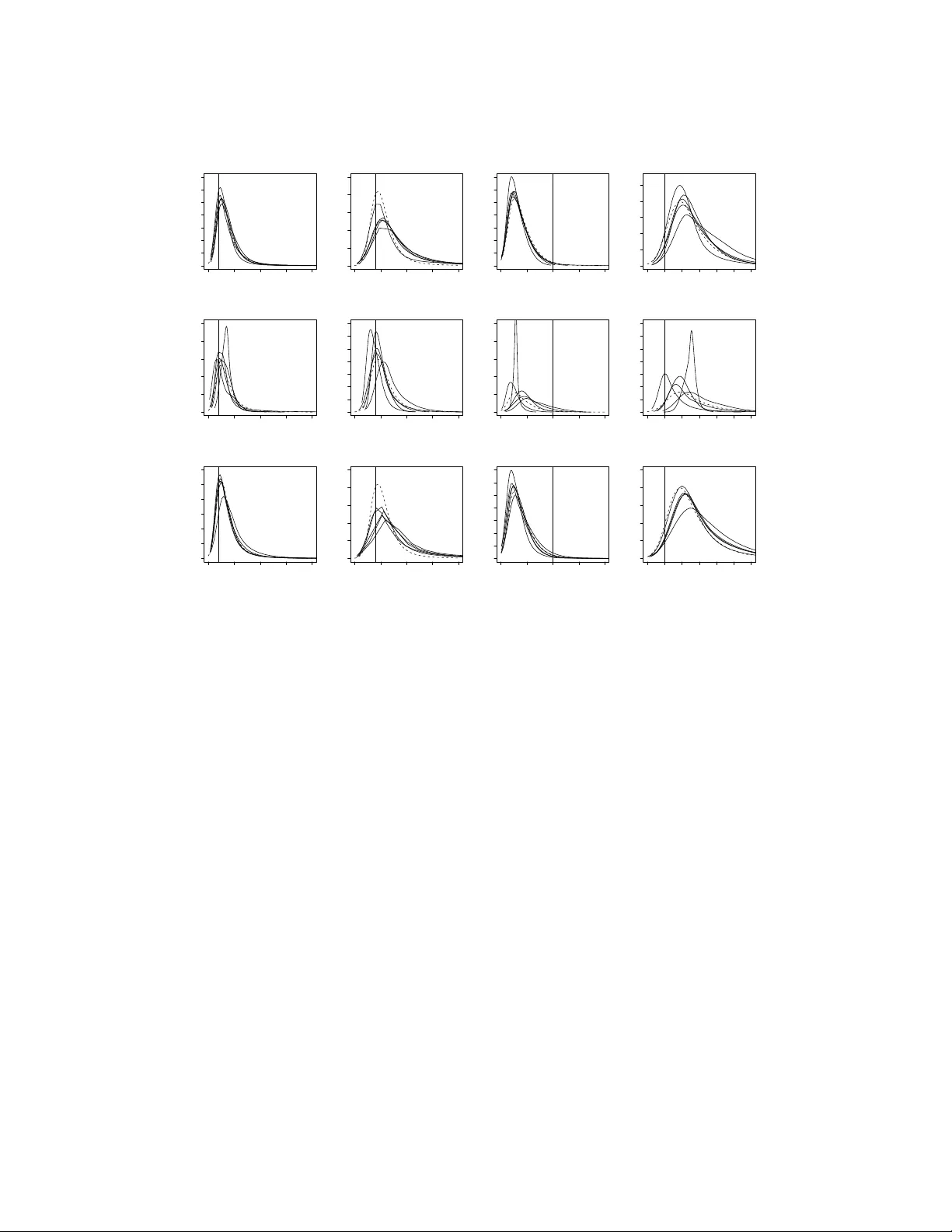
1 2 3 4 5 6 7 8 9 10 11 12 13 14 15 16 17 18 19 20 21 22 23 24 25 26 27 28 29 30 31 32 33 34 35 36 37 38 39 40 41 42 43 44 45 46 47 48 Biometrika (2024), xx , x, pp . 1–9 C  2007 Biometrika T rust Printed in Gr eat Britain Adaptiv e appr oximate Bayesian computation B Y M A R K A . B E AU M O N T School of Biolo gical Sciences, University of Reading, PO Box 68, Whiteknights, Reading RG6 6BX, U .K. m.a.beaumont@reading.ac.uk J E A N - M A R I E C O R N U E T Department of Epidemiology and Public Health, Imperial Colle ge, London SW7 2AZ, U .K. jmcornuet@ensam.inra.fr J E A N - M I C H E L M A R I N Institut de Math ´ ematiques et Mod ´ elisation de Montpellier , Universit ´ e Montpellier 2, Case Courrier 51, 34095 Montpellier cedex 5, F rance Jean-Michel.Marin@uni v-montp2.fr C H R I S T I A N P . R O B E RT Centr e de Recher che en Math ´ ematiques de la D ´ ecision, Universit ´ e P aris Dauphine, 75775 P aris cede x 16, F rance xian@ceremade.dauphine.fr S U M M A RY Sequential techniques can enhance the efficiency of the approximate Bayesian computation algorithm, as in Sisson et al. ’ s (2007) partial rejection control version. While this method is based upon the theoret- ical works of Del Moral et al. (2006), the application to approximate Bayesian computation results in a bias in the approximation to the posterior . An alternativ e version based on genuine importance sampling arguments bypasses this dif ficulty , in connection with the population Monte Carlo method of Capp ´ e et al. (2004), and it includes an automatic scaling of the forw ard kernel. When applied to a population genetics example, it compares fa vourably with two other v ersions of the approximate algorithm. Some ke y wor ds : Markov chain Monte Carlo; partial rejection control; importance sampling; sequential Monte Carlo. 1. I N T R O D U C T I O N When the likelihood function is not a vailable in a closed form, as in population genetics, Pritchard et al. (1999) introduced approximate Bayesian computational methods as a rejection technique bypassing the computation of the lik elihood function via a simulation from the corresponding distribution. Namely , if we observe y ∼ f ( y | θ ) and if π ( θ ) is the prior distrib ution on the parameter θ , then the original approx- imate Bayesi an computation algorithm jointly simulates θ 0 ∼ π ( θ ) and x ∼ f ( x | θ 0 ) , and accepts the simulated θ 0 if, and only if, the auxiliary variable x is equal to the observed value, x = y . This algorithm is exact in that the accepted θ 0 ’ s are distributed from the posterior . In the more standard occurrence when y is a continuous random v ariable, the approximate Bayesian computation algorithm relies on an approx- imation, where the equality x = y is replaced with a tolerance condition, % ( x, y ) ≤  , % being a measure of discrepancy , for instance a distance between summary statistics, and  > 0 being the tolerance bound. 49 50 51 52 53 54 55 56 57 58 59 60 61 62 63 64 65 66 67 68 69 70 71 72 73 74 75 76 77 78 79 80 81 82 83 84 85 86 87 88 89 90 91 92 93 94 95 96 2 B E AU M O N T , C O R N U E T , M A R I N , A N D R O B E RT The output is then distrib uted from the distribution with density proportional to π ( θ ) pr θ { % ( x, y ) <  } , where pr θ represents the probability distribution of x indexed by a value of θ . This density is denoted by π { θ | % ( x, y ) <  } , where the conditioning corresponds to the marginal distribution of % ( x, y ) given y . Improvements to this general scheme have currently been achieved either by modifying the proposal distribution of the parameter θ to increase the density of x ’ s within a neighbourhood of y (Marjoram et al., 2003; Bortot et al., 2007) or by vie wing the problem as a conditional density estimation and developing techniques to allow for lar ger  (Beaumont et al., 2002). Marjoram et al. (2003) defined a Marko v chain Monte Carlo version of the approximate Bayesian computation algorithm that enjoys the same validity as the original algorithm, namely that, if a Markov chain ( θ ( t ) ) is created via the transition that sets θ ( t +1) equal to a new value θ 0 ∼ K ( θ 0 | θ ( t ) ) only if x ∼ f ( x | θ 0 ) is such that x = y and if u ∼ U (0 , 1) ≤ π ( θ 0 ) K ( θ ( t ) | θ 0 )  π ( θ ( t ) ) K ( θ 0 | θ ( t ) ) , then its sta- tionary distribution is the posterior distribution π ( θ | y ) . Since, in most settings, the distribution of y is absolutely continuous, the abov e constraint x = y is replaced with the approximation % ( x, y ) <  . Example 1. For the toy model studied in Sisson et al. (2007), where θ ∼ U ( − 10 , 10) and x | θ ∼ 0 · 5 N ( θ, 1) + 0 · 5 N ( θ, 1 / 100) , the posterior distribution associated with the observation y = 0 is the normal mixture θ | y = 0 ∼ 0 · 5 N (0 , 1) + 0 · 5 N (0 , 1 / 100) restricted to the set [ − 10 , 10] . As in regular Markov chain Monte Carlo settings, the performance of Marjoram et al. ’ s (2003) algorithm depends on the choice of the scale τ in the random walk proposal, K ( θ 0 | θ ) = τ − 1 ϕ { τ − 1 ( θ − θ 0 ) } , where ϕ is most often a standardised normal or a t density . Howe ver , ev en when τ = 0 · 15 as in Sisson et al. (2007), the Markov chain mixes slowly , but still produces an acceptable fit ov er T = 10 6 iterations. Furthermore, the true target is a vailable here as π ( θ | | x | <  ) ∝ Φ(  − θ ) − Φ( −  − θ ) + Φ { 10(  − θ ) } − Φ {− 10(  + θ ) } and, for the value  = 0 · 025 , it is indistinguishable from the exact posterior density π ( θ | y = 0) . W e can thus clearly separate the issue of poor con ver gence of the algorithm, depending on τ , from the issue of approximating the posterior density , depending on  . Sisson et al. (2007) modified the approximate Bayesian computation algorithm using partial rejection control, introduced in Liu (2001). The method is sequential in that simulated populations of N points are generated at each iteration of the algorithm and that those populations are exploited to produce better proposals for a giv en target distribution in later iterations. As demonstrated in Douc et al. (2007), the re- liance on earlier populations to build proposals preserves con vergence properties provided an importance sampling perspective is adopted. W e also recall that a progressiv e improvement in the performance of proposals is the appeal of using a sequence of samples, rather than a single one. The sequential feature of the problem is augmented by the fact that the tolerance  is decreasing with iterations, being chosen either from a deterministic scale or from quantiles of earlier iterations as in Beaumont et al. (2002). Sisson et al. ’ s (2007) algorithm produces samples ( θ ( t ) 1 , · · · , θ ( t ) N ) by using, at iteration t = 1 , a re gular approximate Bayesian computation step and, at each iteration t = 2 , . . . , T , Marko v transition kernels K t for the generation of the θ ( t ) i ’ s, namely θ ( t ) i ∼ K t ( θ | θ ? ) , until x ∼ f ( x | θ ( t ) i ) is such that % ( x, y ) <  , where θ ? is selected at random among the pre vious θ ( t − 1) i ’ s with probabilities ω ( t − 1) i ( i = 1 , . . . , N ) . The probability ω ( t ) i is deriv ed by an importance sampling argument, ω ( t ) i ∝ π ( θ ( t ) i ) L t − 1 ( θ ? | θ ( t ) i ) { π ( θ ? ) K t ( θ ( t ) i | θ ? ) } − 1 , (1) where L t − 1 is an arbitrary transition kernel. In their examples, Sisson et al. (2007) use L t − 1 ( θ 0 | θ ) = K t ( θ | θ 0 ) , which means that the weights are all equal under a uniform prior . The ratio (1) is inspired from Del Moral et al. (2006) who use a sequence of backward kernels L t − 1 in a sequential Monte Carlo algorithm to achie ve unbiasedness, up to the renormalisation effect, in the marginal distribution of the current value without computing this intractable mar ginal. 97 98 99 100 101 102 103 104 105 106 107 108 109 110 111 112 113 114 115 116 117 118 119 120 121 122 123 124 125 126 127 128 129 130 131 132 133 134 135 136 137 138 139 140 141 142 143 144 Adaptive appr oximate Bayesian computation 3 In this paper , we show via both theoretical and experimental arguments that the weight (1) is biased. Moreov er, we introduce a population Monte Carlo correction to the algorithm. It is based on genuine importance sampling arguments and we demonstrate its applicability as well as the improv ement it brings compared with the partial rejection control version. W e also illustrate its efficienc y in a population genetics example, when compared with two standard alternati ves. 2. B I A S O F T H E PA RT I A L R E J E C T I O N C O N T RO L V E R S I O N 2 · 1 . Distribution of the partial r ejection contr ol sample In order to establish the bias in the weight (1) as clearly as possible, we consider the limiting case when  = 0 . In that case, both Pritchard et al. ’ s (1999) and Marjoram et al. ’ s (2003) algorithms are correct sam- plers from π ( θ | y ) . The corresponding partial rejection control version selects a θ ( t − 1) from the pre vious sample and then generates both θ 0 ∼ K t ( θ | θ ? ) and x ∼ f ( x | θ 0 ) until x = y . T o properly ev aluate the bias associated with one step of Sisson et al. ’ s (2007) algorithm, we also assume that the previous sample is correctly generated from the target, i.e. that θ ? ∼ π ( θ | y ) . Then, denoting by θ ( t − 1) the selected θ ? , the joint density of the accepted pair ( θ ( t − 1) , θ ( t ) ) is proportional to π ( θ ( t − 1) | y ) K t ( θ ( t ) | θ ( t − 1) ) f ( y | θ ( t ) ) , where the normalisation constant only depends on y . Using (1), the weighted distribution of θ ( t ) is such that, for an arbitrary integrable function h ( θ ) , E { ω t h ( θ ( t ) ) } is proportional to Z Z h ( θ ( t ) ) π ( θ ( t ) ) L t − 1 ( θ ( t − 1) | θ ( t ) ) π ( θ ( t − 1) ) K t ( θ ( t ) | θ ( t − 1) ) π ( θ ( t − 1) | y ) K t ( θ ( t ) | θ ( t − 1) ) f ( y | θ ( t ) ) d θ ( t − 1) d θ ( t ) ∝ Z Z h ( θ ( t ) ) π ( θ ( t ) ) L t − 1 ( θ ( t − 1) | θ ( t ) ) π ( θ ( t − 1) ) K t ( θ ( t ) | θ ( t − 1) ) π ( θ ( t − 1) ) f ( y | θ ( t − 1) ) × K t ( θ ( t ) | θ ( t − 1) ) f ( y | θ ( t ) ) d θ ( t − 1) d θ ( t ) ∝ Z h ( θ ( t ) ) π ( θ ( t ) | y )  Z L t − 1 ( θ ( t − 1) | θ ( t ) ) f ( y | θ ( t − 1) ) d θ ( t − 1)  d θ ( t ) with all proportionality terms being functions of y only . Therefore we can conclude that there is a bias in the weight (1) unless the inner function integrates in θ ( t − 1) to the same constant for all values of θ ( t ) . Apart from this special case, which is achiev able when L t − 1 ( θ ( t − 1) | θ ( t ) ) = g ( θ ( t − 1) ) but not in the random walk type proposal when L t − 1 ( θ ( t − 1) | θ ( t ) ) = ϕ ( θ ( t − 1) − θ ( t ) ) , (1) is incorrect since the weighted output is not distributed from π ( θ | y ) . Paradoxically , the weight (1) used in this partial rejection control version misses a f ( y | θ ( t − 1) ) term in its denominator , while the method is used when f ( y | θ ) is not av ailable. This is exactly the difference between the weights used in Sisson et al. (2007) and those used in Del Moral et al. (2006), namely that, in the latter paper , the posterior π ( θ ( t − 1) | y ) e xplicitly appears in the denominator instead of the prior . The accept-reject principle at the core of approximate Bayesian computation allo ws for the replacement of the posterior by the prior in the numerator of the ratio (1), but not in the denominator . 2 · 2 . A mixtur e illustration When using the standard version of the algorithm that includes an additional approximation due to the tolerance zone % ( x, y ) <  , there is no reason for the bias to vanish, ev en though experiments show that the bias in the weights (1) for the tolerance target π { θ | % ( x, y ) <  } generally decreases as  increases, which agrees with the fact that the limiting case is the prior . The following example illustrates this point: Example 1. For the mixture target and a normal random walk k ernel K t , the first row of Figure 1 sho ws the output of fi ve consecutiv e iterations of Sisson et al. ’ s (2007) algorithm, using a decreasing sequence of  t ’ s, from  1 = 2 down to  5 = 0 · 01 , and a standard deviation in K t equal to τ = 0 · 15 . Clearly , using this algorithm leads to a bias in terms of the tolerance target for all values of  t , the tails being poorly cov ered. In contrast, using a much larger τ = 1 / 0 · 15 results in a good fit of the tolerance target, as shown by Figure 2 in Sisson et al. (2007). This fit does not contradict the bias exhibited abov e since using 145 146 147 148 149 150 151 152 153 154 155 156 157 158 159 160 161 162 163 164 165 166 167 168 169 170 171 172 173 174 175 176 177 178 179 180 181 182 183 184 185 186 187 188 189 190 191 192 4 B E AU M O N T , C O R N U E T , M A R I N , A N D R O B E RT −3 −1 1 3 0.0 0.2 0.4 0.6 0.8 1.0 −3 −1 1 3 0.0 0.2 0.4 0.6 0.8 1.0 −3 −1 1 3 0.0 0.2 0.4 0.6 0.8 1.0 −3 −1 1 3 0.0 0.2 0.4 0.6 0.8 1.0 −3 −1 1 3 0.0 0.2 0.4 0.6 0.8 1.0 −3 −1 1 3 0.0 0.2 0.4 0.6 0.8 1.0 −3 −1 1 3 0.0 0.2 0.4 0.6 0.8 1.0 −3 −1 1 3 0.0 0.2 0.4 0.6 0.8 1.0 −3 −1 1 3 0.0 0.2 0.4 0.6 0.8 1.0 −3 −1 1 3 0.0 0.2 0.4 0.6 0.8 1.0 Fig. 1. Histograms of the weighted samples of size M = 5 × 10 3 produced by five consecutiv e uses of (1) on the first row and the population Monte Carlo version on the second row , for the mixture target, with  t = 2 , 1 . 5 , 1 , 0 · 5 , 0 · 01 , using for both rows the scale τ = 0 · 15 . The ex- act posterior density is plotted as a dotted curve, while the target of the simulation algorithm, π { θ | % ( x, y ) <  } , is represented by full lines. Both densities are identical in the last column. a large scale in the proposal K t very closely amounts to using a flat prior distribution. The corresponding normal density is then almost constant in the interval [ − 3 , 3] that supports the posterior distribution. For τ = 1 / 0 · 15 , using the weight (1) is thus equiv alent to Pritchard et al. ’ s (1999) original algorithm and therefore as inefficient for this tar get. 3. C O R R E C T I O N V I A I M P O RTA N C E S A M P L I N G A N D P O P U L A T I O N M O N T E C A R L O 3 · 1 . P opulation Monte Carlo Since the missing factor in (1) is the unkno wn likelihood f ( x | θ ( t − 1) ) , a first resolution of the problem is to resort to an estimation of the lik elihood based on earlier samples. But a standard importance sampling perspectiv e allows for a more direct approach, in a spirit similar to the population Monte Carlo algorithm of Capp ´ e et al. (2004). 193 194 195 196 197 198 199 200 201 202 203 204 205 206 207 208 209 210 211 212 213 214 215 216 217 218 219 220 221 222 223 224 225 226 227 228 229 230 231 232 233 234 235 236 237 238 239 240 Adaptive appr oximate Bayesian computation 5 Since the t -th iteration sample is produced from the proposal distribution ˆ π t ( θ ( t ) ) ∝ N X j =1 ω ( t − 1) j K t ( θ ( t ) | θ ( t − 1) j ) , a natural importance weight associated with an accepted simulation θ ( t ) i is ω ( t ) i ∝ π ( θ ( t ) i )  ˆ π t ( θ ( t ) i ) . The unbiasedness of this correction results from the identity E { ω ( t ) h ( θ ( t ) ) } ∝ Z h ( θ ( t ) ) π ( θ ( t ) ) ˆ π ( θ ( t ) ) ˆ π ( θ ( t ) ) f ( θ ( t ) | y ) ˜ π ( θ ( t − 1) ) d θ ( t ) d θ ( t − 1) , which does not depend on the distribution ˜ π of the θ ( t − 1) j ’ s. As in the original population Monte Carlo method, the fact that K t may depend on simulations from earlier iterations does not jeopardise the validity of the method. In addition, Douc et al. (2007) proved that K t must be modified at each iteration for the iterations to bring an asymptotic improvement on the Kullback–Leibler diver gence between the proposal ˆ π t and the target: for instance, if the variance of the random walk does not change from one iteration to the next, the approximation of the tar get by ˆ π t does not change either and it is then more ef ficient to run a single iteration with twice as many points. Since ˆ π t is an approximation to the distribution of the sample simulated at iteration t , when marginalised against all previous samples, this version of the approximate Bayesian computation algorithm can be interpreted as an approximate version of the sequential Monte Carlo algorithm of Del Moral et al. (2006), when using the optimal backward kernel. When considering component-wise independent random walk proposals, K t ( θ ( t ) k | θ ( t − 1) k ) = τ − 1 k ϕ { τ − 1 k ( θ ( t ) k − θ ( t − 1) k ) } for each component θ ( t ) k of the parameter vector θ ( t ) , the asymptotically optimal choice of the scale f actor τ k is av ailable. Indeed, when using a Kullback–Leibler measure of div ergence between the target and the proposal, E log " π ( θ ( t ) | y )  Y k τ − 1 k ϕ { τ − 1 k ( θ ( t ) k − θ ( t − 1) k ) } f ( y | θ ( t ) ) , #! where the expectation E is taken under the product distribution ( θ ( t ) , θ ( t − 1) ) ∼ π ( θ ( t ) | y ) × π ( θ ( t − 1) | y ) , the minimisation of the Kullback diver gence leads to the component-wise maximisation of E [log τ − 1 k ϕ { τ − 1 k ( θ ( t ) k − θ ( t − 1) k ) } ] under the product distribution π ( θ ( t ) | y ) × π ( θ ( t − 1) | y ) . The optimal scale is then equal to E { ( θ ( t ) k − θ ( t − 1) k ) 2 } , that is, τ 2 k = 2 var ( θ k | y ) , under the posterior distrib ution. The implementation of this updating scheme on the scale is straightforward. The algorithmic rendering of the corresponding optimised population Monte Carlo scheme is thus as follows: P opulation Monte Carlo appr oximate Bayesian computation: Giv en a decreasing sequence of tolerance thresholds  1 ≥ · · · ≥  T , 1. At iteration t = 1 , For i = 1 , ..., N Simulate θ (1) i ∼ π ( θ ) and x ∼ f ( x | θ (1) i ) until % ( x, y ) <  1 Set ω (1) i = 1 / N T ake τ 2 1 as twice the empirical variance of the θ (1) i ’ s 2. At iteration 2 ≤ t ≤ T , For i = 1 , ..., N , repeat Pick θ ? i from the θ ( t − 1) j ’ s with probabilities ω ( t − 1) j generate θ ( t ) i | θ ? i ∼ N ( θ ? i , τ 2 t ) and x ∼ f ( x | θ ( t ) i ) 241 242 243 244 245 246 247 248 249 250 251 252 253 254 255 256 257 258 259 260 261 262 263 264 265 266 267 268 269 270 271 272 273 274 275 276 277 278 279 280 281 282 283 284 285 286 287 288 6 B E AU M O N T , C O R N U E T , M A R I N , A N D R O B E RT until % ( x, y ) <  t Set ω ( t ) i ∝ π ( θ ( t ) i ) / P N j =1 ω ( t − 1) j ϕ n τ − 1 t “ θ ( t ) i − θ ( t − 1) j ”o T ake τ 2 t +1 as twice the weighted empirical variance of the θ ( t ) i ’ s The expression of the importance weight ω ( t ) i in volves a sum of N terms and, therefore, the computa- tional cost of this step of the population Monte Carlo approximate Bayesian computation algorithm is in O ( T N 2 ) . Howe ver , in realistic applications of approximate Bayesian computations, the main cost is as- sociated with the pre vious step, namely the repeated simulations from the sampling density . For instance, in the population genetics example, the algorithm spends at least 95% of the computing time in the repeat loop and less than 5% of the time on the remaining computations. 3 · 2 . A mixtur e illustration Example 1. For the mixure target, using the population Monte Carlo version leads to a recovery of the target, whether using a fixed standard deviation τ = 0 · 15 as shown on the second row of Figure 1, or τ = 1 / 0 · 15 , or a sequence of adaptiv e τ t ’ s as in the above algorithm. The graphical difference between these implementations is genuinely difficult to spot; the estimated variance stabilises very quickly in this toy example. 3 · 3 . A population genetics e xample This example considers a simple e volutionary scenario of two populations having di verged from a common ancestral population. Data consists of the genotypes at fiv e microsatellite loci of 50 diploid individuals from each of the populations. Loci are assumed to ev olve according to the strict stepwise mutation model: when a mutation occurs, the number of repeats of the mutated gene increases or decreases by one unit with equal probability . Once di verged, populations do not exchange gene and there is no migration. The natural parameters of this model are the three ef fective population sizes, N 1 , N 2 and N anc , the time of diver gence ( t div ) and the mutation rate ( µ ) assumed here to be common to all loci. While the analyses will be performed with these natural parameters, only identifiable combinations of those, such as the three parameters θ 1 = 4 N 1 µ , θ 2 = 4 N 2 µ and θ a = 4 N anc µ , and the parameter τ div = t div µ , will be considered in the output. In this experiment, se veral simulated datasets hav e been produced using the software dev eloped by Cornuet et al. (2008), with the following parameter values: N 1 = N anc = 10 , 000 , N 2 = 2 , 000 , t div = 1 , 000 and µ = 0 · 0005 , out of which one is presented in this paper , b ut identical conclusions were dra wn from the other datasets. The tolerance region { % ( x, y ) <  } used in the approximate Bayesian computation schemes is based on twelve summary statistics as in Cornuet et al. (2008), namely mean number of alleles, mean genic div ersity , mean size v ariance and mean Garza-W illiamson M index for each population sample, F S T and ( δ µ ) 2 distances between population samples, and mean probability of assignment of each sample to the other population. The distance % ( x, y ) is then chosen as the Euclidean distance between the observed and the simulated summary statistics, normalised by their standard deviation under the predicti ve model. The deri vation of the distance thus requires a preliminary e valuation of those standard de viations for each summary statistic by simulation. Each dataset has been submitted to three parallel analyses: a standard approximate Bayesian computa- tion analysis follo wing Beaumont et al. (2002), performed via Cornuet et al. ’ s (2008) software, a tempered Markov chain Monte Carlo analysis as described in Bortot et al. (2007), and a population Monte Carlo analysis. In each case, the same prior distributions hav e been used, consisting in a U [10 2 , 10 5 ] prior on the three ef fective sizes, a U [10 , 10 4 ] prior on the time of div ergence, and a U [10 − 4 , 10 − 3 ] prior on the muta- tion rate. In addition, since Beaumont et al. ’ s (2002) algorithm includes a final local regression adjustment, this adjustment has been performed on the output of both alternativ e algorithms. In order to operate a fair comparison between the three methods, the computing times are kept identi- cal. Thus, reference posterior distributions have been constructed with Beaumont et al. ’ s (2002) approach, using N = 3 × 10 4 simulated datasets and choosing  as the 0 · 01 quantile of the distances. F or Bortot et 289 290 291 292 293 294 295 296 297 298 299 300 301 302 303 304 305 306 307 308 309 310 311 312 313 314 315 316 317 318 319 320 321 322 323 324 325 326 327 328 329 330 331 332 333 334 335 336 Adaptive appr oximate Bayesian computation 7 0 50 100 150 200 0.000 0.015 0.030 θ θ 1 0 5 10 15 20 0.00 0.10 0.20 θ θ 2 0 10 20 30 40 0.00 0.06 0.12 θ θ a 0.0 1.0 2.0 3.0 0.0 0.4 0.8 τ τ div 0 50 100 150 200 0.00 0.02 0.04 θ θ 1 0 5 10 15 20 0.00 0.15 0.30 θ θ 2 0 10 20 30 40 0.0 0.2 0.4 θ θ a 0.0 1.0 2.0 3.0 0.0 1.0 2.0 3.0 τ τ div 0 50 100 150 200 0.000 0.015 0.030 θ θ 1 0 5 10 15 20 0.00 0.10 0.20 θ θ 2 0 10 20 30 40 0.00 0.06 0.12 θ θ a 0.0 1.0 2.0 3.0 0.0 0.4 0.8 τ τ div Fig. 2. V ariability of the dif ferent alternativ e schemes e val- uated though fiv e replicates of the density estimates of the posterior distributions of four identifiable parameters of the population genetics model. First line: population Monte Carlo version; second line: tempered Marko v chain Monte Carlo version; third line: Beaumont et al. ’ s (2002) ver- sion of the approximate Bayesian computation algorithm, against the reference posterior , obtained by 5 × 10 5 sim- ulations in Beaumont et al. ’ s (2002) version (dotted line). The vertical lines identify the true values of the parameters. al. ’ s (2007) approach, the tuning parameter driving the acceptance threshold  is drawn from an e xponen- tial prior with parameter equal to the mean distance of the ten closest datasets (among 5000 generated in a pilot simulation), followed by 23 , 000 regular iterations with a thinning factor of 23 . Each Markov move combined two simultaneous updates : an independent draw of  from its exponential prior and a random walk based on a log-normal de viate with standard de viation equal to 0 · 3 of one of the other parame- ters chosen uniformly at random, the latter in volving the computation of a Hastings term. Lastly , in the population Monte Carlo version,  1 is based on the preliminary simulation as the 0 · 1 quantile and four iterations are performed with  2 = 0 · 75  1 ,  3 = 0 · 9  2 and  4 = 0 · 9  3 , and with truncated normals in the random walk. Each iteration is based on samples of size 10 3 . All three versions then require an aver - age 4 · 5 minutes. Figure 2 summarises the output of the comparison between the three methods ov er five independent runs for the same simulated dataset and it shows that, at least in this example, the posterior ev aluations based on population Monte Carlo are more stable than Bortot et al. ’ s (2007) algorithm, while comparable with Beaumont et al. ’ s (2002). 337 338 339 340 341 342 343 344 345 346 347 348 349 350 351 352 353 354 355 356 357 358 359 360 361 362 363 364 365 366 367 368 369 370 371 372 373 374 375 376 377 378 379 380 381 382 383 384 8 B E AU M O N T , C O R N U E T , M A R I N , A N D R O B E RT 4. C O N C L U S I O N While Sisson et al. ’ s (2007) algorithm induces biased weights, with a visible impact on the quality of the approximation, we have sho wn that the same Markov transition kernels and thus the same computing power can be used to produce an unbiased scheme. The population Monte Carlo scheme is based on an importance argument that does not require a back- ward kernel as in (1). W e have thus established that the adaptive scheme of Capp ´ e et al. (2008) is also appropriate in this setting, towards a better fit of the proposal kernel K t to the target π { θ | % ( x, y ) <  } . From a practical point of view , the number of iterations T can be controlled via the modifications in the parameters of K t , a stopping rule being that the iterations should stop when those parameters ha ve settled, while the more fundamental issue of selecting a sequence of  t ’ s towards a proper approximation of the true posterior can rely on the stabilisation of the estimators of some quantities of interest associated with this posterior . A C K N O W L E D G E M E N T S This research is partly supported by the Agence Nationale de la Recherche through the Misgepop project. Both last authors are affiliated with CREST , Paris. Parts of this paper were written by the last author in the Isaac Ne wton Institute, Cambridge, whose peaceful and stimulating en vironment was deeply appreciated. Helpful comments from the editorial board of Biometrika and from O. Capp ´ e are gratefully acknowledged. R E F E R E N C E S B E AU M O N T , M . , Z H A N G , W . & B A L D I N G , D . (2002). Approximate Bayesian computation in population genetics. Genetics 162 , 2025–2035. B O RT O T , P ., C O L E S , S . & S I S S O N , S . (2007). Inference for stereological extremes. J. American Statist. Assoc. 102 , 84–92. C A P P ´ E , O . , D O U C , R . , G U I L L I N , A . , M A R I N , J . - M . & R O B E RT , C . (2008). Adaptive importance sampling in general mixture classes. Statist. Comput. 18 , 447–459. C A P P ´ E , O . , G U I L L I N , A . , M A R I N , J . - M . & R O B E RT , C . (2004). Population Monte Carlo. J. Comput. Graph. Statist. 13 , 907–929. C O R N U E T , J . - M . , S A N T O S , F., B E AU M O N T , M . A . , R O B E RT , C . P ., M A R I N , J . - M . , B A L D I N G , D . J . , G U I L L E - M AU D , T. & E S T O U P , A . (2008). Inferring population history with DIY ABC: a user-friendly approach to Approx- imate Bayesian Computation. Bioinformatics 24 , 2713–2719. D E L M O R A L , P . , D O U C E T , A . & J A S R A , A . (2006). Sequential Monte Carlo samplers. J . Royal Statist. Society Series B 68 , 411–436. D O U C , R . , G U I L L I N , A . , M A R I N , J . - M . & R O B E RT , C . (2007). Con ver gence of adaptive mixtures of importance sampling schemes. Ann. Statist. 35(1) , 420–448. L I U , J . (2001). Monte Carlo Strategies in Scientific Computing . Springer-V erlag, Ne w Y ork. M A R J O R A M , P . , M O L I T O R , J . , P L A G N O L , V . & T A V A R ´ E , S . (2003). Markov chain Monte Carlo without likelihoods. Pr oc. Natl. Acad. Sci. USA 100 , 15324–15328. P R I T C H A R D , J . K . , S E I E L S TA D , M . T., P E R E Z - L E Z AU N , A . & F E L D M A N , M . W . (1999). Population growth of human Y chromosomes: a study of Y chromosome microsatellites. Mol. Biol. Evol. 16 , 1791–1798. S I S S O N , S . A ., F A N , Y . & T AN A K A , M . (2007). Sequential Monte Carlo without lik elihoods. Pr oc. Natl. Acad. Sci. USA 104 , 1760–1765.