Network Capacity Region of Multi-Queue Multi-Server Queueing System with Time Varying Connectivities

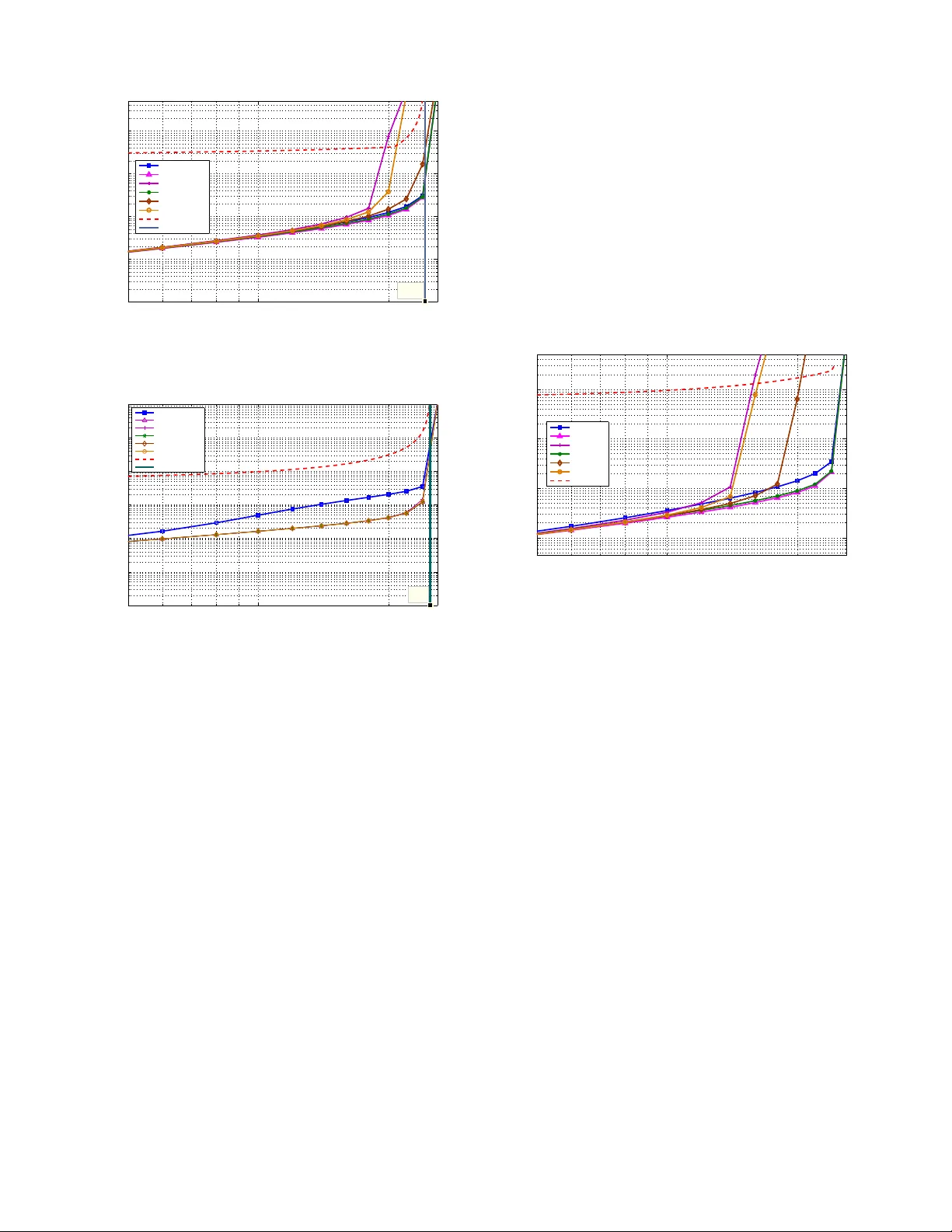
Netw ork Capacity Re gion of Multi-Queue Multi-Serv e r Queueing Sys tem with T ime V arying Connecti vities Hassaa n Halabian, Ioannis Lambadaris, Chung-Horng Lu ng Department of Systems a nd Computer En gineering Carleton Uni versity , 1125 Colonel By Dri ve, Ottawa, ON, K1S 5B6 Ca nada Email: { hassanh, ioannis.lambadaris, ch ung-horng.lung } @sce.carleton.c a Abstract —Network capacity r egion of multi-queue multi-server queueing system with random ON-OFF connectivities and sta- tionary arriv al processes is deriv ed in this paper . S pecifically , th e necessary and sufficient cond itions for the stability of the system are derived u nder general arriv al processes with finite first and second moments. In the ca se of stationary arrival processes, these conditions establish the n etwork capacity region of the system. It is also shown that AS /LCQ (Any Serv er/Longest Connected Queue) policy stabilizes the sy stem when it is stabilizable. Furthermore, an upper bou nd for the av erage qu eue occupancy is deriv ed for this policy . I . I N T R O D U C T I O N Resource allocation is one of th e main concerns in the design pro cess of emerging wireless networks. Ex amples of such network s are OFDMA and CDMA wireless systems in which orth ogonal resou rces (OFDM subcar riers an d CDMA codes) must be allo cated to mu ltiple u sers. Research in th is area foc uses o n findin g optima l policies to allocate o rthogo nal subchann els to th e users. Th ere ar e stochastic arr i vals for each user which may be buf fered to be transmitted in th e fu ture. Therefo re, the resource allocation problem can b e mo deled as a multi-q ueue m ulti-server que ueing system w ith parallel queues competing for av ailab le servers (which ma y mo del orthog onal subch annels [1], [2], [3], [4], [ 11], [ 15]). Howev er , because of users mobility , en v ironmenta l chan ges, fading and etc., connectivity of each queue to each server is changing with time rand omly . Thu s, we are faced to a multi- queue mu lti- server system with time varying chan nel quality for which we have to design an appr opriate server allocation policy . One of the m ain p erform ance attributes which must be considered for each po licy is its capac ity region and how much this r egion coincides with the network capacity re gion [ 8]. Th e capacity region o f a n etwork is defin ed as the clo sure of th e set o f all ar riv al rate ma trices for which there exists an appropr iate policy that stabilizes the system [8]. This region is uniqu e fo r each network and is in depende nt of resour ce alloca tion policy . On the other hand, the capacity region o f a specified p olicy , say π , is the clo sure of the set of all arrival rate matrices for which π re sults into the stability o f the system. Obviou sly , 1 This w ork wa s supported by Mathematics of Information T echnolo gy and Comple x Systems (MIT A CS) and Natura l Sciences and Enginee ring Research Council of Canada (NSERC). the capac ity region of any policy is a subset of the n etwork capacity region. In fact, the network capac ity region of a system is the union of the capacity r egions of all the possible resource allo cation p olicies w e can hav e fo r a network [8]. A po licy that achieves th e network capac ity region is c alled thr ou ghput o ptimal . The stab ility prob lem in wireless que ueing networks was mainly addre ssed in [6], [7], [8], [9]. In [6], author s introduced the capac ity region of a qu eueing network. They consider ed a time slotted system in their work and assumed that arriv al processes are i.i.d. sequen ces and the qu eue length pr ocess is a Mar kov proc ess. They also char acterized the network capacity region o f multi-queue single-server system with time varying ON-OFF con nectivities which is described by some condition s on th e a rriv al traffic [7]. They also proved that for a symmetric system ( with the same ar riv a l and connectivity statistics for all the queues), LCQ ( Longest Con nected Queue) policy maximizes the capacity region and also provid es the optimal p erforman ce in terms of av erage q ueue o ccupancy (o r equiv alently average delay) [7]. In [8], [9] and [ 13], the notion of network capacity region of a wireless network was intro- duced for mo re general arriv al a nd queue length p rocesses. Furthermo re, L yapun ov dr ift techn iques were applied in [8] and [9] to analy se the stability of the prop osed policies for stochastic optimization problems in wireless n etworks. The prob lem of server allocation in mu lti-queue multi- server systems with tim e varying connectivities was main ly addressed in [1], [2 ], [3], [4], [1 1]. In [2], Max imum W eight (MW) policy , a throu ghput optimal server allocation p olicy for stationary connectivity processes was prop osed. Howe ver , [2] does n ot explicitly me ntion the conditions on the arriv al traffic to g uarantee th e stability of MW . References [1], [3], [4], [11] study the optimal server allocation problem in terms of a verage delay . In [1], [3], [4 ], author s argue that in general, achieving instantaneou s th roughp ut and load balancing is impossible in a policy . Howe ver, as they sho w this goal is attainab le in th e special case of ON-OFF connectivity pro cesses. They also in- troduced the MT LB ( Maximum- Throug hput Lo ad-Balancing ) policy a nd showed th at this policy is minimizin g a class of cost function s inclu ding total average de lay for the case o f two symmetric qu eues (with the same arriv al and c onnectivities statistics). [1 1] considers this problem for g eneral num ber of symmetric queues and servers. Authors in [1 1] ch aracterized a class o f Most Bala ncing (MB) policies among all work conservin g po licies which are minimizing a class o f cost function s including total average delay in sto chastic ord ering sense. They used stochastic or dering and dy namic coupling ar- guments to show the op timality o f M B p olicies for sym metric systems. In this pap er , we will cha racterize the capacity region of multi-queu e m ulti-server queu eing system with ran dom ON-OFF con nectivities and stationary arriv al p rocesses ba sed on th e sto chastic p roperties of the system. T ow ard this, the necessary and suf ficient cond itions fo r the stability of the system is der iv ed under a g eneral arr i val process with finite first a nd seco nd moments. For stationary arr i val pr ocesses, these conditions establish the network capacity region of the system. W e also showed th at a simp le server allocation policy called AS/LCQ maximizes th e capacity region i.e. its cap acity region coincide with th e network capacity region and ther efore it is a throughp ut optimal po licy . It is worth mentioning th at AS/LCQ acts exactly the same as MW policy p roposed in [2] when the connectivity pro cess is ON-OFF in MW . The rest of the p aper is organized as follows. Sectio n II describes th e mode l and notation r equired thr ough the p aper . In section I II we d iscuss about the str ong stability definition in que ueing networks and L yapunov drift technique briefly . Then, we will d erive n ecessary and sufficient co nditions for the stability o f ou r m odel a nd also find an upp er bo und fo r th e av erage queu e oc cupancy . In section I V we p resent simulatio n results and compare stability and delay performanc es o f some heuristic work-conser ving po licies with th ose of AS/LCQ and the u pper boun d obtained in sectio n III. Sec tion V summ arizes the conclusion s of the paper . I I . M O D E L D E S C R I P T I O N Our model in this paper is the same as the m odel used in [1], [2], [ 3], [4], [11] with ON- OFF conn ecti vity p rocesses. W e consider a time slotted queu eing system with equal length time slots and eq ual length pac kets. The model co nsists of a set o f par allel queues L an d a set of id entical servers K . Each server can serve at mo st one pac ket at each time slot and we d o n ot allow server sharing by th e queues. In o ther words, each server can serve at most one queu e a t each time slot. Assum e that |L| = L and |K| = K . At each time slot t , th e link between each queue i ∈ { 1 , ..., L } and server j ∈ { 1 , ..., K } is eithe r connected or disconnected . Assume that connectivity process b etween queue i an d server j is mode lled by an i.i.d . binary rando m process which is deno ted by G ij ( t ) , i.e. G ij ( t ) ∈ { 0 , 1 } . Su ppose that p ij represents the expected value of this process, i.e. E [ G ij ( t )] = p ij . There are also exogenou s arrival processes to the q ueues in set L . Assum e that the ar riv a l p rocess to each queue i at tim e slot t (i.e. the number of packet arrivals du ring time slot t ) is r epresented by A i ( t ) . For these p rocesses we assume that E [ A 2 i ( t )] < A 2 max < ∞ fo r all t . Each queu e has an infinite buffer sp ace i.e. we do not have pac ket drop s. W e assume that the new arriv als are added to e ach queue at the end of eac h time slot. Let X ( t ) = ( X 1 ( t ) , ..., X L ( t )) be the queue length p rocess vector at the end of time slot t af ter ad ding new arrivals to the queues. Figure 1 sho ws the model used in th is paper . A server sch eduling policy at ea ch time slot should decide on h ow to allocate servers from set K to the qu eues in set L . This must b e acco mplished ba sed on the av ailable inf ormation about the conn ectivities G ij ( t ) an d also the q ueue length process X ( t ) . ) ( 1 t X ) ( t X L ) ( 2 t X ) ( 11 t G ) ( 1 t G K ) ( 21 t G ) ( 2 t G K ) ( t G LK ) ( 1 t G L ) ( 1 t A ) ( 2 t A ) ( t A L Fig. 1: Mu lti-queue multi-server qu eueing system with time varying conne cti vities I I I . S TA B I L I T Y O F M U LT I - Q U E U E M U LT I - S E RV E R S Y S T E M W I T H T I M E V A RY I N G C O N N E C T I V I T I E S In this section, we will conside r the stability problem of multi-que ue mu lti-server system with ON-OFF connectivities for which we will find th e n ecessary and sufficient co n- ditions for its stability . W e also show that AS/LCQ (Any Server/Longe st Con nected Queu e) policy will stabilize the system as lon g as it is stabilizable. Th e details of th is po licy will be presented in part D o f this section. At first, we will have a revie w on the notio n of strong stability in qu eueing networks. A. S tr ong Stab ility W e begin with in troducin g th e d efinition of strong stability for a queu eing system [8], [9]. Oth er definitions can be foun d in [5], [6], [7], [1 4]. Consider a discrete time single queu e system with an arr i val process A ( t ) and service process µ ( t ) . Assume that the arri vals ar e added to the system at the end of each time slot. W e ca n see that the qu eue leng th proce ss X ( t ) at time t evolves with time accord ing to the following ru le. X ( t ) = ( X ( t − 1) − µ ( t )) + + A ( t ) (1) where ( · ) + outputs the term in side the br ackets if it is nonnegative and is zer o otherwise. Strong stability is given by the following definition [8]. Definition 1: A q ueue satisfying the cond itions ab ove is called str ongly stable if lim sup t →∞ 1 t t − 1 X τ =0 E [ X ( τ )] < ∞ (2) Naturally for a queu eing sy stem we ha ve the fo llowing definition [8]. Definition 2: A que ueing system is called to b e stro ngly stable if all th e queues in the system ar e strongly stable. In o ur work we use th e strong stability definition and fro m now we use “stability” and “strong stability” interchang ably . The following importan t property of stro ngly stable q ueues giv es an inv aluable insight of th e above definition s. Lemma 1 [8]: If a queue is strongly stable a nd either E [ A ( t )] ≤ A for all t or E [ µ ( t ) − A ( t )] ≤ D where A and D a re finite nonnegative constants, then lim t →∞ 1 t E [ X ( t )] = 0 (3) A very imp ortant and u seful mathem atical to ol used in network stability an alysis and sto chastic co ntrol/op timization of wireless networks is Lyapunov Drift technique . W e now present a brief revie w of this techniq ue. B. Lyapunov Drift The b asic idea b ehind the L y apunov stability meth od is to define a no nnegativ e function of q ueue back logs in a queueing system which can be seen as a measure of the total a ggregated backlog in the system at time t . Then we e valuate the “dr ift” of such function in two su ccessi ve time slots by taking the ef fect of our co ntrol decision (schedulin g or resource allocation policy) in to accou nt. I f the expected value of the drift is negativ e as the b acklog g oes b eyond a fixed thresh old, then the system is stable. This is the meth od used in [8], [9], [12], [10], [1 3], [14] to prove the stability of the systems workin g under their proposed policies. For a queu eing system with L queues and qu eue length vector X ( t ) = ( X 1 ( t ) , ..., X L ( t )) , the following quadr atic L yapu nov function has b een used in liter ature ([8], [9], [12], [13], [14]). V ( X ) = L X i =1 X 2 i ( t ) (4) Assume that E [ X i (0)] < ∞ , ∀ i = 1 , 2 , ..., L and X ( t ) e volves with some p robabilistic law (not necessarily Mar kovian). Then, the following impo rtant lem ma holds. Lemma 2 [8]: If there exist con stants B > 0 an d ǫ > 0 such that for all time slots t we have E [ V ( X ( t + 1)) − V ( X ( t )) | X ( t )] ≤ B − ǫ L X i =1 X i ( t ) , (5) then the system is strongly stable and further we have lim sup t →∞ 1 t t − 1 X τ =0 L X i =1 E [ X i ( τ )] ≤ B ǫ (6) The left hand side of expression (5) is u sually called L yapu nov dr ift function wh ich is a measur e of expected v alue of chang es in the b acklog in two successi ve time slots. W e can easily see the id ea behind L yapun ov method in stabilizing queuein g systems fr om Lemma 1. It is no t hard to show that, when the aggregated back log in the system go es beyond th e bound B ǫ , then the L y apunov drift in the left h and sid e of (5) will be negativ e, meanin g that the system r eceiv es a n egati ve drift o n the expected ag gregated b acklog in two successiv e time slots. In other words the system tends toward lower backlog s and this results in its stability . C. Necessary Con dition for th e Stability o f the System Let h ik ( t ) be th e departure process at time slot t from queu e i to server k . Then, we c an have th e following equation for the q ueue leng th process which shows the ev olution of queu e length process with time. X i ( t ) = X i ( t − 1) − K X k =1 h ik ( t ) + A i ( t ) (7) T o find the necessary cond ition for the stability of th e system, we need to use the fo llowing lemma. Lemma 3 : If the system is strong ly stable unde r some server allocation policy π , th en for each queue i lim t →∞ 1 t t X τ =1 E [ A i ( τ )] = lim t →∞ 1 t t X τ =1 K X k =1 E [ h ik ( τ )] , (8) i.e. for a stable system th e average e xpected arr i vals to a queu e is equal to th e average expected dep arture f rom that qu eue. Proof: See appendix A. W e now proc eed to find th e necessary cond ition for the stability of the system. Theor em 1: If there e xists a ser ver allocatio n policy π und er which the system is stab le, then lim t →∞ 1 t t X τ =1 X i ∈ Q E [ A i ( τ )] ≤ K − K X k =1 Y i ∈ Q (1 − p ik ) (9) ∀ Q ⊂ { 1 , ..., L } Proof: See appendix B. Remark: If the ar riv a l proc esses A i ( t ) ’ s are stationary , then E [ A i ( t )] = λ i for all t an d therefore the left han d side of (9) will be equal to P i ∈ Q λ i . Conseq uently , the necessary condition f or th e stability of the sy stem with stationary arriv al processes would be X i ∈ Q λ i ≤ K X k =1 (1 − Y i ∈ Q (1 − p ik )) ∀ Q ⊂ { 1 , ..., L } . (10) D. Su fficient Cond ition fo r the S tability of the S ystem W e can d i vide th e server allo cation po licy in our mod el into two schedu ling problem s. First, we should determ ine the or der under which servers are selected fo r service and second , f or each server decide to allo cate it to a pa rticular queue. Consider the po licy th at cho oses an arb itrary orderin g o f servers and then for each server , allocates it to its long est con nected queue (LCQ). In other words, in this policy we d o not r estrict ourselves with a specific ordering of servers and we accept any permutatio n of the servers accord ing to which servers will be selected for serv ice. Ho wev er , for the ne xt phase of schedu ling, for each selected server we use the LCQ policy . W e call such a po licy as AS/LCQ (Any Server/Lon gest Conn ected Queue). W e will n ow derive the sufficient condition for the stability of o ur model and prove that AS/LCQ stabilizes the system as long as condition (1 1) is satisfied. An up per b ound is also derived for th e time averaged expected numb er of packets in the system. Theor em 2: The multi-q ueue m ulti-server system is stable under AS/LCQ if for all t X i ∈ Q E [ A i ( t )] < K − K X k =1 Y i ∈ Q (1 − p ik ) ∀ Q ⊂ { 1 , ..., L } . (11) Furthermo re, the following bou nd for the average expected “aggregate” o ccupancy ho lds. lim sup t →∞ 1 t t − 1 X τ =0 L X i =1 E [ X i ( τ )] ≤ (12) − L 2  LA 2 max + K (2 K − 1)  max Q ⊂{ 1 , 2 ,...,L } ,t    X i ∈ Q E [ A i ( t )] − K + K X k =1 Y i ∈ Q (1 − p ik )    Proof: See appen dix C. It is worth mentioning that AS/LCQ acts exactly the same as MW policy prop osed in [2] when the connectivity proc ess is ON-OFF in MW . Note that for a ll the servers we only use the backlog informa tion at th e beginnin g of each time slot, i.e. during the implementatio n of AS/LCQ po licy at each time slot we do not update the q ueue lengths u ntil all the servers are allocate d at which point we update th e queue lengths. It is interesting to note tha t this p olicy can be non-work con serving at some time slots. In other words, there may exist some idle servers at a time slot while they could hav e served o ther backlogged queues. W e will discuss about it through an examp le in part E o f this section. Remark: Note that by considerin g stationary assumption on the arriv al pro cesses, th e condition (11) would be X i ∈ Q λ i < K − K X k =1 Y i ∈ Q (1 − p ik ) ∀ Q ⊂ { 1 , ..., L } . (13) According to th e definition o f system capa city region and (10) and (13), equ ation (10) character izes th e n etwork capacity region of mu lti-queue multi-server system with stationa ry ON- OFF connectivities and stationary arriv als. E. Discussion As mentioned e arlier , AS/LCQ may exhibit no n-work con - serving behavior d uring some time slots. This can be clarified by the following example. Consider a system with L = 2 and K = 3 with queue length vector X ( t ) = (2 , 1) at time slot t . For the connectivities at this time we hav e the f ollowing matrix. G ( t ) =  1 1 1 0 0 1  Assume th at the o rdering of server selec tion is server 1 first and then server 2 a nd finally server 3. Servers 1 and 2 both are allocated to queue 1 acco rding to LCQ r ule. Server 3 is c onnected to both of the queues. Sin ce in AS/LCQ a ll the servers ar e allocated first an d then the q ueue lengths are updated afterwards, queu e 1 is the longe st conn ected queue for server 3. Thu s, server 3 is allo cated to q ueue 1 as well. Howe ver, queue 1 h as only two packets waiting for service and theref ore server 3 will be idle at this time slot (although it could hav e b een used to serve queu e 2). Note that since AS/LCQ is a no n-work conserving p olicy it can no t be delay optimal. Howev er, it can achieve the network cap acity region as explaine d previously in part D . In fact, AS/LCQ will exhibit non-work conservin g beh aviour in light arriv al loads and as the load incre ases its b ehaviour will converge to work co nserving. Since the capac ity region of a system is m ainly deter mined by its b ehaviour in heavy arriv al loads, this property of AS/LCQ does not h av e conflict with its thro ughpu t op timality . It is worth mentioning that not all work-conser ving po licies are thro ughpu t optima l. In the following section by simulation s we will observe that so me work-conserv ing po licies cann ot ach iev e the network ca pacity region. In the fo llowing section, we will also o bserve that how the serv ice ord ering of servers af fects the av erage total queue occupan cy . Howe ver , as we showed in th e previous par t an arbitrary o rdering is sufficient to achieve the network capacity region. I V . S I M U L A T I O N R E S U LT S Simulation is used to show the validity o f our ana lysis in the pr evious section an d also to co mpare performan ce of AS/LCQ to some heuristic work con serving policies in- cluding LCSF/LCQ (Least Connected Server First/Longest Connected Queue), MCSF/LCQ (Mo st Connected Server First/Longest Con nected Qu eue), LCSF/SCQ (Least Con- nected Server First/Shortest Connected Queu e), MCSF/SCQ (Most Connected Server First/Shortest Connected Queue) and a Randomized policy [1 1]. The LCSF (MCSF) policy at the first phase of scheduling (i.e. dete rmination of servers or der) will sort the ser vers for service accord ing to their number of connectivities in an ascending (descendin g) or der . Th e LCQ (SCQ) p olicy will assign the selected server it to its lo ngest con nected queu e (shortest connected queue). Note that in order to make SCQ policies work conservin g, we only serve the shortest non- empty queues. The Randomized policy at each time slot makes random server selectio ns and fo r each server rand om non - empty queue selection. W e have simu lated a system consisting of 16 queues ( L = 16 ) an d 4 servers ( K = 4 ). First, we considered a symmetric system in which all the arrivals to all th e queu es are the same in d istribution. W e also assumed that con nectivity variables have the sam e distribution (the same co nnectivity probab ilities). In th is system, arriv a ls are assumed to ha ve i.i.d. Bernoulli distributions. Th e capacity region f or these special cases would b e an n dime nsional cube whose side size is equal to K − K (1 − p ) L L which is 0.243 f or p = 0 . 2 and is almost 0.25 for p = 0 . 9 . Figures (2) and (3) show the average total occupan cy of different policies for connectivity probabilities 0.2, and 0 .9 versus arrival rate per q ueue. In th ese figures, it is o bserved that in all th e c ases if the arr i vals are inside the capacity region, AS/LCQ can stabilize th e system and h as av erage to tal occupan cy below the bound we derived in th e previous section. 10 −1 10 −1 10 0 10 1 10 2 10 3 X: 0.243 Y: 0.1014 Arrival Rate Per Queue (Packets/Time Slot) Average Total Occupancy (Packets) AS/LCQ LCSF/LCQ MCSF/SCQ MCSF/LCQ Randomized LCSF/SCQ Bound Capacity Region Fig. 2: A verage T otal Occupan cy for p = 0 . 2 10 −1 10 −2 10 −1 10 0 10 1 10 2 10 3 10 4 X: 0.25 Y: 0.01 Arrival Rate Per Queue (Packets/ Time Slot) Average Total Occupancy (Packets) AS/LCQ LCSF/LCQ MCSF/SCQ MCSF/LCQ Randomized LCSF/SCQ Bound Capacity Region Fig. 3: A verage T otal Occupan cy for p = 0 . 9 W e can fu rther conclud e tha t as the conn ecti vity variable increases th e perf ormance of the work conser ving policies become the same. This agree s with intuition since wh en the system is close to full co nnectivity , any work con serving algorithm will be optim al in terms of average occup ancy and of c ourse better than a ny n on-work c onserving policy like AS/LCQ. Althou gh AS/LCQ ha s larger a verage total occupan cy compa red to other policies, it still stabilizes the system as long as ar riv als are inside the capacity region and has bounded average total occupan cy . Howe ver , this is not th e case for L CSF/SCQ and MCSF/SC Q policies and they cann ot stabilize the system fo r certain arriv als inside th e capacity region. Fro m these figures we a lso see that random ized p olicy perfor ms very close to the oth er policies in these special cases and this is du e to existence o f sy mmetry (in arrivals and connectivities) in these cases. W e have also simulated an asymmetric system in which connectivity variables comes from the following matrix in which p ij = E [ G ij ( t )] . This matrix was ch osen randomly . p =     0 . 9 0 . 2 0 . 2 0 . 8 0 . 2 0 . 1 0 . 5 0 . 6 0 . 8 0 . 1 0 . 1 0 . 9 0 . 02 0 . 5 0 . 8 0 . 8 0 . 9 0 . 02 0 . 5 0 . 99 0 . 3 0 . 8 0 . 78 0 . 99 0 . 8 0 . 03 0 . 9 0 . 87 0 . 5 0 . 98 0 . 62 0 . 4 0 . 2 0 . 72 0 . 86 0 . 3 0 . 66 0 . 21 0 . 84 0 . 03 0 . 1 0 . 65 0 . 65 0 . 1 5 0 . 5 8 0 . 3 2 0 . 69 0 . 12 0 . 02 0 . 4 2 0 . 94 0 . 35 0 . 9 0 . 1 6 0 . 96 0 . 21 0 . 8 1 0 . 7 0 . 09 0 . 1 0 . 45 0 . 1 3 0 . 07     T In this experimen t, arriv als ar e following the Po isson distri- bution with the same rates fo r each slot an d eac h queue. T he capacity region in this case is n ot easy to characterize and describe in a concise manner . Figure (4) sho ws the results for this case. In this figure, we observe that Rando mized policy could not captur e the capacity region wholly . However , LCQ policies (AS/LCQ, LCSF/LCQ and MCSF/LCQ) perfo rms similarly to each other from stab ility point of vie w . 10 −1 10 0 10 1 10 2 10 3 Arrival Rate Per Queue (Packets/Time Slot) Average Total Occupancy (Packets) AS/LCQ LCSF/LCQ MCSF/SCQ MCSF/LCQ Randomized LCSF/SCQ Bound Fig. 4: A verag e total occup ancy for an asymmetric scenario From the above simulations, we can also o bserve that AS/LCQ perfo rms slightly worse as compar ed with other policies in ligh t arr i val loads. This behaviour is because th e fact that AS/LCQ m ay exhibit non -work conserving b ehaviour more frequen tly for light arrival loads. Howe ver, as the load increases AS/LCQ will be work con serving with high prob- ability . W e can also ob serve that the obtaine d boun d is n ot tight. V . C O N C L U S I O N S In this paper we der i ved th e necessary a nd suf ficient condi- tions for the stability o f multi-q ueue mu lti-server system w ith random connectivities an d cha racterized the capacity region of this system for stationar y arri vals. W e also introduced AS/LCQ policy an d argued that alth ough this policy is a non- work co nserving policy , it can stabilize the system for all the arriv als inside th e cap acity region an d th erefore it is a throug hput optimal policy . Then, we d eriv ed an upp er bound of the av erage qu eue occup ancy for th is po licy . Finally , we used simulation s to validate our an alysis and com pare this policy to some work co nserving p olicies in terms of av erage queue occupancy . If we mod ify the policy such that the que ue length s are updated after e ach server is allocated, w e can establish a work conservin g policy . Ho wever , this d oes not increase the capacity region for a system with station ary arrivals. Howe ver , we may help u s to obtain a tighter b ound than we obtained in this work. A P P E N D I X A P R O O F O F L E M M A 3 Proof: I f we write equation (7) for τ = 1 , 2 , ..., t and then adding them up, we will ha ve X i ( t ) = X i (0) − t X τ =1 K X k =1 h ik ( t ) + t X τ =1 A i ( t ) (14) T aking th e expectation f rom both sides, d ividing by t an d th en taking the lim it as t g oes to infinity , we will have the following. lim t →∞ E [ X i ( t )] t = lim t →∞ E [ X i (0)] t − lim t →∞ 1 t t X τ =1 K X k =1 E [ h ik ( t )] + lim t →∞ 1 t t X τ =1 E [ A i ( t )] (15) According t o Lemma 1 and the assumption that E [ X i (0)] < ∞ , the left hand side term and the first term in the right h and side term are eq ual to zero and therefor e the result is proven.  A P P E N D I X B P R O O F O F T H E O R E M 1 Since th e system is strongly stable, (8) mu st be satisfied for any subset of q ueues Q ⊂ { 1 , ..., L } , i.e. lim t →∞ 1 t t X τ =1 X i ∈ Q E [ A i ( τ )] = lim t →∞ 1 t t X τ =1 X i ∈ Q K X k =1 E [ h ik ( τ )] (16) W e now d efine the sets B k ( τ ) as B k ( τ ) = { G ℓk ( τ ) , X ℓ ( τ − 1) , ℓ ∈ Q } (17) For B k ( τ ) , three disjoint cases are imaginable. B 1 k ( τ ) = { G ik ( τ ) = 0 , i ∈ Q } B 2 k ( τ ) = { G ik ( τ ) = 0 , i ∈ Q } c ∩ { X i ( τ − 1) = 0 , i ∈ Q } B 3 k ( τ ) = { G ik ( τ ) = 0 , i ∈ Q } c ∩ { X i ( τ − 1) = 0 , i ∈ Q } c By co nditionin g each term in the r ight hand side summation in (16) to the e vent B k ( τ ) we have K X k =1 X i ∈ Q E [ h ik ( τ )] = K X k =1 E B k ( τ )   E   X i ∈ Q h ik ( τ ) | B k ( τ )     (18) W e can easily see that E   X i ∈ Q h ik ( τ ) | B j k ( τ )   = 0 j = 1 , 2 (19) and E   X i ∈ Q h ik ( τ ) | B 3 k ( τ )   ≤ 1 (20) Using (19) and (20), eq uation (18) can b e simplified to the following. K X k =1 X i ∈ Q E [ h ik ( τ )] ≤ K X k =1 (1 − P [ B 1 k ( τ )] − P [ B 2 k ( τ )]) (21) Note that P [ B 2 k ( τ )] ≥ 0 and for P [ B 1 k ( τ )] , we have P [ B 1 k ( τ )] = Y i ∈ Q (1 − p ik ) (22) Finally , from (16), (21) an d (22) we conclude th at lim t →∞ 1 t t X τ =1 X i ∈ Q E [ A i ( τ )] ≤ K X k =1 (1 − Y i ∈ Q (1 − p ik )) (23) and the theorem follo ws.  A P P E N D I X C P R O O F O F T H E O R E M 2 Proof: W e will start with the L yapunov f unction e valuation. we will use the quadra tic fu nction (4) a s our L yapunov function . The L ya punov d rift for two successive time slots has the following form . E [ V ( X ( t + 1)) − V ( X ( t )) | X ( t ))] = E " L X i =1 X 2 i ( t + 1) − X 2 i ( t ) | X ( t ) # = E " L X i =1 ( X i ( t + 1) − X i ( t )) 2 | X ( t ) # + 2 E " L X i =1 X i ( t )( X i ( t + 1) − X i ( t )) | X ( t ) # (24) For th e th e first term we ha ve: E " L X i =1 ( X i ( t + 1) − X i ( t )) 2 | X ( t ) # = E " L X i =1 ( A i ( t + 1) − K X k =1 h ik ( t )) 2 | X ( t ) # = E " L X i =1 A 2 i ( t + 1) | X ( t ) # − 2 E " L X i =1 K X k =1 A i ( t + 1) h ik ( t ) | X ( t ) # + E   L X i =1 K X k =1 h ik ( t ) ! 2 | X ( t )   (25) Using the the fact that K X k =1 h ik ( t ) ≥ 0 we get the following inequality L X i =1 K X k =1 h ik ( t ) ! 2 ≤ L X i =1 K X k =1 h ik ( t ) ! 2 ≤ K 2 (26) Since L X i =1 K X k =1 A i ( t + 1) h ik ( t ) ≥ 0 , the first term in (24) can be bounded by E " L X i =1 ( X i ( t + 1) − X i ( t )) 2 | X ( t ) # ≤ L X i =1 E [ A 2 i ( t + 1)] + K 2 (27) Now assume that we select the ser vers for service acco rding to an arbitrar y or der s 1 , s 2 , ..., s K . Thus, for the second term in (24) we hav e E " L X i =1 X i ( t )( X i ( t + 1) − X i ( t )) | X ( t ) # = E " L X i =1 X i ( t )( A i ( t + 1) − K X k =1 h ik ( t + 1)) | X ( t ) # = E " L X i =1 X i ( t ) A i ( t + 1) | X ( t ) # − E " L X i =1 K X k =1 X i ( t ) h is k ( t + 1) | X ( t ) # (28) The first term in (28) can b e written as follows. E " L X i =1 X i ( t ) A i ( t + 1) | X ( t ) # = L X i =1 E [ A i ( t + 1)] X i ( t ) (29) For th e second term in ( 28) we h av e E " L X i =1 K X k =1 X i ( t ) h is k ( t + 1) | X ( t ) # = K X k =1 E " L X i =1 X i ( t ) h is k ( t + 1) | X ( t ) # (30) Now , we introduce the f ollowing n otation. W e sort the queue length process at time slot t in a n ascending or der X q 1 , X q 2 , ...., X q L , i.e. X q i ( t ) ≥ X q i − 1 ( t ) for all i = 2 , ..., L and if X q i ( t ) = X q i − 1 ( t ) , then q i ≥ q i − 1 . Furtherm ore, consider the following d ecompo sition of the connec ti vity pro- cesses for each server k . D k 0 = { G ik ( t + 1) = 0 , f or a l l i ∈ { 1 , ..., L }} D k i = { G q i k ( t + 1) = 1 , G q ℓ k ( t + 1) = 0 , f or i < ℓ ≤ L an d al l i ∈ { 1 , ..., L }} The probability of e vents D k i is gi ven by P ( D k 0 ) = L Y i =1 (1 − p ik ) , P ( D k i ) = p q i k L Y u = i +1 (1 − p q u k ) In the second term of equation (30), each term in the summation can be rewritten as E " L X i =1 X i ( t ) h is k ( t + 1) | X ( t ) # = E " L X i =1 X q i ( t ) h q i s k ( t + 1) | X ( t ) # = L X l =0 E " L X i =1 X q i ( t ) h q i s k ( t + 1) | X ( t ) , D s k l # P ( D s k l ) (31) Note that E " L X i =1 X q i ( t ) h q i s k ( t + 1) | X ( t ) , D s k l # ≥ ( X q l ( t ) − ( k − 1)) + . Therefo re, equatio n (3 1) can be b ounded by E " L X i =1 X i ( t ) h is k ( t + 1) | X ( t ) # ≥ L X l =1 ( X q l ( t ) − ( k − 1)) p q l s k L Y u = l +1 (1 − p q j s k ) = L X l =1 X q l ( t ) p q l s k L Y j = l +1 (1 − p q j s k ) − ( k − 1) L X l =1 p q l s k L Y j = l +1 (1 − p q j s k ) (32) For th e seco nd term in (32) we h av e ( k − 1) L X l =1 p q l s k L Y j = l +1 (1 − p q j s k ) = ( k − 1)   1 − L Y j =1 (1 − p q j s k )   (33) and for the first ter m L X l =1 X q l ( t ) p q l s k L Y j = l +1 (1 − p q j s k ) = L X j =2 ( X q j ( t ) − X q j − 1 ( t ))   1 − L Y l = j (1 − p q l s k )   + X q 1 ( t )   1 − L Y j =1 (1 − p q j s k )   (34) Equation (29) also can be written a s follows. L X i =1 E [ A i ( t + 1)] X i ( t ) = L X l =1 E [ A q l ( t + 1)] X q l ( t ) = L X j =2 ( X q j ( t ) − X q j − 1 ( t )) L X l = j E [ A q l ( t + 1)] + X q 1 ( t ) L X l =1 E [ A q l ( t + 1)] (35) Using eq uations (28)-(30) an d (32)-(3 5) we have the fo l- lowing bo und fo r the second ter m in (24). E " L X i =1 X i ( t )( X i ( t + 1) − X i ( t )) | X ( t ) # ≤ L X j =2 ( X q j ( t ) − X q j − 1 ( t )) L X l = j E [ A q l ( t + 1)] + X q 1 ( t ) L X l =1 E [ A q l ( t + 1)] − L X j =2 ( X q j ( t ) − X q j − 1 ( t )) K X k =1   1 − L Y l = j (1 − p q l s k )   − X q 1 ( t ) K X k =1   1 − L Y j =1 (1 − p q j s k )   + K X k =1 ( k − 1)   1 − L Y j =1 (1 − p q j s k )   ≤ L X j =2 ( X q j ( t ) − X q j − 1 ( t )) ·   L X l = j E [ A q l ( t + 1)] − K X k =1   1 − L Y l = j (1 − p q l s k )     + X q 1 ( t ) L X l =1 E [ A q l ( t + 1)] − K X k =1   1 − L Y j =1 (1 − p q j s k )     + K X k =1 ( k − 1) (36 ) Now , define m as m = max Q ⊂{ 1 , 2 ,...,L } ,t    X i ∈ Q E [ A i ( t )] − K + K X k =1 Y i ∈ Q (1 − p ik )    Therefo re equation (36) can be bounded by the following. E " L X i =1 X i ( t )( X i ( t + 1) − X i ( t )) | X ( t ) # ≤ L X j =2 ( X q j ( t ) − X q j − 1 ( t )) m + X q 1 ( t ) m + K 2 ( K − 1) = X q L ( t ) m + K 2 ( K − 1) (37) Putting all toge ther and ac cording to (24), (27) and ( 37) the L yapu nov dr ift in equation ( 24) is upper bounded by the following. E [ V ( X ( t + 1)) − V ( X ( t )) | X ( t ))] ≤ L X i =1 E [ A 2 i ( t + 1)] + K 2 + 2 X s L ( t ) m (38) + K ( K − 1) = L X i =1 E [ A 2 i ( t + 1)] + 2 K 2 − K − ǫ ( LX s L ( t )) (39 ) where ǫ = − 2 m L . According to conditio n (1 1), m is negati ve, therefor e ǫ > 0 . Since P L i =1 X i ( t ) ≤ L X s L ( t ) , th erfore − ǫ ( LX s L ( t )) ≤ − ǫ P L i =1 X i ( t ) . Conseque ntly the L yapun ov drift (38) is bounded by E [ V ( X ( t + 1)) − V ( X ( t )) | X ( t ))] ≤ LA 2 max + 2 K 2 − K − ǫ L X i =1 X i ( t ) = B − ǫ L X i =1 X i ( t ) (40) in which B that has positiv e v alue is defined as B = LA 2 max + 2 K 2 − K (41) Therefo re, accord ing to Lemm a 2 , the multi-queue multi- server system is stab le und er AS/LCQ as long as conditio n (11) is satisfied a nd also the time average expected co ngestion in the system is bounded b y lim sup t →∞ 1 t t − 1 X τ =0 L X i =1 E [ X i ( τ )] ≤ B ǫ (42) which is equal to (12).  R E F E R E N C E S [1] S. Kitti piyakul and T . Javidi, “Delay-opt imal server allocat ion in multi- queue multi-serv er systems with time-va rying connecti vities, ” IEE E T ransactions on Information Theory , , vol. 55, no. 5, pp. 2319-2333, May 2009. [2] T . Javidi, “Rate stable resourc e alloca tion in OFDM systems: from wate rfilling to queue-balanc ing, ” in Pr oc. Allerton Confer ence on Communicat ion, Contr ol, and Computing 2004. [3] S. Kitti piyakul and T . Javi di, “ A Fresh Look at Optimal Subcarr ier Al- locat ion in OFDMA Systems, ” in Proc . IEE E Confere nce on Decisio n and Contr ol, Dec. 2004. [4] S. Kittipiyakul and T . Javidi, “Resource alloca tion in OFDMA with time-v arying channe l and bu rsty arri vals, ” IEEE Commun. Lett. , v ol. 11, no. 9, pp. 708710, Sep. 2007. [5] S. Asmussen, “ Applie d Pr obabili ty and Queues. ” Ne w Y ork: Spring- V erlag, Second ed., 2003. [6] L . T assiulas and A. Ephremides, “Stabi lity prope rties of constrained queuein g systems and scheduli ng policies for maximum throughput in multihop radio net works, ” IEEE T ransactions on Auto matic Contr ol , vol. 37, No. 12, pp. 19361949, December 1992. [7] L . T assiula s and A. Ephremides, “Dynamic server allocation to parall el queues with randomly v arying connecti vity , ” IEEE T ransactions on Informatio n Theory , vol. 39, No. 2, pp. 466478, 1993. [8] L . Geor giadis, M. J . Neely and L. T assiula s, “Resou rce Allocation and Cross Layer Control in W irele ss Netw orks, ” No w Publisher , 2006. [9] M. J. Neely , “Dyna mic powe r allocati on and rout ing for satel lite and wireless netw orks with time varying channels, ” Ph.D. dissertat ion, Massachuset ts Institut e of T echnology , LIDS, 2003. [10] P .R. Kumar and S.P . Meyn, “Stabili ty of queueing network s and scheduli ng policies, ” IEEE Tr ansactio ns on Automati c Contr ol. , Feb . 1995. [11] H. Al-Zubaidy and I. Lambadaris and I. V inioti s, “Optimal Resource Scheduli ng in W ireless Multi-servic e S ystems With Random Chann el Connect i vity , ” (to appear in) Proc eeding of IEEE Global Communica- tions Confer ence (GLOBECOM 2009) , No v . 2009. [12] N. McKeo wn, A. Mekkittik ul, V . Anant haram, and J. W alran d, “On Achie ving 100% thro ughput in an input-queued switch , ” IEEE T rans- actions on Communications, v ol. 47, pp. 126012 72, August 1999. [13] M. J. Neely , E. Modiano , and C. E. Rohrs, “Dynamic power alloca tion and routing for time va rying wireless networks, ” IEEE J ournal on Selec ted Ar eas in Communicati ons, Spec ial Issue on W ire less Ad-hoc Network s , vol. 23, No. 1, pp. 89103, Januar y 2005. [14] E. Leonardi , M. Melia, F . Neri, and M. Ajmone Marson, “Bounds on av erage delays and queue size ave rages and v ariance s in input-queued cell-b ased switches, ” Pr oceedin gs of IEEE INFOCOM, , 2001. [15] A. Ganti, E. Modiano and J. N. Tsitsiklis, “Optimal transmission scheduli ng in symmetric communication models with intermitt ent connec ti vity , ” IEEE T ransactions on Information Theory , , vol. 53, Issue 3, March 2007.