On the number of $k$-cycles in the assignment problem for random matrices

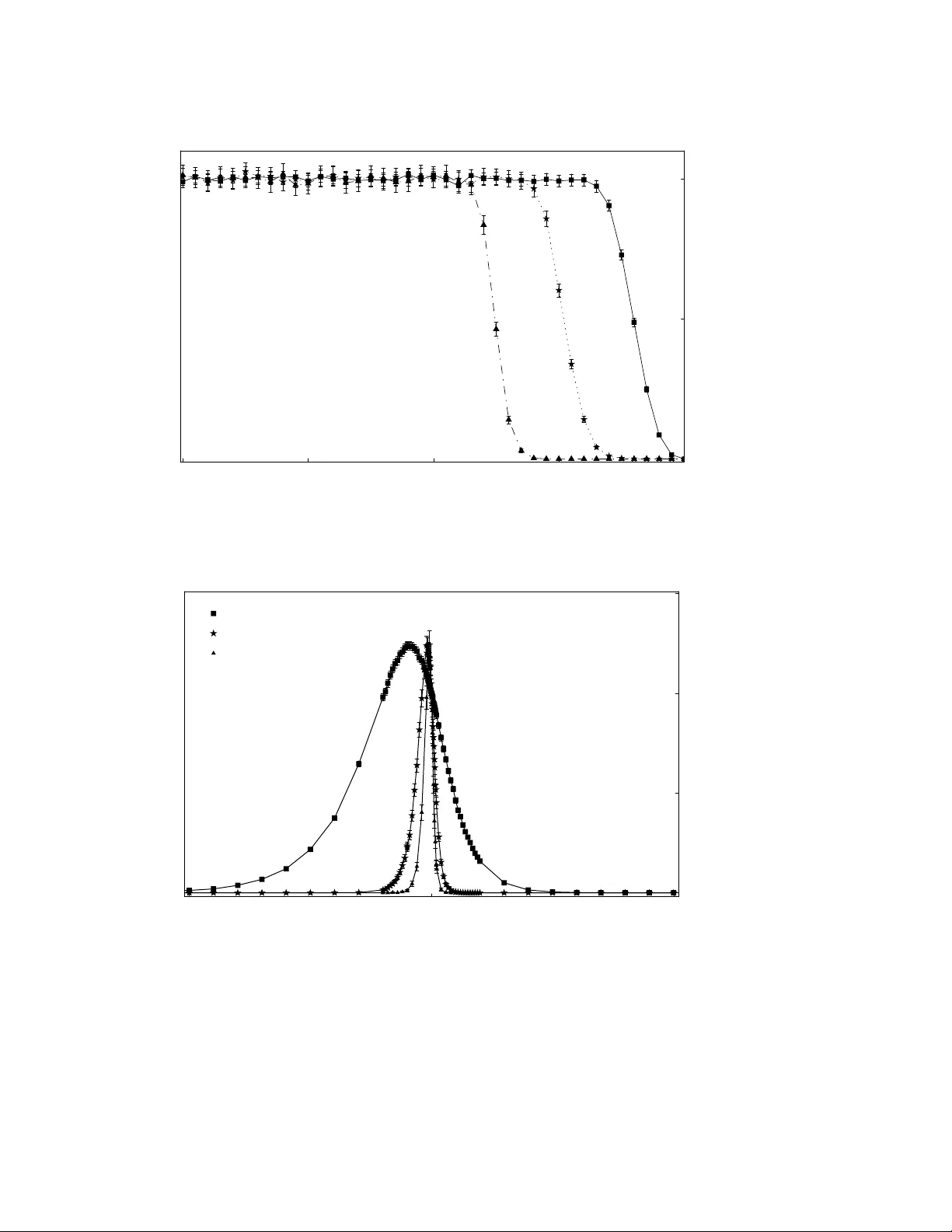
On the number of k -cy cles in the assignment pr oblem f or random matrices Jos ´ e G. Estev e and Fer nando F alceto Departa mento de F ´ ısica T e ´ orica, Faculta d de Ciencias and Institut o de Bioco mputaci ´ on y F´ ı sica de sistemas complejos. Uni ver sidad de Zaragoza , E-50009 Zaragoza (Spain ) E-mail: esteve@unizar.e s and falceto@ unizar.es Abstract. W e continue the stud y of the assignment problem for a random cost matrix. W e analyse the number of k -cycles for the s olution and their dependenc e on the s ymmetry of the random matrix. W e observe that for a symmetric matrix o ne and two-cy cles a re dominant in the o ptimal solution. In the antisymmetric case the situation is the opposite and the one and tw o-cy cles are suppressed. W e solv e the model for a pure random matrix (without corre latio ns between its entries) and giv e analyti c ar guments to explai n the numerical results in the symmetric and antisymmetr ic ca se. W e sho w that the results can be expla ined to great accurac y by a simple ansatz that connect s the expe cted number of k -cycles to that of one and two cycle s. P A CS numbers: 02.60.Pn, 02.70.Rr , 64.60.Cn 1. Introduction The assignment pr ob lem (AP) f or a given cost or d istance ‡ matrix ( d i j ) , ( i , j = 1 , . . . , N ) consists in finding the perm utation σ ∈ S N that minimises the total distance ∑ N i = 1 d i σ ( i ) . There are o ther prob lems related to th is with ad ditional c onstraints on the p ermutation s allowed. Pro bably , th e mo st renowned one is the traveling salesman pr o blem ( TSP) th at can be formulated like th e pre vious AP b ut ad mitting on ly cyclic permutations (we insist that unlike in the standard TSP ou r matrix do es not need to be a true distance matrix) . The list includes also the min imum weight simple matching pr o blem (SMP) w here on ly perm utations composed of tw o -cycles are allowed (o bviously in this case N has to be ev en) an d the, somehow opposite case of the minimu m weight dir ected 2-restricted 1-factor pr o blem (1FP), for which one-cycles and two-cycles ar e forb idden. If the matrix is symm etric the latter problem can be also seen as a minimum weight non dir ec ted 2-factor pr oblem (2FP). From the po int of v iew of complexity theory , it is well known (see [ 1]-[4]) that th e TSP is NP-hard while the 2FP the AP and the SMP can be solved in a time the scales poly nomially with N . In this pap er we are inter ested in the study of th e AP fo r rando m cost o r distance matrices. This problem has been studied for many years, fo cusing mainly o n the minimal distance D ( AP ) . For example, for rando m matrices whose entries have pro bability de nsity ‡ W e use the term distance matrix although d i j are not necessa rily t rue distances in a mathemati cal sense , i n partic ular the y do not need to be positi ve or symm etric. On the number of k -cy cles in the assignment problem for random matrices 2 ρ ( d i j ) = exp ( − d i j ) θ ( d i j ) ( θ is th e Hea viside step function ), it was first con jectured by G. Parisi [5] and then proved rigor ously ([6 ]-[9]) that the expected length is h D ( AP ) i = N ∑ m = 1 1 m 2 , (1) with N the number of points to be matched. Furtherm ore, for general random distances whose densities behave like ρ ( r ) = 1 − ar + O ( r 2 ) n ear r = 0, it is known ([10]-[14]) that h D ( AP ) i = ζ ( 2 ) − 2 ( 1 − a ) ζ ( 3 ) + 1 N + O ( N − 2 ) , (2) where ζ ( x ) is the Riemann’ s zeta function. It is also kn own that for the TSP on symmetric random matr ices with ρ ( 0 ) = 1, the mean length of the minimal tour is ([15 ],[16]) D 0 = lim N → ∞ h D ( T S P ) i = 2 . 041 ..., and the next 1 / N correction s are ([17 ],[18]) h D ( T S P ) i = D 0  1 − 0 . 1437 N − 10 . 377 N 2 + · · ·  . (3) Different probab ilistic relations amon g the problem s considered in the previous paragra phs are also well known in the literature. Name ly , since the seminal work of Karp [19] we know that for pu rely asymmetric ran dom matrices with un iformly distributed entries we have lim N → ∞ ( h D ( T S P ) i − h D ( AP ) i ) = 0 . See also [20] and referen ces therein for more precise est imates of this conv ergence. The case of symmetric r andom matrices is howe ver different, and in this situation th e expected length of the solu tion in the TSP and in the A P do no t coincide in the large N lim it. A different problem that h as been sh own to be closer to the TSP in pr obabilistic terms is th e, above mentio ned, 2FP where one-cycles and two-cycles are excluded . In ref. [21] it is shown that the expected v alue of the minimal distance for TSP and 2FP with s ymmetric r andom matrix coincid es in the large N limit. These results m ake clear that the structur e of cycles in the o ptimal permu tation for the AP d epends strong ly on the sym metry of th e distan ce matrix and gives the clue to compa re, at a probabilistic le vel, the different related problems. Actually , in a recen t paper [22], we foun d that de pending on th e char acteristics of the d istance matrix the AP can interp olate between tho se situation s which ar e ne ar the SM problem (in the sense that the op timal perm utation is com posed appro ximately of N / 2 c ycles) and those whose optimal perm utation is composed of a few cycles (just one in some cases) and one and two cycles are absent. These can be con sidered n ear the TSP or 2FP solution. The transition between bo th limits is governed by the cor relation of th e distances d i j and d ji : for positive corr elations the A P problem is in the “SM regime”, wh ereas for anti corr elated distances it is “n ear” the TSP r egime. The tr ansition point is located where there is no correlation betwe en the entr ies d i j (that is all the distan ces are i ndepen dent random variables), a situation that can be solved analytically as we shall see. In this paper we shall study the expected num ber of k -cycles in the o ptimal permu tation and its dependence o n the symmetry of the distance matrix. W e shall show analy tic and numerical results with special emphasis in t he large N limit. In particular we put into relation the probability of a permutation to b e the solution of the AP with the n umber of one-cycles an d two-cycles it co ntains. This ansatz can account for the numerical results with high accuracy . The p aper is organised as follo ws. I n th e next section we describe the problem with full precision . The numerical results for the expected value o f the numb er o f k -cycles are presented in section 3 . I n the next three sections we give an alytic arguments to explain the On the number of k -cy cles in the assignment problem for random matrices 3 numeric results in the thre e regimes: the pu re rando m case, the antisym metric region and the symmetric one. W e finally end th e paper with some comments and conclusions. 2. Description of the problem Giv en an N × N matrix M = ( d i j ) we are interested in the permutation σ ∈ S N that minimises the total distance D σ = N ∑ i = 1 d i σ ( i ) This prob lem is usually named as the assignment problem or bipartite matching problem . The novelty of o ur appro ach is th at rather than lookin g at the minimum distance itself we focus on the permutation σ that gives this minimum. Mor e co ncretely we are i nterested in the number o f k -cycles, p k , k = 1 , . . . , N in the per mutation σ (note tha t this numb ers, determine the conjugacy class of σ inside S N ). From this poin t of view we shall con sider equiv alent those matrices M whose m inimum total distance correspond s to permutation s in the same conjugacy class. This implies the following equi valence relation: i ) ( d i j ) ∼ ( α d i j + c ) , α , c ∈ R , α > 0 ii ) ( d i j ) ∼ ( d π ( i ) π ( j ) ) π ∈ S N iii ) M = ( d i j ) ∼ M t = ( d ji ) . (4) In this p aper M is a ra ndom matrix that d epends o n a constant λ , we sometim es den ote it by M λ , and it is con structed in the fo llowing way: take a r andom N × N m atrix R = ( R i j ) whose entries ar e equally distributed, independ ent, real r andom v ariab les with probab ility density ρ , then the entries of M λ = ( d i j ) ar e given by d i j = R i j + λ R ji . Note that, unlike the others, th e diagon al elem ents depend on a sing le random variable and read d ii = ( 1 + λ ) R ii . Observe that M λ is sym metric for λ = 1, antisym metric fo r λ = − 1 an d purely rando m (without any corre lation among its entries) for λ = 0. From the definition of M λ we have M 1 / λ = 1 λ M t λ , and, therefo re M λ ∼ M 1 / λ for λ > 0 and M λ ∼ − M 1 / λ for λ < 0. As it was mentioned before we are interested in the number of k -cycles p k or r ather in its expected value in th e distribution generated by R , we c all it P k ( λ ) = h p k i λ . W e sha ll consider λ ∈ [ − 1 , 1 ] that ranges from th e antisymmetr ic matrix for λ = − 1 to the symmetric one for λ = 1. On th e other han d, given th e previous equiv alen ce ( M λ ∼ M 1 / λ for λ > 0), the results with λ ∈ ( 0 , 1 ] r epeat themselves fo r 1 / λ . Then in an effectiv e way we cover the whole positi ve real line. For the negati ve part thin gs are dif ferent as we hav e M λ ∼ − M 1 / λ for λ < 0; but, if the probability den sity for the entries of R is such that ρ ( x ) = ρ ( c − x ) f or s ome constant c , then the distrib ution of the optimal permutation wit h λ ∈ [ − 1 , 0 ) is again identical to the one for 1 / λ . In the n ext section s we shall presen t the results for P k ( λ ) and h n c i λ , where n c = ∑ k p k is the tota l nu mber of cycles in the o ptimal permu tation. It is interestin g to observe how they change with λ from the an tisymmetric point, λ = − 1, to the symm etric one, λ = 1. Dif ferent values for the dimension N ar e considered to study the large N limit. On the number of k -cy cles in the assignment problem for random matrices 4 W e als o vary the d istribution ρ used to define the model. W e mainly focus on the unifor m distribution between [ 0 , 1 ] , with density ρ u , and on the exponential one, ρ e ( x ) = exp ( − x ) θ ( x ) . Note that ρ u ( x ) = ρ u ( 1 − x ) and then, in this p articular case, the in terval [ − 1 , 1 ] for λ is enough to cover the whole r eal line. On the other han d, as mentioned in th e previous section, ρ e has be en exten si vely used in stud ies of th e assignm ent pro blem for r andom matr ices [5],[1 6] which motiv ates our choice. The two d istributions considered in the previous paragrap h h av e the same lim it for the density in th e min imum o f its suppor t ρ u ( 0 ) = ρ e ( 0 ) = 1. Many of the r esults ob tained in the next sections hold indepe ndently of the distrib ution used to gener ate the ran dom matrix provided its d ensity functio n have a n on zero limit in the minimum of its sup port. The same proper ty is inv oked in [5],[16] to h ave a minimal distance with finite limit when N goes to infinity . 3. Numerical results. W e carried ou t a numerical sim ulation o f the statistical en semble descr ibed in the p revious section. F o r th at we gen erated b etween 10 5 and 10 6 random instances f or M λ , using the correspo nding probability d istributions for t he elemen ts R i j . Th e number of instances depends on the dimension of the matrix, which ranges from N = 40 to N = 1200 . Once we genera te the ma trix M λ we solve the assignment problem for it u sing the algorithm of R. Jon ker and A. V olgenan t [3] and compute the number of k -cycles p k obtained in this way . In Fig. 1 we plot the value of h n c i = ∑ k P k ; there one can see the phase transition between the two regimes of h n c i for λ < 0 and λ > 0. In the first case ( λ < 0) the expected value of n c behaves like log ( N ) an d is (almo st) constant with λ . For λ > 0 the values of h n c i grow linearly with N an d λ [22]. T o und erstand the behaviour o f h n c i in both regimes we analyse sep arately the average number of k -cycles, P k , as a fu nction of λ and k . In the rest of the section we present the values obtained in the numerical simulation. In the following sections we shall give a theoretical explanation of these results. i) On e cycles: In the second plot ( Fig. 2) we show P 1 as a fu nction of λ for different values of the dimension N . The dots correspo nd to ρ = ρ u for dimensio ns 40, 2 00, 400 , 800 and 12 00. The joined p lots represen t the results fo r ρ = ρ e with N = 40 , 200 an d 1 200. W e show no error bars because these are ne gligible. W e observe that P 1 vanishes in all cases in the left part of the diagram, it attains a common value P 1 = 1 fo r λ = 0 and finally it takes a value that grows like √ N for λ = 1. W e finally note that the join ed plo ts, correspondin g to a dif ferent prob ability density ρ = ρ e , lay very close to their respective dots (for ρ = ρ u ) and the fit gets better as N grows. The scaling of P 1 with √ N is shown in th e inset o f Fig. 2 wh ere we p lot P 1 / √ N as a function of λ for different values of N . ii) T wo cycles: In the n ext plo t (Fig. 3) we represent 2 P 2 versus λ . As in the previous case we show it for dif f erent values of the dimension and d ifferent distrib utions: the do ts correspo nd to ρ = ρ u and the joined plots to ρ = ρ e . W e again see that 2 P 2 vanishes near λ = − 1, takes the v alu e 2 P 2 = 1 fo r λ = 0 and grows, in an app roximate ly linear way , in the sym metric region, λ > 0, to a value close to N for λ = 1. W e also observe that the points correspondin g to ρ = ρ u fit very well with those of the jo ined plo t cor respond ing to ρ = ρ e . The inset shows the linear scaling of P 2 with N , fo r N ≥ 200. iii) Thr ee cycles: T he situa tion chan ges drastically when we plot 3 P 3 as a fu nction of λ in Fig. 4. The dots correspond to N = 40, 200 and 1200 for ρ = ρ u . Th e joined plot represents On the number of k -cy cles in the assignment problem for random matrices 5 -0.5 0 0.5 1 λ < > n c 0 20 40 60 80 100 120 N = 40 N = 200 N = 400 N = 800 N = 1200 Figure 1. Mean v alue of the number of cycles of the optimal solution for the assignment problem at different values of λ and N . The dots and the joined plots are obtained with the distributions ρ = ρ u , and ρ = ρ e respecti vely . the case of dimension 1200 with ρ = ρ e . W e see that 3 P 3 gets a constan t v alue equal to 1 for almo st all values of λ and all values of N and ρ . Only n ear λ = 1 th ings depend on N and as N grows the value of 3 P 3 ( λ = 1 ) tends to 1. This limiting behaviour is common for all probability densities ρ . Similar r esults are obtained fo r o ther od d cycles o f small length comp ared to N i.e. 5 P 5 or 7 P 7 are equal to 1 fo r all values of λ except near λ = 1, but it tends to 1 everywhere when N tends to infinity . iv) F o ur cycles. In the next plot ( Fig. 5) we represent the behaviour of four c ycles plotting 4 P 4 versus λ for different v alues of N and ρ . Dots represent the values obtaine d for different dimensions N = 40, 200 and 1 200, all with the unifor m distribution, with d ensity ρ u . The joined plot correspon ds to N = 120 0 with ρ = ρ e . Comparing with t he previous plot of P 3 , we see n o change in the left part, λ < 1. Howe ver the right half is qu ite different. W e o bserve th at P 4 always vanishes at the symmetric point, and it follows a smooth curve (even in the large N limit) f rom 4 P 4 = 1 at λ = 0 to P 4 = 0 for λ = 1. A similar result is obtained f or other sho rt cycles o f even length like P 6 , P 8 , ...: all o f them v anish at λ = 1, only the shape of the curve change s, it is more horizontal near λ = 0 and steeper as we approa ch th e symmetric point. v) Intermediate cycles: I n the Fig. 6 we sho w th e cycles of intermediate length for dimension 200 and the density ρ u . As an example we draw k P k for k = 50 , 10 0 and 150. W e see that, as in previous cases, the b ehaviour for λ < 0 is always constant an d eq ual to 1. For positive λ we see a fast transition from 1 to 0 at a value for λ that d iminishes as k increases. Other interm ediate v alues of k and different values of N or ρ = ρ e giv e similar results (see also Fig. 13 for odd values of k ). vi) N − 1 cycles: In the Fig. 7 we draw ( N − 1 ) P N − 1 for N = 40 , 200 , 400 and ρ = ρ u . W e On the number of k -cy cles in the assignment problem for random matrices 6 N = 40 N = 200 N = 400 N = 800 N = 1200 o o o o o o o o o o o o o o o o o o o o o o o o o o o o o o o o o o o o o o o o o o o o o o o o o o o o o o o o o o o o o o o o o o o o o o o o o o o o o o o o o o o o o o o o o o o o o o o o o o o o o o o o o o o o o o o o o o o o o o o o o o o o o o o o o o o + + + + + + + + + + + + + + + + + + + + + + + + + + + + + + + + + + + + + + + + + + + + + + + + + + + + + + + + + + + + + + + + + + + + + + + + + + + + + + + + + + + + + + + + + + + + + + + * * * * * * * * * * * * * * * * * * * * * * * * * * * * * * * * * * * * * * * * * * * * * * * * * * * * * * * * * * * * * * * * * * * * * * * * * * * * * * * * * * * * * * * * * * * * * * * * * * * + + * * o o N = 200 N = 400 N = 1200 - 0.5 0 0.5 1 0 0.2 0.4 0.6 λ P 1 N -    1 2 - 1 - 0.5 0 0.5 1 0 5 10 15 20 λ P 1 Figure 2. A verage num ber of one-c ycles in the optimal solution for the assignment problem at dif ferent value s of λ and N . The dots are obtained with t he uniform distribution with density ρ = ρ u , and the joined plots with ρ = ρ e . St atistical errors correspondin g to three standard de viation are not visible. The inset sho ws the behav iour of P 1 / √ N as a function of λ for differen t valu es of N . see a peak, sharper as N increases while its max imum moves tow ard λ = 0. I t always takes the unit value at λ = 0. As befo re, different d istributions give similar r esults. Th is plot, as well as those of ( N − 2 ) P N − 2 and ( N − 3 ) P N − 3 which are plotted in the F ig. 9 are qualitativ ely very different from the previous on es and also different fr om each othe r . I n section 5 we shall introdu ce a s imple ansatz that accoun ts for this, with great accuracy . vii) N cycles: Finally in the Fig. 8 we present the results for N P N for different dimensions. Note that it is again constant near λ = − 1 but, contrary to the p revious cases, the constant is no t 1 but rather e 3 / 2 = 4 . 4 816 ... . It takes th e value 1 for λ = 0 and vanishes f or λ > 0. The width of the transition is inverse prop ortional to N . Different distributions give similar results. T o summa rise the results of this section we have that for small cycles, with odd k > 2, kP k ≃ 1 for all λ in the large N limit. Small cycles with ev en k > 2 have a smooth decay to 0 at λ = 1. For cycles of intermediate length kP k ≃ 1 from λ = − 1 until it has an abrup t decay at a positiv e value o f λ that depe nds on k . Cycles of length close to N hav e a very d ifferent behaviour one from each othe r . An d finally , one and t wo c y cles are absent for λ < 0 and gro w like √ N and N respectively for λ > 1. On the number of k -cy cles in the assignment problem for random matrices 7 N = 40 N = 200 N = 400 N = 800 N = 1200 + + + + + + + + + + + + + + + + + + + + + + + + + + + + + + + + + + + + + + + + + + + + + + + + + + + + + + + + + + + + + + + + + + + + + + + + + + + + + + + + + + + + + + + + + + + + + + o o o o o o o o o o o o o o o o o o o o o o o o o o o o o o o o o o o o o o o o o o o o o o o o o o o o o o o o o o o o o o o o o o o o o o o o o o o o o o o o o o o o o o o o o o o o o o o o o o o o o o o o o o o o o o o o o o o o o o o o o o o o o o o o o * * * * * * * * * * * * * * * * * * * * * * * * * * * * * * * * * * * * * * * * * * * * * * * * * * * * * * * * * * * * * * * * * * * * * * * * * * * * * * * * * * * * * * * * * * * * * * * * * * + + * * o o N = 200 N = 400 N = 1200 - 0.5 0 0.5 1 0 0.2 0.4 0.5 λ P 2 N - 1 - 1 - 0.5 0 0.5 1 0 40 200 400 800 1200 λ 2 P 2 Figure 3. A verage n umber of tw o-cyc les (multiplied by 2) in the optimal solution for the assignm ent p roblem at dif ferent v alues of λ and N . The resu lts obtained with the densities ρ u ( ρ e ) are displayed as points ( joined plot) respectiv ely . Statistical errors are negligible. The inset correspon ds to P 2 N versus λ for differen t valu es of N . 4. Solution of the model for λ = 0 . W e start with th e theoretica l study of the model by analysing the p oint λ = 0. In this case M 0 = R and the entries of our matrix are id entical, independent rand om v ariables. Due to this fact we can show th at all p ermutatio ns σ have the same probability o f giving rise to the minimal distance. The proof is very simple. Gi ven M 0 = ( d i j ) call ˆ ρ ( M 0 ) = N ∏ i , j = 1 ρ ( d i j ) , the probab ility distrib ution in the space of matrices for λ = 0. It is th en clear that ˆ ρ (( d i j )) = ˆ ρ (( d π ( i ) j )) , for any p ermutation π ∈ S N . But if σ is th e p ermutation th at min imises the distance D σ for (( d i j )) then σ ◦ π giv es the m inimum distance for ( d π ( i ) j ) . It implies then that σ and σ ◦ π have the same probability of being the optimal permutation , which leads to th e unifor m distrib ution in S N Once we h av e established that at λ = 0 all permutation s h ave the same p robab ility o ur problem is a p urely c ombinato rial one, and r educes to compute how many k -cycles th ere are On the number of k -cy cles in the assignment problem for random matrices 8 -1 -0.5 0 0.5 1 λ 3 P 3 0 0.5 1 N = 40 N = 200 N = 1200 Figure 4. A verage number of 3-c ycles (multiplied by 3) i n the optimal solution for the assignment problem. Symbols correspond t o ρ u and different v alues of N and the joint plot is for ρ e and N = 1200. The error bars correspond to three standard de viations from the mean. -1 -0.5 0 0.5 1 λ 4 P 4 0 0.5 1 N = 40 N = 200 N = 1200 Figure 5. Mean v alue of 4-cycles (multiplied by 4) in the optimal solution for the assignment problem. Symbols correspond to ρ u and different v alues of N and the joint plot is for ρ e and N = 1200. Error bars represent three standard de viations. On the number of k -cy cles in the assignment problem for random matrices 9 -1 -0.5 0 0.5 1 λ k P k 0 0.5 1 k = 50 k = 100 k = 150 Figure 6. A verage number o f k -c ycles (multiplied by k ) in the optimal solution for the assignment problem at dif ferent valu es of k and λ for N = 200. Error bars represent three standard de viations. -0.5 0 0.5 λ H N - 1 L P N - 1 0.5 1 1.5 N = 40 N = 200 N = 400 Figure 7. A verage n umber of ( N − 1)-cycles (times N − 1) in the op timal solution fo r the assignment problem at dif ferent values of λ and N . Error bars represent three standard de viations. Note the c ommon v alue ( N − 1 ) P N − 1 = 1 at λ = 0 for a ll v alues of N . On the number of k -cy cles in the assignment problem for random matrices 10 -1 -0.5 0 0.5 1 λ N P N 0 1 2 3 4 5 N = 40 N = 200 N = 400 Figure 8. A verage numbe r of N -cycles (times N ) in the optimal solution for the assignment prob lem at d ifferent values of λ and N . Er ror bars represent three standard de viations. in S N . This numbe r , that we call ν N ( k ) , is well kn own to be ν N ( k ) = N ! k as one can deriv e from simple countin g arguments, i. e. ν N ( k ) =  N k  ( k − 1 ) ! ( N − k ) ! where the d ifferent factors count repectively th e po ssible choices of k in dexes to form the c y cle, their orderin gs and the permutations of the rest of indexes. Note that in this way e very permutation is counted as many times as the number of k -cycles it contains, hence the result follows. § . For latter purposes we shall p resent here a different, more cum bersome, way to derive ν N ( k ) that makes use of the generating function [23],[25]. L et G ( x ) ≡ ∞ ∑ m = 1 1 m x m = log  1 1 − x  , be the gener ating function fo r the number of k -cycles in S k in the sense that d k d x k     x = 0 G ( x ) = ( k − 1 ) ! . § W e can also use the followi ng iteration ν N ( k ) = ( N − k + δ k 1 ) ν N − 1 ( k ) + ( k − 1 ) ν N − 1 ( k − 1 ) . The first term in the iterati on count s the number of k -c ycles that persist when one add a new index while the seco nd term stands for the number of ways one can add a ne w index to a k − 1-cycl e to make it one unit larger . The δ k 1 is there beca use for one- cycl es, when adding a ne w index linked to itse lf rather than to any of the preexisti ng ones, the number of one-c ycles is increased by one On the number of k -cy cles in the assignment problem for random matrices 11 But we rather want to compute th e nu mber o f k -cycles in S N . T o do th is we observe that the generato r fo r the permutation s in S N are obtained by simply taking the exponential e G = 1 1 − x . The proced ure to obtain the numb er of k -cycles in S N is then simple. W e intro duce G α ( x ) ≡ x + 1 2 x 2 + · · · + 1 k − 1 x k − 1 + α k x k + 1 k + 1 x k + 1 + · · · so that when we take the exponential of G α the p ower of α in every term indicates the number of k -cycles that the corr espondin g permutation contains. Therefeor e, ν N ( k ) is giv en by ν N ( k ) = d d α     α = 1 d N d x N     x = 0 e G α = = d N d x N     x = 0  1 k x k 1 − x  = N ! k . (5) The expected number of k -cycles for λ = 0 is then P k ( λ = 0 ) = ν N ( k ) N ! = 1 k . Note that this result is ind epend ent of N and of the p robab ility density ρ we used to generate the ensemb le. Th is explains why in all the r esults showed in the previous section kP k = 1 for λ = 0. Finally , the expected v alue of n c is: h n c i λ = 0 = N ∑ k = 1 P k ( λ = 0 ) = H N , (6) where H N is the Harmo nic series 5. The antisymmetric region, λ < 0 . In this section we study the behaviour of P k ( λ ) for λ < 0. W e start by the observation that one- cycles and two-cycles are strongly suppressed for λ = − 1. T he absence of on e and two-cycles in the solution of the AP makes it equiv alent to the correspo nding 1FP as it was mentioned in the introductio n. This fact can be heuristically understood if one co nsiders that the optimal permutation for M com es from the cho ice of N eleme ntary distances d i j out of N 2 and, apa rt from the diagonal elements which are 0, the rest of elements are half of them negati ve and half of them positive. Then, for large N , the shortest total d istance will be typic ally obtain ed when we chose only negativ e elements and this excludes the possibility of having one-cycles ( d ii = 0) a nd two- cycles ( d i j = − d ji ) that always include non negati ve en tries. The rest of cycles ha ve no correlation am ong their elements an d there fore it is reasona ble to assume the equipr obability of all permutations that do not con tain o ne-cycles or two-cycles. W ith this assump tion we reduce the problem to a combin atorial one an d we can proceed like in section 3. Our go al, howev er , is to un derstand the expe cted numb er of k -cycles in the whole negativ e region λ ∈ [ − 1 , 0 ] that interpo lates between the ab sence o f on e and two cycles for λ = − 1 to the expected values P 1 ( 0 ) = 1 and P 2 ( 0 ) = 1 / 2 at λ = 0. This goal can be achie ved with the f ollowing ansatz. W e assume that, at least in the large N lim it, the On the number of k -cy cles in the assignment problem for random matrices 12 probab ility for a p ermutation to be the shortest distance depen ds only on the numb er of one- cycles an d two-cycles it contains. This is consistent with the fact that only one and two cycles are sen sible to the symmetry of the matrix, b onds of lo nger cycles are un correlated . Namely for a per mutation with p 1 one-cycles a nd p 2 two-cycles the probab ility is proportio nal to q p 1 1 q p 2 2 , wh ere q 1 and q 2 vanish for λ = − 1 and q 1 = q 2 = 1 fo r λ = 0. The new generating function is then: G q 1 , q 2 ( x ) = q 1 x + q 2 2 x 2 + ∞ ∑ k = 3 1 k x k = log  1 1 − x  + ( q 1 − 1 ) x + ( q 2 − 1 ) x 2 / 2 . That implem ents the id ea o utlined ab ove, as in the expo nential of G q 1 , q 2 ( x ) every term h as a weight q p 1 1 q p 2 2 . Fro m this we derive the normalising factor (the total weigh t of the space of permutatio ns) Ω q 1 , q 2 ( N ) = d N d x N     x = 0 e G q 1 , q 2 = d N d x N     x = 0 e ( q 1 − 1 ) x +( q 2 − 1 ) x 2 / 2 1 − x , (7) while the e xpected v alue for the number of k -cycles can be obtained as in previous section b y introdu cing the factor α multiplying x k and taking the d eriv a tiv e of the exponential at α = 1. The result for k > 2 is P k = Ω q 1 , q 2 ( N ) − 1 1 k d N d x N     x = 0 x k e ( q 1 − 1 ) x +( q 2 − 1 ) x 2 / 2 1 − x for k > 2 . (8) T o comp ute these quantities we use the singularity analysis appro ximation [24]. In the case at hand the N th coefficient in the power series is approxim ated b y the residue at the pole in z = 1. It then gi ves Ω q 1 , q 2 ( N ) = N !  e q 1 + q 2 / 2 − 3 / 2 + O ( | q 1 − 1 | N / N ! + | q 2 / 2 − 1 / 2 | N / 2 / ( N / 2 ) ! )  , and Ω q 1 , q 2 ( N ) P k = N ! k  e q 1 + q 2 / 2 − 3 / 2 + O ( | q 1 − 1 | N − k / ( N − k ) ! + + | q 2 / 2 − 1 / 2 | N / 2 − k / 2 / ( N / 2 − k / 2 ) ! )  . (9) For sm all values of q 1 , q 2 and k ( compare d with N ) this appr oximation can be used and we obtain P k ≈ 1 k for k > 2, which is compatible with th e numerical results of section 3, (see figures 4, 5 and 6). P 1 and P 2 do not follow the ge neral formula but P 1 = Ω q 1 , q 2 ( N ) − 1 d N d x N     x = 0 q 1 x e G q 1 , q 2 ( x ) (10) which, in the singularity analysis approx imation, gi ves P 1 = q 1 + O ( | q 1 − 1 | N − 1 / ( N − 1 ) ! + | q 2 / 2 − 1 / 2 | N / 2 − 1 / 2 / ( N / 2 − 1 / 2 ) ! ) . ( 11) And P 2 = Ω q 1 , q 2 ( N ) − 1 d N d x N     x = 0 q 2 2 x 2 e G q 1 , q 2 ( x ) (12) so that P 2 = q 2 2 + O ( | q 1 − 1 | ( N − 2 ) / ( N − 2 ) ! + | q 2 / 2 − 1 / 2 | N / 2 − 1 / ( N / 2 − 1 ) ! ) . (1 3) On the number of k -cy cles in the assignment problem for random matrices 13 Then for small values of q 1 and q 2 and the values of N we are co nsidering in the paper (f rom 40 to 120 0) we can take P 1 = q 1 and P 2 = q 2 / 2 with a very good accu racy (th at covers the λ < 0 region since there q 1 and q 2 are less than 1). For long cycles k ∼ N the singularity an alysis ap proxim ation is no t valid any more. In this case, ho wev er , it is very easy to com pute (8) explicitly . Th erefore with the pr ecision given by that of Ω q 1 , q 2 ( N ) we get: N P N ≃ e 3 / 2 − q 1 − q 2 / 2 ( N − 1 ) P N − 1 ≃ q 1 e 3 / 2 − q 1 − q 2 / 2 ( N − 2 ) P N − 2 ≃ ( q 2 / 2 + q 2 1 / 2 ) e 3 / 2 − q 1 − q 2 / 2 ( N − 3 ) P N − 3 ≃ ( 1 / 3 + q 1 q 2 / 2 + q 3 1 / 6 ) e 3 / 2 − q 1 − q 2 / 2 (14) - 0.1 0 0.1 0 1. 2. 3. 4. 4.5 Λ N P N - 0.1 0 0.1 0 0.4 0.8 1.2 Λ H N - 1 L P N - 1 - 0.1 0 0.1 0 0.4 0.8 1.2 Λ H N - 2 L P N - 2 - 0.1 0 0.1 0 0.4 0.8 1.2 1.6 Λ H N - 3 L P N - 3 Figure 9. A ve rage number of k P k (for the largest v alues of k ) in the optimal solution for the ass ignment problem at d ifferent v alues of λ and for N = 200. The points are the result of our si mulation and the err or bars represent three standard deviations from the mean. The joined plot is the theoretical prediction using (14). In Fig. 9 we plot kP k for k = N , · · · , N − 3 and N = 2 00. The con tinuous line is th e theoretical value obtained from (14) wh ere we take q 1 = P 1 and q 2 = 2 P 2 . On e ca n see that the agreemen t is e x cellent. A similar match holds for the other cases. Thus, fr om the previous expressions we see th at the beh aviour of P k for for k = 1 , . . . , N for λ ≤ 0 is completely determin ed by q 1 and q 2 . In the rest of the section we shall study the be haviour with λ and N of this two factor s. Many of the results p resented b elow a re indepen dent on the distribution used to g enerate th e ran dom m atrices, provided the prob ability density fulfils the non v an ishing property in the minimum of its supp ort that was discussed in section 2. In the rest of the paper we shall assume that this prop erty holds. Our first observation is the relation between q 1 and q 2 for the same value of N , λ and ρ . One can check that q 2 = q 2 1 . A p lot showing the extremely good fit betwe en the two values as a f unction of λ < 0 fo r N = 200 an d different ρ is shown in Fig. 1 0. This rela tion On the number of k -cy cles in the assignment problem for random matrices 14 can be expressed as the fact that the probability o f a permutation to produ ce the minimal total distance, is unch anged if we change the permutation by substituting a tw o-cycle by two one-cycles. An argument for this come s fro m th e fact th at gi ven two indexes i and j , d i j + d ji = ( 1 + λ )( R i j + R ji ) w hile d ii + d j j = ( 1 + λ )( R ii + R j j ) . Then both sums are identical random variables. 0 0.5 1 q 2 q 1 2 0 0.5 1 Figure 10. V alues of q 2 1 versus q 2 for N = 40 , 200 , 800 and ρ = ρ u , ρ e . The continuous plot is the line q 2 = q 2 1 . The second impo rtant property we observe in the region λ < 0 is the in variance under scaling of λ and N (see Fig. 11). In fact one can check that f or a given pro bability density ρ , q 1 ( λ , N ) = q 1 ( µ λ , µ − 1 N ) . And as any P k can be obtained from q 1 accordin g to the formu lae above, this scale inv ariance is true also for any P k . The scaling relations p resented in the pr evious paragraph are o btained by takin g a fixed probab ility d ensity ρ to gener ate the ensemble, while we chan ge λ and N . W e want to examine now how q 1 depend s o n the distribution near th e r andom point λ = 0. Given the result that we can rescale λ and N without ch anging q 1 it is natu ral to think that q 1 can be determined by lookin g at only a few elements of the matr ix M λ . A confirmation of this con jecture is not av ailab le yet, but some pa rtial results can b e verified. Concretely we can r eprodu ce t he slope of q 1 at λ = 0, tha t depend s on the distribution, by the following formula: ∂ q 1 ∂ λ ( λ = 0 , N ) = α N . Where α depend s s olely on the distribution and is determined as follo ws: for a g iv en value of lambda fix i 6 = j an d define ξ E = min ( d i j , d ji ) , also define ξ D = min ( d ii , d j j ) . Now compute Θ ( λ ) ≡ 1 2 h θ ( ξ D − ξ E ) i λ , On the number of k -cy cles in the assignment problem for random matrices 15 -10 -5 -1 0 λ N q 1 0 0.5 1 N = 40 N = 200 N = 800 Figure 11. The points in the upper curve represent the values of q 1 as a function of λ N for different v alues of λ and N and for matrices generated wi th probability density ρ u . The tangent line at λ = 0 is the theo retical prediction giv en by (15). The lo wer curve is the same b ut for matrices generated with the expo nential density ρ e . where with θ we denote the Heaviside step fu nction. The coefficient α is obtain ed by α = − d d λ Θ | λ = 0 . As we mention ed before the v alue of α depend s only on the probability density ρ and can be computed with the following formula α = 2 Z ∞ − ∞ ρ 2 ( x ) Z ∞ x ρ ( y ) Z ∞ x ( z − x ) ρ ( z ) d z d y d x . (15) The mean ing of Θ is th e fo llowing: it measure s th e p robab ility for an extra diago nal element of a pair to be smaller tha n its pair and th an two entries in the diagonal. It, s omehow , reprod uces at a small scale (only fo ur ran dom variables inv o lved) th e me chanism fo r the disappearan ce of one -cycles (diagonal entries) in the r eal prob lem as λ starts to b e negative. Recall that the argument for the d isappearan ce of one and two-cycles was b ased in the fact that for negative λ one of e very pair of extra diago nal terms is smaller (in average) than th e d iagonal terms (or than half the su m o f th e extra diagonals). It then implies that the appearence of one a nd two-cycles in the optimal p ermutation is d isfa voured. This pro perty is quantitatively studied by means of the function Θ . Our result has been checked with different distributions and the agreement is very good. As an example we s how in Fig. 11 the lines fo r ρ e and ρ u with slope 1 / 2 and 1 / 4 r espectively , as obtained from (15). W e can see that these li nes are, as predicted, tangent to the cu rve of P 1 at λ = 0. On the number of k -cy cles in the assignment problem for random matrices 16 6. The symmetric region λ > 0 As sh own in Fig. 2 and 3, the first r elev an t fact in this region is that P 1 and P 2 grow from 1 and 1 / 2 respectively for λ = 0, to values pro portion al to √ N in the first case an d to N in the seco nd for λ = 1. A first attempt to a ccount for this beha viour is to adjust the correspo nding parameters q 1 and q 2 to fu lfil equations (10) and (12), (note t hat no w q 1 and q 2 can b e ≫ 1 so the terms of o rder ( q 1 − 1 ) ( N − 2 ) / ( N − 2 ) ! and ( q 2 / 2 − 1 / 2 ) N / 2 − 1 / ( N / 2 − 1 ) ! can be im portan t). The v alues o f q 1 and q 2 obtained in this way are used to compute P k for different v alu es of λ . 0 0.5 1 λ 3 P 3 0 0.5 1 Figure 12. Numerical v alue of 3 P 3 (dots) and the theoretical prediction using equations (10) and (12) with the corrected values of q 1 and q 2 (continuous line) and without the corrections (discontinuou s l ine). This procedu re, howev er , fails to p redict the numerical resu lts in two different asp ects. First, if we try to fit P 3 we obtain a large de viation with respect to the n umerical v alue n ear the sy mmetric p oint. This is shown in Fig. 12 where the dots rep resent the numer ical value and the dashe d line represen ts the theoretical predic tion obtained as outlined ab ove. Also the disappearan ce o f even cycles at λ = 1, as shown in fig . 5, is not taken into account within this appro ximation i. e. the theoretical value for P 4 does not vanish at λ = 1. These two facts happen to be connected and will be discussed in the next paragraph. Is is first imp ortant to under stand why even cycles disapp ear when λ = 1. The reason is very simple, fo r if we had a cycle of e ven length i. e. σ ( i m ) = i m + 1 , m = 1 , . . . , 2 L + 1, with i m 6 = i m ′ except i 1 = i 2 L + 1 , the n either the lin ks in od d po sition d i 2 l − 1 i 2 l or tho se in even position d i 2 l i 2 l + 1 have a smaller sum. Assume that L ∑ l = 1 d i 2 l i 2 l + 1 < L ∑ l = 1 d i 2 l − 1 i 2 l , then the new permu tation σ ′ which is e qual to σ except for σ ′ ( i 2 l + 1 ) = i 2 l , l = 1 , . . . , L gi ves On the number of k -cy cles in the assignment problem for random matrices 17 a smaller total distance. T o see th is, it is eno ugh to re alise that, given that M 1 is a symm etric matrix, the sum of the odd links for σ is replaced by that o f the even link s in σ ′ which lo wers the total distan ce. Hen ce it is im possible to h av e cycles of even len gth larger than two, in the optimal permu tation of a sym metric distance matrix. The mech anism for disappearanc e of e ven cycles we outlined in previous paragraph can be stated by saying that 2 L -cycles break into L two-cycles. This is the key poin t behind the improvement o f the app roxim ation in o rder to acc ount for small cycles. The id ea is th at in equations (10) and (12) instead of using the value of P 2 obtained in t he numerica l simulation s we subtract to it the two-cycles that come from what would be cycles of ev en length . The proced ure is then clear: we start with a value for q 1 and q 2 , say P 1 and 2 P 2 , we comp ute with this values the theo retical number o f cycles o f e ven len gth and subtract from it the real one obtained in the num erical simulations. Th ese are the cycles th at b reak into a numbe r o f two cycles. W e subtr act this number from P 2 , introduce the ne w v alue of P 2 into equation (12) and compute again q 1 and q 2 . The procedur e is iterated until the desired conver gence is reached . In practise in 4 or 5 iterations we obtain a very good precision. k = 170 k = 135 k = 100 k = 65 0 0.5 1 0 0.5 1 Λ k P k Figure 13. V alues of k P k for intermediate v alues of k , N = 200 and λ > 0. The continuous line is the theoretical prediction. In Fig. 1 2 we plot th e numerical values for 3 P 3 (dots) and th e theoretical curves using the u ncorrec ted version for q 1 , q 2 (dashed line) and the corrected ones (solid line). W e see th at the fit is m uch better in the seco nd instance. Th e theoretical predictio n ca n be also app lied to the in termediate cycles as sh own in Fig . 13. The theor etical an d n umerical values fo r k P k with N = 200 using the corr ected q 1 and q 2 , show a very good agreem ent. Our last po int is the relatio n between q 1 and q 2 that extend s for p ositiv e values of λ the fit sh own in fig. 10. W e find that the dep endenc e changes in this case. A very goo d fit is obtained by taking q 2 = e λ q 1 ( q 1 − λ ) ≡ F ( q 1 ) . As it is shown in fig. 14 the agre ement is rather good and it gets better in the large N limit. On the number of k -cy cles in the assignment problem for random matrices 18 0 50 100 150 200 q 2 0 50 100 150 200 L F H q 1 Figure 14. V alues of q 2 versus F ( q 1 ) = e λ q 1 ( q 1 − λ ) f or positiv e λ . The plot includes the points obtained for N = 40 , 200 and with the probability density ρ = ρ u and ρ = ρ e . 7. Conclusions and outloo k. The expected nu mber of k -cycles in the o ptimal permutation of the assignment problem f or random matrices, can be und erstood to great accuracy in terms of only two par ameters, q 1 and q 2 associated to on e an d tw o-cycles. Mor e precisely , the ansatz is that in the large N limit the p robab ility for a permu tation to be the so lution o f the AP is p ropor tional to q p 1 1 q p 2 2 , with p 1 , p 2 the n umber of one and two-cycles of the per mutation respectively . The ansatz can be substantiated by considering that with the cost or distance matrices used in the pap er o nly one and two-cycles are sensible to the symme try of the matrix, a s b onds of long er cycles are uncorr elated. On the other hand in the large N limit we can con sider the occurrence of shor t cycles as independen t events. W ith this ansatz we are able to explain , with great accura cy , the expected nu mber of k -cycles in the solution of the AP fo r cost matrice s ran ging fro m the symmetric to the antisymmetric one. The parameter s suf fer a n abrup t tran sition (in the large N limit) when moving from a ma trix mostly symme tric ( λ > 0 ) to another one m ostly antisymm etric ( λ < 0 ). W e also find some universal scaling relations in the v ar iables which are v alid in the antisymmetric region. Based in this scaling b ehaviour we are ab le to give a theoretical prediction for the slope of q 1 at the critical poin t, λ = 0. An open proble m is to un derstand the behaviour o f the cycles of e ven length in the symmetric region. It is clear that, as it is argued in the paper, all of them (excep t the two cycles) should be absent at the symmetric poin t ( λ = 1) , but for the momen t we do not know how to explain the cur ves that the a verage number of even cycles f ollow to reach the zero value. Finally , it would be nice to have a full theor etical study of the model (or a reliable approx imation to it) that could explain the facts men tioned above. On the number of k -cy cles in the assignment problem for random matrices 19 Acknowledgements: Research partially su pported by grants FIS2006 -012 25 and FP A2006 - 02315 , ME C (Spain). References [1] C. H. Papad imitriou and M. Y annakakis, The trav eling salesman problem with distance s one and two. Mathemat ics of Operatio ns Researc h, 18:1-11,1993. [2] D. Hartvi gsen, Extensions of Matching Theory , P hd. thesis, Department of Mathe matics, Carnegie Mellon Uni ver sity , Pittsbu rgh, P A, 1984 [3] R. J onker and A. V olgena nt, A Shortest Augmenting Path Algorithm for Dense and Sparse Linear Assignment Problems, Computing 38 , 325 (1987). [4] L . Lov ´ asz and M. D. Plummer , Matching Theory , North-Holland Publishing Co., Amsterdan, 1986 [5] G. Parisi, A conj ecture on random bipartit e matching, cond-mat/98011 76 (1998). [6] V . J. Dotsenko, Exact solution of the random bipartite matching model. J. Phys. A 33 , 2015 (2000). [7] D. J. Aldous, The ζ ( 2 ) Limit in the Random Assignment Problem. Random structures Algorit hms 18 , 381 (2001). [8] S. Linusson, and J. W ¨ astlund, A Proof of Parisi’ s Conjecture on the Random Assignment Problem. http:/ /arXi v .org/a bs/math/0303214 (2003 ). [9] C. Nair , B. Prabhakar and Sharma M., A Proof of the Conjecture due to Parisi f or the fini te Random Assignmen t Problem, av ailable at http://www .stanford.edu/ ∼ ba laji/rap.html . [10] M. M ´ ezard and G. Pari si, Replica s and optimizat ion. J. Physique Lett. 46 , L-771 (1985). [11] M. M ´ ezard a nd G. P arisi, Me an-Field Equa tions for the Matchin g and the T rav elling Sale sman Pro blems. Euro. Phys. Lett. 2 , 913 (1986). [12] M. M ´ ezard and G. Pari si, The Euclidean Matching Problem. J. Physique 49 , 2019 (1988). [13] R. Brunett i, W . Krauth, M. M ´ ezard and G. Parisi , Extensi ve Num erical Simulations of W eighted Matchi ngs: T otal Length and Distrib ution of Links in the Optimal Solution. Euro. Phys. Lett. 14 , 295 (1991). [14] G. Parisi, M. and Rati ´ eville , On the finite size correct ions to s ome random matching problems. Euro. Phys. J. B29, 457 (2002). [15] W . Krauth and M. M ´ ezard, The ca vity method and the tra velling salesman problem. Europhys. Lett. 8 ,213 (1989). [16] G. Parisi, Constrain optimizati on and statistical physics. L ecture s gi ven at the V arenna summer school. arXi v: cs.CC/031201 1 . [17] A. Percus, The Tra veling Salesman and Related Stochasti c Problems, PhD thesis 2007 cond-mat/9803104 , Apendix E. Note that in this article ρ ( 0 ) = 2 and consequentl y the y obtain a valu e for D 0 which is half of that of the referenc e [15] [18] N. J. Cerf, J. B outet de Mon vel , O. Bohiga s, O. C. Marti n and A. Perc us, The Ra ndom Link Approxi mation for the Euclidea n Trav eling Salesman Problem. J. Phys. France , 7 , 117 (1997). [19] R. M. Ka rp, A pattch ing a lgorithm for the non-symmetric trav eling salesman problem SIAM Journal on computing 8 , 561 (1979). [20] A. M. Frieze and G. Sorkin, The probabilistic rela tionship betwe en the assignment and asymmetric trav eling salesman prob lems, P roceedi ngs of t he 15t h Anua l A CM-SIAM Symposium on Disc rete Alg orithms, Balti more MD (2001),652-660. [21] A. M. Frieze, On Random sym metric tra vel ing salesman problems, FOCS2002, 789, (2002). and Mathemat ics of Operati ons Research, 29 , 878 (2004). [22] J. G. Este ve and F . Falceto, Phase transiti on in the assignment prob lem for random matric es. EuroPhys. L ett. 72 ,691 (2005). [23] L. Comtet, Adv anced Combinatorics: The Art of Finit e and Infinite Expansions, re v . enl. ed. Dordrecht, Netherl ands: Reidel , 1974, pag 256. [24] P . Fl ajolet and R. Sedg e wick, Analytic combinatoric s, A prelimin ary version is a v ailabl e at: http:/ /algo.in ria.fr/flajolet/Publications/books.html [25] J. Riordan, A n Introd uction to Combinatorial Analysis. New Y ork: Wile y , 1980, pag 75.