Relative Expected Improvement in Kriging Based Optimization

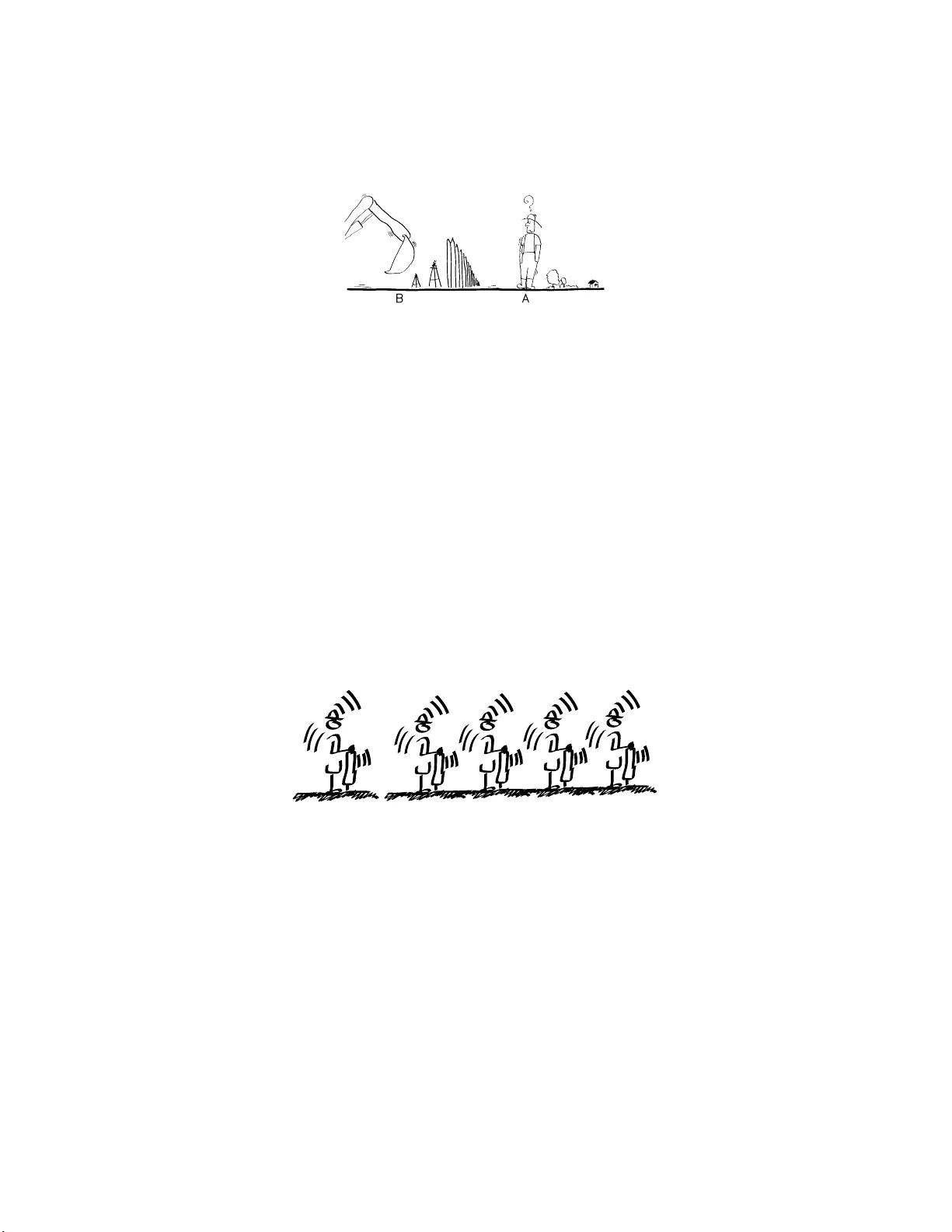
Relativ e Exp ected Improv emen t in Krigi n g Bas ed Optimization Luk asz Laniewski-W o l lk Institute of A er onautics and Applie d Me chan ics W arsaw Univ ersity o f T ec hnology No w owie jsk a 24, 0 0-665 W arsa w, P oland e-mail: llaniewski@meil.p w.edu.pl W eb page: h ttp://c-cfd.meil.p w.edu.pl/ F ebruary 4, 2020 Abstract W e prop ose an exten sion of th e concept of Exp ected I mprov ement criterion commonly u sed in Kriging based optimization. W e extend it for more complex Kriging mo dels, e.g. mo dels using deriv atives. The target field of application are CFD problems, where ob jectiv e function are extremely expensive to ev aluate, but the theory can b e also used in other fiel ds. 1 INTR ODUCTION Global optimization is a common task in adva nced engineering. The ob- jectiv e function can b e very exp ensive to cal culate or measure. In par- ticular t h is is t he case in Computational Fluid D ynamics (CFD) w here sim ulations are extremely expensive and t ime-consuming. A t present, the CFD cod e can also generate the exact deriv atives of the ob jective function so we can use them in our mo dels. The long compu tation t o ev aluate the ob jective function and (as a rule) high dimension o f the design space mak e the optimization p rocess very time-consuming. Widely adopted strategy for s uch o b jectiv e functions is to use response function meth o dology . I t is based on constructing an app ro ximation o f the ob jective function based on so me measurements and su b sequently finding p oints of new measurements that enhance our knowledge ab out the lo cation of optimum. One of t he commonly used response fun ctions mod els is the K riging mod el [2, 4, 5, 3]. This statistical estimation model considers the ob jec- tive function to be a realization of a random field. W e can construct a least squ are estimator. If we assume t h e field to b e gaussian, the least square estimator is the Ba yesian estimator. Conditional distribution of 1 the field with respect to the measuremen ts ( a p osteriori ) is also gaussian with known b oth m ean and co v ariance. One of t he method s to fi nd a p oint for n ew measurement is the Ex- p ected Imp ro vemen t criterion[3]. It uses a Ex p ected Improv emen t func- tion: EI( x ) = E (min ( ˆ F min , F ( x ))) where F is the a p osteriori field and ˆ F min is the minimum of estimator. The new p oint of measurement is chosen in the minim um of EI function. Man y mod ifi cations and enhancements w ere considered for the Kriging mod el. Application of linear op erators, e .g. deriv ativ es, integral s and conv olutions, are easy to incorp orate in the mo del[4 , 5]. Eac h of these exten sions of classic Kriging mo del is based on measuring something else th en is returned as the resp onse. F or example we measure gradien t and val ue of the function, but the resp onse is only the function. The Exp ected Improv ement states that we should measure the function in place where the minim um of resp onse can b e mostly improv ed. But for classic mod el the notion of the measured and the resp onse functions are the same. The purp ose of t his p ap er is th e investi gation w ether th e concept of EI can b e extend ed for enhanced Kriging mo dels. 2 RELA TIVE EXPECTED IMPR O VE- MENT 2.1 Efficien t Global Optimization Jones et al.[3] prop ose an Efficient Global Optimization (EGO) algorithm based on Kriging mo del and Exp ected Impro vement. It consists of the follo wing steps: 1. S elect a learning group x 1 , . . . , x n . Measure ob jective function f in these p oints f i = f ( x i ). 2. Construct a Kriging appro ximation ˆ F based on meas urements f 1 , . . . , f n . 3. Find t h e minimum of EI( x ) function for the approximation. 4. A ugment n and set x n at th e minimum of EI. 5. Measure f n = f ( x n ) and go back to 2 EI function can hav e many local minima (is highly multi-modal) and is p otential ly hard to minimize. The original paper prop osed Br anch and Bound Algorithm (BBA) to efficien tly optimize the EI function. T o use BBA auth ors h ad to establish upp er and low er bond s on minimum of EI function ov er a region. It w as fairly easy and was the main source of effectiveness of EGO. While prop osing an extension of EI concept w e also hav e to p rop ose a suitable metho ds of it’s optimization. 2.2 Gaussian Kriging Kriging, is a statistical metho d of app ro ximation a multi-dimensional function basing on va lues in a set of p oints. The Kriging estimator (ap- 2 proximati on) can b e interpreted as a least-square estimator, bu t also as a Bay es estimator. W e will use the latter interpretation as in th e original EI definition. Let us take an ob jective function f : Ω → R . F or some probabilistic space (Γ , F , P ) , w e consider a random gaussian field F on Ω with the known mean µ and co v ariance K ( x, y ). Now we take a measurements of the ob jectiv e at points x 1 , . . . , x n as f i = f ( x i ). The Bay es estimator of f is: ˆ F ( x ) = E ( F ( x ) | ∀ i F ( x i ) = f i ) Where E ( A | B ) is co nditional e xp ected v alue of A with respect to B . This estimator at y will b e called the resp onse at y and the ( x i , f i ) pairs will b e called measurements at x i . Let us take a n even t M = {∀ i F ( x i ) = f i } ⊂ Γ and a a p osteriori probabilit y space ( M , F M , P ( · | M )). E M will stand for exp ected v alue in a p osteriori . Field F considered on the M space is also a gaussian random field with kno wn b oth mean µ M and cov ariance K M . W e will call this field, the a p osteriori field. 2.3 F rom EI t o REI W e would w an t to estimate how much the minimum of ˆ F w e will be impro ved if will measure f at some p oint. Estimator ˆ F after the mea- surement in x can b e writhen as F x = E M ( F | F ( x )). The b est estimate of the effect would be E M inf Ω F x . But computing it w ould b e very time- consuming. The idea of Exp ected I mprov ement (EI) is to tak e EI( x ) = E M min { F min , F ( x ) } where F min is the actual minimum of approximation ˆ F . Exp ected Im- prov ement is in fact exp ected v alue of how resp onse at x will improv e the actual minimum of ˆ F . Of course the defin ition is equiv alent to: EI( x ) = E M min { F min , E M ( F ( x ) | F ( x ) ) } This formulati on has a natu ral extension. Let us d efine, for a set of p oints η = { η 1 , . . . , η l } , a augmen ted estimator F η ( x ) = E M ( F ( x ) | F ( η 1 ) , . . . , F ( η l )). F or another set of p oints ζ = { ζ 1 , . . . , ζ k } w e can define: REI( ζ , η ) = E M min { F min , F η ( ζ 1 ) , . . . , F η ( ζ k ) } Our Relativ e Exp ected Improv emen t (REI) is the exp ected val ue of how muc h the response at ζ will improv e the minimum of ˆ F if we measure at η . This definition implies R EI( { x } , { x } ) = EI( x ). W e can use also a more general versi on: REI m ( ζ , η ) = E M min { F η ( ζ 1 ) , . . . , F η ( ζ k ) } The main advan tage of R EI function is that w e can examine the re- sp on se in a different region th en t he region of acceptable measuremen ts. A simple example illustrates it very w ell: 3 Figure 1: A and B sets of p ossible drilling p oints Example 1 We’ r e se ar ching f or some miner al. We have to estimate the maximum miner al c ontent i n someb o dy’s land b ef or e buying it. We c annot dril l at his estate, but we c an dril l everywhe r e ar ound it. In this example resp onse an d measurements are in a different regions, so w e cannot use EI. If the estate is A and the su rroun ding ground is B , in order to find the b est place to drill, w e would hav e to search for the minim um of REI( { x } , { y } ) for x ∈ A and y ∈ B . 3 APPLICA TION 3.1 P opulations of measuremen t p oin ts The first application of using R EI in stead of EI is when we wan t to find a collection of measurement p oints instead of a single p oin t, e.g. when the ob jective function can b e compu ted sim ultaneously at these p oints . It’s a p ossibilit y of making th e optimization p ro cess more parallel. (a) (b) Figure 2: (a) One p oint of measur ement. (b) Population of meas ur ement po ints. Example 2 We have k pr o c essors to solve our CFD pr oblem, e ach run- ning a sep ar ate flow c ase. This p rocedu re could b e, for examp le, to optimize REI( { ζ 1 , . . . , ζ n } , { ζ 1 , . . . , ζ n } ). The main adv antage in u sing such an expression, ov er using some selection of EI minima, is that REI considers the correlation b etw een these p oints . F or example, if x and y are strongly correlated, we don’t wan t to measure in b oth these p oints, b ecause the v alue in x implies th e v alue in y . 4 3.2 Input enhancemen ts The other app lication fi eld is enh ancing the Kriging mo del, by some other accessible information th an the v alues in points. Let us d efine a g eneralized p oint as a pair ( x, P ), where x ∈ Ω is a p oint, and P is a linear op erator. W e can say that f ( x , P ) = ( P f )( x ). The field F ( x, P ) is also gaussian with: µ ( x, P ) = ( P µ )( x ) K ( x, P ; y , S ) = P x S y K ( x, y ) where P x stands for applying P to K as a function of the first co efficien t. Now all the earlier definitions can be extended to generalized p oints. (In fact this enhancement can be done by enlarging Ω to Ω × { Id , P, S, . . . } ) Example 3 The CFD c o de is solving the main and the adjoint pr oblem. We have b oth the value of our obje ctive and i ts derivatives with r esp e ct to design p ar ameters. We want to find the b est plac e to m e asur e these values. W e can u se f ( x , ∂ ∂ x k ) = ∂ f ∂ x k ( x ) to interpret measuring t h e d eriv atives of f interpret as measuring at p oints ( x , ∂ ∂ x k ). In th e examp le w e hav e not only calculated the v alue at ( x, Id), but also at ( x, ∂ ∂ x k ). If w e hav e d design parameters (that is Ω ⊂ R d ) w e hav e d + 1 measuremen ts sim ultaneously . W e can now optimize: REI „ ( ζ 1 , Id) , . . . , ( ζ d +1 , Id) ff ,  ( x, Id) , ( x, ∂ ∂ x 1 ) , . . . , ( x , ∂ ∂ x d ) ff« W e take d + 1 points of response ζ to maximize the effect of all t he mea- sured d eriv atives. W e could of course use EI. In that case we w ould select the n ext p oin t as if we’re measuring only the v alue. By using REI we’re incorporating the deriv ativ e information not only in the mo del, but also in t he selection process. The disadv antage of such an expression is that w e searc h in Ω d +2 whic h is d · ( d + 2)-dimensional. 3.3 Multi-effect resp onse Next on our list is the multi-effect mod el. W e can imagine that our mea- sured function is comp osed of several indep end ent or dep endent effects, while our ob jective function is only one of t h em. The simplest case is when w e w ant to optimize ob jective which w e measuring with an unknown error. Let us now say that F consists of sev eral comp onents F ( x ) = ( Z ( x ) , W ( x ) , V ( x ) , . . . ). Same letters will stand for linear operators, suc h that F ( x, Z ) = Z ( x ). Example 4 Supp ose that we’r e se ar chi ng for miner al A , but our dril ling e quipment f or m e asuring c ontent of A , c annot distinguish it fr om another miner al B . W e know on the other hand that the latter is distribute d r an- domly and in smal l p atches. Let Z b e our ob jective function (mineral A con ten t) and ε a spatiall y- correlated error (mineral B conten t). W e can measure only Z + ε while we w an t to optimize Z . In this ex ample we can optimize REI( { ( x, Z ) } , { ( x, Z + 5 ε ) } ). Such a proced u re will sim ultaneously take into consideration opti- mization of the ob jective and correction of the error. T o fully understand why this ex ample is imp ortant, w e hav e to remember that d rilling in th e same place t wice wo uld give the same result. The error correction in our proced ure will b ear this in mind and will av oid d uplication of measure- ments. This mo del w ould include results obtained from lo wer-quality numer- ical calculations. F or an iterativ e algorithm (n on-random), we can state a higher erro r bound and reduce the number o f iterations. W e cannot assume the error to be fully random, b ecause starting from the same p a- rameters, the algo rithm will give th e s ame results. That’s wh y a go o d Kriging mod el, wo uld recognize the error to b e a narro wly correlated ran- dom field ε . (a) (b) Figure 3: (a) High and (b) low fidelity mo dels Example 5 We have two CFD mo dels. O ne ac cur ate and the other ap- pr oximate, but very f ast (hi gh and low-fidelity mod els). We know also, that the l ow-fidelity mo del i s “smo othe” wi th r esp e ct to the design p ar ameters. Let Z b e our ob jective function and W b e a approximation of Z . In this example we can separately optimize: REI( { ( ζ 1 , Z ) , . . . , ( ζ k , Z ) } , { ( x, Z ) } ) REI( { ( ζ 1 , Z ) , . . . , ( ζ k , Z ) } , { ( x, W ) } ) and subsequently c hoose b etw een these tw o p oin ts. Field W is strongly spatially-correlated (“smooth”) and as suc h it’s measurement can h a ve wider effect than Z . W e can also take in to consideration the cost of the computation and select a better impr ovement-to-c ost ratio. 3.4 Robust resp onse The last field of application, that we will d iscus, is the robust resp onse. If for instance after optimization, the optimal solution will b e used to manufa cture some ob jects, we can b e sure that the ob ject will be manu- factured within certain tolerance. In oth er words, if the selected p oin t is x , th e actual p oint will b e x + ǫ . Our real ob jective function is the av erage p erformance of th ese x + ǫ . 6 (a) (b) Figure 4: (a) Desig ned and (b) manuf actured pro duct Example 6 Supp ose we c an c al culate the dr ag f or c e of a c ar. Our f actory, makes c ars with some known ac cur acy. W e want to find the c ar shap e, that wil l give the lowest aver age dr ag when made in our f actory. Let Z b e our ob jective function and ǫ - the manufacturing error. W e can measure on ly Z ( x ) while we w an t to optimize E Z ( x + ǫ ). Let us sa y that ǫ is a random v ariable (for instance N (0 , Σ)), and let φ ǫ b e it’s probabilit y density . No w E ( h ( x + ǫ )) = ( φ ǫ ∗ h )( x ) = h ( x, φ ǫ ∗ ). In ab o ve example we can use: REI ( { ( ζ , φ ǫ ∗ Z ) } , { ( η , Z ) } ) The robust resp onse stated as above , has a goo d physical in terpretation. It is also fairly easy to use as long as we can effectively calculate con vo lution of φ ǫ and the cov ariance function. It’s also go od to look at this kind of robust resp onse, as a p enalt y for the second deriv ativ e. If ǫ ∼ N (0 , Σ), th en: E ( h ( x + ǫ )) ≃ h ( x ) + 1 2 X ij ∂ 2 h ∂ x i ∂ x j Σ ij Of course such a p enalty w ould also b e a linear op erator P Σ h = h + 1 2 P ij ∂ 2 h ∂ x i ∂ x j Σ ij and as such can b e used instead of φ ǫ ∗ . This approac h can b e useful for convo lutions that are exp en sive to calculate. 4 OPTIMIZA TION 4.1 Upp er b ounds As Jones et al.[3] noted, EI funct ion can b e h ighly multi-mo d al and p oten- tially hard to optimize. T o use the branch and b ound algorithm (BBA), w e hav e to establish a goo d upp er b ound s on R EI . W e d efined REI to b e: REI( ζ , η ) = E M min { F min , F η ( ζ 1 ) , . . . , F η ( ζ k ) } where F η ( x ) = E M ( F ( x ) | F ( η 1 ) , . . . , F ( η l )). It is clear t h at F η is a gaussian field (in fact with only l degrees of freedom). W e can calculate 7 its mean an d cov ariance dep ending on η . I n such a case w e w ould wan’t to establish up p er b ounds for an expresion: Ψ µ, Σ = E min { γ 1 , . . . , γ p } for some γ ∼ N ( µ, Σ). T o b ound such an expression, we can use re- cent ext ensions of comparison p rinciple by Vitale[7]. The comparison principle states that the Φ µ, Σ is greater, the grea ter ar e E ( γ i − γ j ) 2 = Σ ii + Σ j j − 2Σ ij . T o calculate the u pp er b oun d for REI, w e can maximize these expressio ns o ver a region and then calculate t h e indep endent but differently distri buted (IDD) gaussia n v ariables dominating REI . Con- struction of such d ominating IDD v ariables is discussed in R oss[6]. 4.2 Exact calculation In th e last iterations of BBA the IDD - based b ounds will b e insufficient. The main direction of further research will b e to establish a goo d metho d of calculating an exact b ound on Ψ µ, Σ . Actual algorithms in this fi eld are based on Monte Carlo or quasi-Monte Carlo m eth od s, for instance using results by Genz[1]. 5 CONCLUSIONS Relative Exp ected Improv emen t is prop osed to extend the concep t of E I for more complex Kriging models. It can help searc h for new points of measuremen ts and for p opu lations of such p oin ts. It can also help to use deriv ative information more efficiently . F urther research is needed to find efficien t implementation of this concept. 6 A CKNO WLEDGEMENTS This work was supp orted by FP7 FLOWHEAD pro ject (Fluid Op timisa- tion W orkflows for Highly Effective A utomotive D evelo pment Pro cesses). Gran t agreement no.: 218626. I would also like t o thank p rofessor Jacek Rokicki from the I n stitute of Aeronautics and Applied Mechanics (W arsa w U niversit y of T ec h n ology) for encouragement and help in scientific researc h. References [1] Alan Genz. N umerical compu tation of multiv ariate normal probab il- ities. Journal of Computational and Gr aphic al St atistics , 1:1 41–150, 1992. [2] T ob y J. Mitchell Jerome Sacks, William J. W elc h and Hen ry P . Wynn. Design and analysis of comput er exp eriments. Statistic al Scienc e , 4(4):409–4 23, Nov ember 1989. 8 [3] Donald R. Jones, Matth ias Schonlau, and William J. W elch. Efficien t global optimization of exp ensive black-box functions. Journal of Glob al Optimization , 13(4):455–49 2, December 1998. [4] Stephen J. Leary , Atul Bhask ar, and Andy J. Keane. A deriv ative based surrogate mo d el for approximating and optimizing the outp ut of an exp ensive computer sim ulation. Journal of Gl ob al O ptim ization , 30(1):39–5 8, September 2004. [5] T ob y J. Mitchell Max D . Morris and Donald Ylvisaker. Ba yesian design and analysis o f computer exp eriments: Use of deriv atives in surface prediction. T e chnometrics , 35(3):455–492 , Au gust 1993. [6] Andrew M. Ross . Computing b ounds o n th e exp ected maximum of correlated n ormal v ariables. Metho dolo gy and Computing in App lie d Pr ob abil ity . [7] Richard A. Vitale. Some comparisons for gaussian pro cesses. Pr o c e e d- ings of the Americ an Mathematic al So ci ety , 128:3043 , 2000. 9