Subspace Pursuit for Compressive Sensing Signal Reconstruction

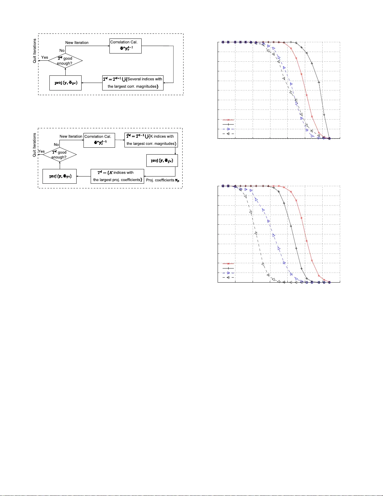
1 Subspace Pursuit for Compressi v e Se nsing Signal Reconstruction W ei Dai a nd Olgica Milenkovic Department o f Electrical and Compu ter Engineering Univ ersity of Illinois at Urba na-Champaign Abstract —W e propose a new method for reconstruction of sparse signals with and without noisy perturbations, termed the subspace pu rsuit algorithm. The algorithm has two important characteristics: low computation al complexity , comparable t o that of orthogonal matching pursuit techniques when applied to v ery sparse signals, and reconstruction accuracy of the same order as that of LP optimization method s. Th e presented analysis shows that in the n oiseless settin g, the proposed algorithm can exactly reconstruct arbitrary sparse signals provided that the sensing ma trix sa tisfies the restricted i sometry property with a constant parameter . In the noisy setting and in the case that the signal is not exa ctly sp arse, it can be shown that the mean squared err or of the reconstruction is u pper bounded by constant multiples of the measureme nt and signal perturbation energies. Index T erms —Compressi ve sensing, orthogonal matching pur- suit, reconstruction algorithms, restricted isometry p roperty , sparse signal r econstruction. I . I N T R O D U C T I O N Compressive sensing (CS) is a samp ling method closely connected to transform co ding which has been widely used in moder n co mmunication systems in volving large scale data samples. A transform co de converts input signals, embedded in a high dimen sional space, into signals that lie in a space of significan tly smaller dimension s. Examples of transform coders include the well known wavelet transforms and the ubiquito us Fourier tran sform. Compressive sensing techniqu es per form tran sform cod- ing suc cessfully whenever applied to so-called compr essible and/or K -sparse signals, i.e., signals that can be represented by K ≪ N significant coe ffi cients over an N -dimension al basis. Encodin g of a K -sparse, discrete-time signal x o f dimension N is accomp lished by com puting a measuremen t vector y that consists of m ≪ N linear pr ojections of the vector x . This can be co mpactly d escribed via y = Φx . Here, Φ r epresents an m × N matrix, usually o ver the field of re al n umbers. Wit hin this fra mew ork, the projection basis is assumed to b e incoherent with the basis in which the signal has a spar se rep resentation [ 1]. Although the reconstructio n of th e sign al x ∈ R N from the possibly noisy random pr ojections is an ill-po sed problem, th e This work is supported by NSF Grant s CCF 0644427, 0729216 and the D ARP A Y oung Facult y A ward of the second author . W ei Dai and Olgica Mil enko vic are with the Department of Elec trical and Computer Enginee ring, Univ ersity of Ill inois at Urbana-Cha mpaign, U rbana, IL 61801-2 918 USA (e-mail : weidai07@ uiuc.edu; milenk ov@u iuc.edu). strong prior kn owledge of signal sparsity allows for recovering x using m ≪ N projection s only . One o f the outstanding results in CS theory is that the signal x can b e reconstructed using optim ization strategies aimed at finding the sparsest signal tha t matches with the m p rojections. In other words, the reconstruction p roblem c an b e cast as an l 0 minimization problem [2]. It can be shown that to reconstruct a K -spar se signal x , l 0 minimization r equires only m = 2 K rand om pro- jections wh en the sign al and the measurem ents are noise-fre e. Unfortu nately , the l 0 optimization pro blem is NP-hard . This issue has led to a large body o f work in CS theory and practice centered arou nd the d esign of measurement and re construction algorithm s with tractable rec onstruction co mplexity . The work by Do noho and Candès et. al. [1], [3], [4], [5] demonstra ted that CS reconstru ction is, in deed, a polynom ial time p roblem – albeit under the constraint that more than 2 K measuremen ts ar e used. The key o bservation beh ind th ese findings is that it is not necessary to re sort to l 0 optimization to recover x from the un der-determined in verse prob lem; a much easier l 1 optimization , based on Linear Programm ing (LP) techniques, yields an equiv alent solution , as long as the sampling matrix Φ satisfies the so called r estricted isometry pr operty (RIP) with a con stant pa rameter . While L P techniques play an impor tant role in designing computatio nally tractab le CS decoders, their com plexity is still highly impr actical f or many applications. I n su ch cases, the need f or faster decod ing algorith ms - prefer ably operating in linear time - is of critical importance, even if one has to increase the numb er of m easurements. Several classes of low-complexity reconstru ction techn iques were recently put forward as altern ati ves to lin ear prog ramming ( LP) based recovery , which include group testing m ethods [ 6], an d al- gorithms based on belief propagation [7]. Recently , a family of iterati ve greedy algor ithms received significant attention due to their low complexity and simple geometric in terpretation. They includ e the Ortho gonal Match- ing Pursuit (OMP), th e Regularized OMP (ROMP) an d the Stagewise OMP (StOMP) algorithms. The ba sic idea b ehind these methods is to find the sup port o f the unkn own signal sequentially . At each iteration of the algorithms, one or several coordin ates of the vector x are selecte d for testing based on the correlation values between th e co lumns o f Φ an d the regularized measurement vector . If deem ed suf ficiently reliable, the c andidate column ind ices ar e sub sequently ad ded to the curren t estimate of the su pport set of x . The pursuit algorithm s iterate this pr ocedure u ntil all th e c oordinate s in 2 the correct sup port set ar e in cluded in th e estimated sup port set. The computation al com plexity of OMP strategies depends on the number of iterations needed for exact r econstruction : standard OMP always run s throu gh K iterations, and ther e- fore its re construction complexity is rough ly O ( K mN ) (see Section IV -C fo r details). This co mplexity is sign ificantly smaller than that o f LP m ethods, especially when the signal sparsity le vel K is small. Ho wever , the pursuit alg orithms do not h a ve p rovable recon struction quality at the le vel of LP methods. For OMP techn iques to oper ate successfully , one requires that the correlation b etween all p airs o f colu mns of Φ is at most 1 / 2 K [8], which b y the Gershgorin Circle Theorem [9] represen ts a mo re restricti ve c onstraint than the RIP . T he R OMP algor ithm [10] can r econstruct all K - sparse signals provid ed that the RIP holds with pa rameter δ 2 K ≤ 0 . 06 / √ log K , which streng thens the RIP requirem ents for l 1 -linear programm ing b y a factor of √ log K . The main contribution of this paper is a new algo rithm, termed the sub space pursuit (SP) algorithm. It has provable reconstruc tion capability comparable to that of LP metho ds, and exhibits th e low reco nstruction co mplexity of match ing pursuit techniques for very sparse signals. The algorithm can operate both in the noiseless and noisy regime, allowing for exact and appr oximate signal recovery , r espectiv ely . F or any sampling matrix Φ satisfying the RIP with a constant parameter in depende nt of K , the SP algorithm can recover arbitrary K -sparse signals exactly f rom its noiseless mea- surements. When the measur ements are inaccurate an d/or the signal is no t exactly spar se, th e rec onstruction distortio n is upper boun ded by a constant multiple of the measu rement and/or signal perturbatio n energy . For very sparse signals with K ≤ con st · √ N , which, fo r example, ar ise in certain commun ication scenarios, the comp utational complexity of the SP algor ithm is upp er bounded by O ( mN K ) , but can b e further redu ced to O ( mN log K ) when the no nzero entries of the spar se signal decay slo wly . The basic idea behin d the SP algorithm is borrowed from coding th eory , more p recisely , th e A ∗ order-statistic algo - rithm [ 11] for additive wh ite Gau ssian noise chann els. In this d ecoding framework, one starts by selecting the set of K mo st r eliable in formation sym bols. T his highest reliab ility informa tion set is subseque ntly hard-decision decoded, and the metric of the parity checks correspon ding to the given informa tion set is evaluated. Based on the v alue of th is metric, some of the low-reliability symbols in the most reliable informa tion set are changed in a sequ ential ma nner . The algorithm can therefo re be seen as op erating on an adaptiv ely modified coding tree. If th e no tion of “most r eliable sym bol” is replaced by “colu mn of sensing matrix exhibiting highest correlation with the vector y ”, the notion of “parity-ch eck metric” by “residual metric”, then the above method c an be easily changed fo r use in CS reconstru ction. Consequ ently , one c an per form CS reconstruction by selecting a set of K columns of the sensing matrix with highest corr elation that span a can didate subspace for the sen sed vector . If the distance of the receiv ed vector to this space is deemed large, the algorithm increm entally removes and adds ne w basis v ectors accordin g to their reliability values, un til a sufficiently clo se candidate word is identified . SP emp loys a search strategy in which a consta nt number of vectors is expu rgated f rom the candidate list. This featur e is main ly introdu ced for simplicity of an alysis: one can easily extend the algorith m to include adaptive expu rgation strategies that do not necessarily o perate on fixed-sized lists. In com pressiv e sensing, the major challeng e associated with sparse signal recon struction is to identify in which subspace, generated by no t mor e than K columns of the matrix Φ , the measured signal y lies. On ce the correct subspace is determined , the no n-zero signa l coefficients are calculated b y applying the p seudoinversion pro cess. The defining char acter of the SP algorithm is the metho d used for finding the K columns that spa n th e c orrect su bspace: SP tests subsets of K columns in a g roup, for the purpose of refining at each stage an initially chosen estimate fo r the subspace. More specifically , the algor ithm maintains a list of K columns o f Φ , perfor ms a simple test in the sp anned spa ce, an d the n refines the list. If y does not lie in the curre nt estimate fo r the co rrect spanning space, one refines the estimate by retaining reliable candidates, discarding the unreliable ones wh ile add ing the same n umber of new candidates. T he “reliability proper ty” is captured in terms of th e order statist ics of the inn er p roducts of the receiv ed signal with the colu mns of Φ , and the sub space projection co efficients. As a conseque nce, the main d ifference b etween R OMP a nd the SP recon struction strategy is that the for mer algorithm generates a list o f candidates sequen tially , witho ut bac k- tracing: it starts with a n empty lis t, identifies one or se veral reliable candidates during e ach iteration, and adds them to the already existing list. Once a coord inate is d eemed to be reliable and is add ed to the list, it is not removed from it until the algo rithm term inates. Th is search strategy is overly restrictiv e, since candidates have to be selected with e xtreme caution. I n con trast, the SP alg orithm inco rporates a simple method for re-ev aluating th e reliability of all candidates at each iteration of the process. At the time of writing this m anuscript, th e auth ors becam e aware o f the related work by J. Tropp, D. Needell and R. V er - shynin [12], describ ing a similar recon struction algorithm. The main d ifference between the SP algorithm and the CoSAMP algorithm of [1 2] is in the man ner in which new candidates are added to the list. In each iteration, in the SP algorithm, only K new ca ndidates are add ed, while the CoSAMP algor ithm adds 2 K vecto rs. This m akes the SP alg orithm comp utationally more efficient, but the un derlying analy sis more com plex. In addition, the restricted isometry con stant fo r which the SP algorithm is gu aranteed to converge is larger than the one presented in [12]. Finally , this paper also contains an analysis of the n umber of iter ations neede d for reconstructio n of a sparse signal (see Theore m 6 for deta ils), fo r which ther e is no counterpart in the CoSAMP study . The r emainder of the p aper is organized as fo llows. Sec- tion II intro duces relev ant concepts and termino logy for de- scribing the proposed CS r econstruction technique. Sec tion III contains the algo rithmic description of the SP algo rithm, along with a simulation-b ased stud y of its perform ance when com - pared with OMP , R OMP , and LP meth ods. Section IV contain s 3 the main result o f the paper pertaining to th e noiseless setting: a fo rmal pro of for th e guaran teed reconstruc tion per forman ce and the reconstruction complexity of the SP algorithm. Sec- tion V con tains the main result of th e paper pertain ing to the noisy setting . Conclu ding remarks are gi ven in Section VI, while proofs of most of the theo rems a re presented in the Append ix o f the pap er . I I . P R E L I M I N A R I E S A. Compress ive Sen sing and the Restricted Isometry Pr operty Let supp ( x ) de note the set of indices of the non -zero coordin ates of an arbitr ary vector x = ( x 1 , . . . , x N ) , and let | supp ( x ) | = k · k 0 denote th e suppor t size of x , or equivalently , its l 0 norm 1 . Assume next that x ∈ R N is an u nknown sign al with | supp ( x ) | ≤ K , and let y ∈ R m be an observation o f x via M linear m easurements, i.e., y = Φx , where Φ ∈ R m × N is he nceforth r eferred to as the samplin g matrix . W e are concerned with the problem of low-complexity recovery of the unknown signal x from the me asurement y . A natural formu lation of the recovery proble m is within an l 0 norm minimization framework, which seeks a solution to the problem min k x k 0 sub ject to y = Φx . Unfortu nately , the above l 0 minimization pro blem is NP-hard, and hence can not be used for practical application s [3], [4]. One way to a void using this computationally intractable for- mulation is to co nsider a l 1 -regularized optimization p roblem, min k x k 1 sub ject to y = Φx , where k x k 1 = N X i =1 | x i | denotes the l 1 norm of th e vector x . The main advantage of the l 1 minimization approa ch is th at it is a conv ex optimization problem that can be solved e ffi - ciently by lin ear progr amming (LP) techniqu es. Th is method is theref ore f requently referr ed to as l 1 -LP recon struction [3], [13], and its reconstruction complexity equals O  m 2 N 3 / 2  when interior po int methods are employed [14]. See [15], [16], [17] fo r othe r metho ds to further red uce the comp lexity o f l 1 - LP . The reconstruction accur acy of th e l 1 -LP method is de- scribed in terms of th e r estricted isometry pr o perty (RIP) , formally defined below . Definition 1 (T runcation): Let Φ ∈ R m × N , x ∈ R N and I ⊂ { 1 , · · · , N } . The matrix Φ I consists of the colu mns of Φ with indices i ∈ I , and x I is c omposed of the entries of x indexed by i ∈ I . Th e space spanned by the columns of Φ I is d enoted by span ( Φ I ) . Definition 2 (R IP): A m atrix Φ ∈ R m × N is said to satisfy the Restricted I sometry Pro perty (RIP) with parameter s ( K, δ ) 1 W e interchan geably use both notations in the paper . for K ≤ m , 0 ≤ δ ≤ 1 , if for all index sets I ⊂ { 1 , · · · , N } such that | I | ≤ K and for all q ∈ R | I | , one h as (1 − δ ) k q k 2 2 ≤ k Φ I q k 2 2 ≤ (1 + δ ) k q k 2 2 . W e define δ K , the RIP constant, as the infimu m of a ll parameters δ for which the RIP holds, i.e. δ K := inf n δ : (1 − δ ) k q k 2 2 ≤ k Φ I q k 2 2 ≤ (1 + δ ) k q k 2 2 , ∀ | I | ≤ K, ∀ q ∈ R | I | o . Remark 1 (R IP and eigen values): If a sampling m atrix Φ ∈ R m × N satisfies the RIP with parameters ( K, δ K ) , then for all I ⊂ { 1 , · · · , N } such that | I | ≤ K , it holds th at 1 − δ K ≤ λ min ( Φ ∗ I Φ I ) ≤ λ max ( Φ ∗ I Φ I ) ≤ 1 + δ K , where λ min ( Φ ∗ I Φ I ) and λ max ( Φ ∗ I Φ I ) denote the minimal and maximal eigenv alues of Φ ∗ I Φ I , respectiv ely . Remark 2 (Ma trices satisfying the RIP): Most known f am- ilies of matrices satisfying the RIP p roperty with op timal or near-optimal perform ance gu arantees are ran dom. Examples include: 1) Random matrices with i.i.d. entries that follo w either the Gaussian distribution, Bernoulli d istribution with zero mean and variance 1 /n , or any other distribution that satisfies certain tail decay laws. It was shown in [13] that the RIP for a rand omly ch osen m atrix from such ensembles holds with overwhelmin g prob ability whenever K ≤ C m log ( N/ m ) , where C is a func tion of the RIP con stant. 2) Random matrices fro m the Fourier ensemble. Here, one selects m rows from the N × N discrete Four ier transform matrix un iformly a t rando m. U pon selection, the co lumns of the matrix are scaled to unit norm. The resulting matrix satisfies the RIP with overwhelming probab ility , provid ed that K ≤ C m (log N ) 6 , where C depends o nly on the RIP constant. There exists an intimate conne ction between the L P reco n- struction accuracy and the RIP pro perty , first described by Candés a nd T ao in [3]. If the sampling matrix Φ satisfies the RIP with co nstants δ K , δ 2 K , and δ 3 K , such that δ K + δ 2 K + δ 3 K < 1 , (1) then the l 1 -LP algorithm will recon struct all K - sparse signals exactly . This sufficient cond ition (1) can be im proved to δ 2 K < √ 2 − 1 , (2) as demonstrated in [18]. For s ubseque nt deriv ations, we need tw o results summarized in th e lemm as below . The first part of th e claim, as well as a related modificatio n of the second c laim also app eared in [3 ], [10]. For comp leteness, we in clude the p roof of the lemma in Append ix A. 4 Lemma 1 (Con sequences o f the RIP): 1) (Monoton icity o f δ K ) For any two integers K ≤ K ′ , δ K ≤ δ K ′ . 2) (Near-orthogonality of colu mn s) Let I , J ⊂ { 1 , · · · , N } be two d isjoint sets, I T J = φ . Sup pose that δ | I | + | J | < 1 . F or arbitrary vectors a ∈ R | I | and b ∈ R | J | , |h Φ I a , Φ J b i| ≤ δ | I | + | J | k a k 2 k b k 2 , and k Φ ∗ I Φ J b k 2 ≤ δ | I | + | J | k b k 2 . The lemma imp lies that δ K ≤ δ 2 K ≤ δ 3 K , which con se- quently simplifies (1) to δ 3 K < 1 / 3 . Both (1) and (2) rep resent sufficient conditio ns for exact recon struction. In o rder to describe the m ain steps of the SP algorithm, we introdu ce next the notion of the p rojection of a vector an d its residue. Definition 3 (P r o jection an d Resid u e): Let y ∈ R m and Φ I ∈ R m ×| I | . Suppose that Φ ∗ I Φ I is in vertible. The projection of y onto s pan ( Φ I ) is d efined as y p = pr o j ( y , Φ I ) := Φ I Φ † I y , where Φ † I := ( Φ ∗ I Φ I ) − 1 Φ ∗ I denotes the pseud o-inv erse of the matrix Φ I , a nd ∗ stands fo r matrix transposition. The r esidu e vector of th e projection equals y r = resid ( y , Φ I ) := y − y p . W e find th e fo llowing prope rties of p rojections and r esidues of vectors useful for o ur subseq uent der i vations. Lemma 2 (Pr ojection and Residu e): 1) (Orthogonality of the r esidue) For an arb itrary vector y ∈ R m , and a sampling matrix Φ I ∈ R m × K of full column rank, let y r = r esid ( y , Φ I ) . Then Φ ∗ I y r = 0 . 2) (Appr oximation of the pr o jection r esidue) Consider a matrix Φ ∈ R m × N . Let I , J ⊂ { 1 , · · · N } be two disjoint sets, I T J = φ , and suppose that δ | I | + | J | < 1 . Furthermo re, let y ∈ span ( Φ I ) , y p = pr o j ( y , Φ J ) and y r = resid ( y , Φ J ) . Then k y p k 2 ≤ δ | I | + | J | 1 − δ max( | I | , | J | ) k y k 2 , (3) and  1 − δ | I | + | J | 1 − δ max( | I | , | J | )  k y k 2 ≤ k y r k 2 ≤ k y k 2 . (4) The proof of Lemma 2 can be found in App endix B. I I I . T H E S P A L G O R I T H M The main steps of th e SP algorithm a re summ arized below . 2 Algorithm 1 Sub space Pur suit Algo rithm Input: K , Φ , y Initialization: 1) T 0 = { K ind ices co rrespond ing to the largest m agni- tude entries in the vector Φ ∗ y } . 2) y 0 r = r esid  y , Φ ˆ T 0  . Iteration: A t th e ℓ th iteration, go th rough the following steps 1) ˜ T ℓ = T ℓ − 1 S { K indices co rrespond ing to the largest magnitud e en tries in the vector Φ ∗ y ℓ − 1 r  . 2) Set x p = Φ † ˜ T ℓ y . 3) T ℓ = { K indices c orrespon ding to the largest elements of x p } . 4) y ℓ r = resid ( y , Φ T ℓ ) . 5) If   y ℓ r   2 >   y ℓ − 1 r   2 , let T ℓ = T ℓ − 1 and quit the iteration. Output: 1) The estimated sign al ˆ x , satisfying ˆ x { 1 , ··· ,N }− T ℓ = 0 and ˆ x T ℓ = Φ † T ℓ y . A schematic diag ram of the SP alg orithm is dep icted in Fig. 1(b). For comp arison, a diagram o f OMP-type methods is p rovided in Fig. 1( a). Th e subtle, but impo rtant, differ- ence between the two schemes lies in the appro ach used to generate T ℓ , the estimate of the correct supp ort set T . In OMP strategies, during each iteration the algo rithm selects one or several indices tha t represent good partial supp ort set estimates an d then ad ds the m to T ℓ . Once an index is included in T ℓ , it remains in this set through out the remaind er of the reco nstruction pr ocess. As a result, strict in clusion rules are need ed to ensure that a significant fr action of the newly ad ded indices belong s to the correct support T . On the oth er hand, in the SP algorithm, an e stimate T ℓ of size K is maintain ed an d refined during each iteration. An in dex, which is consider ed reliable in some iteration but shown to be wrong at a later iteration, ca n be add ed to or rem oved from the estimated su pport set at any stag e of the re covery process. The expectation is that the recu rsi ve refinements of the estimate of the supp ort set will lead to subspaces with strictly decreasing distance from the measureme nt vector y . W e perfor med e xtensive co mputer simulations in o rder to compare the accu racy o f different r econstructio n algor ithms empirically . In th e compr essi ve sensing framew ork, all sparse signals are expecte d to be exactly reconstructed as lo ng as the lev el of the sparsity is b elow a certa in threshold. Howe ver , the co mputation al co mplexity to test this unifo rm recon struc- tion ability is O  N K  , which grows expon entially with K . Instead, fo r em pirical testing , we adop t the simulation strategy described in [5] which calculates th e empirical fr equ ency of 2 In Step 3) of th e SP algorithm, K indic es wit h the la rgest correla tion magnitude s are used to form T ℓ . In CoSaMP [12], 2 K s uch indices are used. This small dif ference results in dif ferent proofs associated with Step 3) and dif ferent RIP consta nts that guarant ee successful signal reco nstruction . 5 (a) Itera tions in OMP , Stage wise OMP , an d Regulari zed OMP: in ea ch iterat ion, one deci des on a re liable set of c andidat e indice s to be added into the list T ℓ − 1 ; once a candidate is added, it remains in the list until the algorit hm termina tes. (b) Iterations in the proposed S ubspace Pursuit Algorithm: a list of K can- didate s, whic h is allo wed to be updated during the iterat ions, is maintain ed. Figure 1 : Descr iption of recon struction algorithms fo r K - sparse signals: th ough b oth ap proaches loo k similar, the basic ideas behind th em are quite dif ferent. exact reconstruction for the Gaussian random matrix ensemble. The steps of the testing strategy are listed below . 1) For given values of the parameter s m and N , ch oose a signal sp arsity le vel K such that K ≤ m/ 2 ; 2) Randomly gener ate a m × N sampling matrix Φ fr om the stan dard i.i.d. Gau ssian ensemb le; 3) Select a support set T of size | T | = K u niformly at random , and generate the s parse signal vector x by either one of the following two m ethods: a) Draw the elemen ts o f the vector x restricted to T from the standard Gaussian distribution; we refer to this ty pe o f signa l a s a Gaussian signal. Or , b) set all entries of x supported on T to ones; we refer to th is ty pe o f sign al as a zer o-o ne sign al. Note th at zero -one sp arse signals are o f special interest for the co mparative study , since they repre sent a partic- ularly challenging case for OMP-type of recon struction strategies. 4) Compute the measuremen t y = Φx , a pply a recon- struction algorithm to obtain ˆ x , the estimate of x , and compare ˆ x to x ; 5) Repeat the process 500 time s for each K , an d then simulate the sam e algor ithm for different values of m and N . The improved re construction capability of the SP metho d, compare d with that o f th e OMP and R OMP algorithms, is illustrated by two examples shown in Fig. 2. Here, the signals are d rawn both accord ing to th e Gaussian and zero-on e model, and the benchmar k performa nce of the LP reconstructio n 0 10 20 30 40 50 60 70 0 0.1 0.2 0.3 0.4 0.5 0.6 0.7 0.8 0.9 1 Signal Sparsity: K Frequency of Exact Reconstruction Reconstruction Rate (500 Realizations): m=128, N=256 Linear Programming (LP) Subspace Pursuit (SP) Regularized OMP Standard OMP (a) Simulations for Gaussian sparse signals: OMP and R OMP start to fail when K ≥ 19 and when K ≥ 22 respecti vel y , ℓ 1 -LP be gins to fail when K ≥ 35 , and the SP algorit hm fai ls only when K ≥ 45 . 0 10 20 30 40 50 60 70 0 0.1 0.2 0.3 0.4 0.5 0.6 0.7 0.8 0.9 1 Signal Sparsity: K Frequency of Exact Reconstruction Reconstruction Rate (500 Realizations): m=128, N=256 Linear Programming (LP) Subspace Pursuit (SP) Regularized OMP Standard OMP (b) Simulations for ze ro-one sparse signa ls: both OMP and R OMP starts to fail when K ≥ 10 , ℓ 1 -LP begins to fail when K ≥ 35 , and the SP algo rithm fail s when K ≥ 29 . Figure 2: Simulations of the exact recovery rate: c ompared with OMPs, the SP algo rithm has significan tly larger critical sparsity . technique is plotted as well. Figure 2 d epicts the empirical frequen cy of e xact reconstruc- tion. The n umerical v alues on the x -axis d enote th e sparsity lev el K , while the numerical values on the y -axis represent the fraction of exactly recovered test signals. Of par ticular interest is th e sparsity le vel at which the r ecovery rate drops below 100% - i.e. the critical sparsity - which, when exceeded, leads to errors in the r econstruction algorithm applied to some of the sign als fro m the giv en class. The simulation results reveal that th e critical sparsity of the SP algorithm b y far e xceeds th at of the OMP and ROMP technique s, for both Gaussian an d zero-on e inputs. T he re- construction capability of the SP algorith m is comparable to that of the LP based approach : the SP a lgorithm has a slightly higher critical sparsity f or Gaussian signals, but also a slightly 6 lower critical sparsity for zero-one signals. However , the SP algorithm s significantly o utperfo rms the LP me thod when it comes to reconstru ction co mplexity . As we an alytically demonstra te in the expo sition to follow , th e reconstruction complexity of the SP algorithm for both Gaussian and zero-one sparse signals is O ( mN log K ) , whenever K ≤ O  √ N  , while the co mplexity o f LP algorithms based on in terior point methods is O  m 2 N 3 / 2  [14] in th e same asymp totic regime. I V . R E C OV E RY O F S PA R S E S I G NA L S For simplicity , we start b y analyzing the reco nstruction perfor mance of SP algor ithms applied to sparse signals in the noiseless setting. Th e tec hniques used in this con text, and the insights obtained are also applicable to the analysis of SP reconstruc tion schemes with signal or/and measurement perturb ations. Note that th rougho ut the remain der of the pape r , we use the notatio n S i ( S ∈ { D, L } , i ∈ Z + ) stacked over an inequ ality sign to ind icate that the inequality follows f rom Definition( D ) or Lemm a ( L ) i in the paper . A suf ficient co ndition for exact reco nstruction of arbitrary sparse signals is stated in the following theore m. Theor em 1 : Let x ∈ R N be a K -sparse signal, and let its correspon ding measur ement be y = Φx ∈ R m . If the sampling m atrix Φ satisfies the RIP with constan t δ 3 K < 0 . 165 , (5) then the SP algorithm is guaran teed to exactly recover x fro m y via a finite numb er of iterations. Remark 3: The requ irement on RIP constant can b e relaxed to δ 3 K < 0 . 205 , if we replace th e stopping criterion   y ℓ r   2 ≤   y ℓ − 1 r   2 with   y ℓ r   2 = 0 . T his claim is suppor ted by substituting δ 3 K < 0 . 205 into Equation (6). Howe ver , fo r simplicity of analysis, we adopt   y ℓ r   2 ≤   y ℓ − 1 r   2 for the iteration s toppin g criterion. Remark 4: In the origin al version of this m anuscript, we proved the wea ker result δ 3 K ≤ 0 . 06 . At the tim e of revision of the paper, we were given ac cess to the manu script [19] b y Needel and T ropp. Using some of the p roof techniq ues in their work, we managed to improve the re sults in Theorem 3 and therefor e the RIP constant of the origin al submission . The in- terested re ader is referred to http://arxiv .org/abs/080 3.0811v2 for the first version of the theorem. This paper contains only the proof of the stronger resu lt. This sufficient condition is p roved b y app lying Theo rems 2 and 6. The compu tational complexity is related to the n umber of iterations requ ired for exact recon struction, and is discussed at the end of Section IV -C. Before providing a detailed analysis of the re sults, let us sketch the main id eas behind the proof. W e denote by x T − T ℓ − 1 an d x T − T ℓ the residu al signals based upo n the estimates of supp ( x ) before and after the ℓ th iteration of th e SP algo rithm. Provided that the samplin g matrix Φ satisfies the RIP with constant (5), it hold s that k x T − T ℓ k 2 < k x T − T ℓ − 1 k 2 , Figure 3: After each iteration, a K -dimensiona l hype r-plane closer to y is obtained . which implies that at each iteration , the SP algorithm identifies a K -d imensional space that red uces the recon struction error of the vector x . See Fig. 3 for an illustration. This observation is f ormally stated as follows. Theor em 2 : Assume that the conditions of Theorem 1 hold . For each iteration of the SP algorithm, o ne h as k x T − T ℓ k 2 ≤ c K k x T − T ℓ − 1 k 2 , (6) and   y ℓ r   2 ≤ c K 1 − 2 δ 3 K   y ℓ − 1 r   2 <   y ℓ − 1 r   2 , (7) where c K = 2 δ 3 K (1 + δ 3 K ) (1 − δ 3 K ) 3 . (8) T o prove Theorem 2, we need to take a closer look at the operation s executed durin g each iteration of th e SP algo rithm. During one iter ation, two basic sets of com putations and compariso ns are per formed: first, given T ℓ − 1 , K addition al candidate indices f or in clusion in to the estimate of the support set a re iden tified; an d secon d, given ˜ T ℓ , K r eliable in dices ou t of the total 2 K indices a re selected to form T ℓ . In Subsections IV -A and IV -B, we provide the intuitio n fo r choosing th e se- lection rules. Now , let x T − ˜ T ℓ be the residue signa l coefficient vector correspon ding to the suppo rt set estimate ˜ T ℓ . W e h av e the f ollowing two th eorems. Theor em 3 : It holds that   x T − ˜ T ℓ   2 ≤ 2 δ 3 K (1 − δ 3 K ) 2 k x T − T ℓ − 1 k 2 . The proof of the theorem is postpon ed to Appendix D. Theor em 4 : The following inequality is valid k x T − T ℓ k 2 ≤ 1 + δ 3 K 1 − δ 3 K   x T − ˜ T ℓ   2 . The proof of the result is defer red to Appendix E. Based on Theorem s 3 and 4, one arri ves at the result claimed in Eq uation ( 6). 7 Furthermo re, accordin g to Lemmas 1 and 2, o ne h as   y ℓ r   2 = k resid ( y , Φ T ℓ ) k 2 = k resid ( Φ T − T ℓ x T − T ℓ , Φ T ℓ ) +resid ( Φ T ℓ x T ℓ , Φ T ℓ ) k 2 D 3 = k resid ( Φ T − T ℓ x T − T ℓ , Φ T ℓ ) + 0 k 2 ( 4 ) ≤ k Φ T − T ℓ x T − T ℓ k 2 ( 6 ) ≤ p 1 + δ K · c K k x T − T ℓ − 1 k 2 , (9) where the second equ ality holds by the d efinition of the residue, while (4) and (6) refer to the lab els of the in equalities used in the bound s. In addition,   y ℓ − 1 r   2 = k resid ( y , Φ T ℓ − 1 ) k 2 = k resid ( Φ T − T ℓ − 1 x T − T ℓ − 1 , Φ T ℓ − 1 ) k 2 ( 4 ) ≥ 1 − δ K − δ 2 K 1 − δ K k Φ T − T ℓ − 1 x T − T ℓ − 1 k 2 ≥ 1 − 2 δ 2 K 1 − δ K p 1 − δ K k x T − T ℓ − 1 k 2 ≥ 1 − 2 δ 2 K √ 1 − δ K k x T − T ℓ − 1 k 2 . (10) Upon co mbining (9 ) and (10), one obtains the following up per bound   y ℓ r   2 ≤ p 1 − δ 2 K 1 − 2 δ 2 K c K   y ℓ − 1 r   2 L 1 ≤ 1 1 − 2 δ 3 K c K   y ℓ − 1 r   2 . Finally , elemen tary calculatio ns sho w that when δ 3 K ≤ 0 . 165 , c K 1 − 2 δ 3 K < 1 , which completes th e pro of of Theorem 2. A. Why Does Correlation Maximizatio n W ork for th e SP Algorithm? Both in the initialization step and du ring each iteration of th e SP alg orithm, we select K ind ices that maximize the cor relations between the co lumn vectors and the resid ual measuremen t. Henceforth, this step is referred to as corr elation maximization (CM). Consider the ideal case where all colu mns of Φ are orthog onal 3 . In this scenario , the sign al coeffi cients can b e easily recovered by calcu lating th e corre lations h v i , y i - i.e., all in dices w ith non-zero magnitude are in the correct support of the sensed vector . Now a ssume th at the samp ling matrix Φ satisfies th e RIP . Recall that the RIP (see L emma 1) implies that the colum ns are locally near-orthogo nal. Con- sequently , fo r a ny j not in th e correct supp ort, the magnitude of the correlation h v j , y i is expected to be small, and more precisely , upper boun ded by δ K +1 k x k 2 . This seems to provide a very simple intuition why correlation max imization allows for exact re construction . Howe ver , this intuition is not easy 3 Of course, in this case no compression is possible. to analy tically justify due to the following fact. Althoug h it is clear that for all indices j / ∈ T , the values o f |h v j , y i| are upper bou nded by δ K +1 k x k , it may also ha ppen that fo r all i ∈ T , th e values of |h v i , y i| are small as well. Dealing with maximum correlations in this scenario cann ot be immed iately proved to be a good reco nstruction strategy . The follo wing example illustrates this point. Example 1 : W ithout loss of gener ality , let T = { 1 , · · · , K } . Let the vectors v i ( i ∈ T ) be o rthono rmal, and let the remaining column s v j , j / ∈ T , o f Φ be constructed random ly , using i. i.d. Gaussian samples. Conside r the following norm alized zero-on e sparse signal y = 1 √ K X i ∈ T v i . Then, f or K sufficiently large, |h v i , y i| = 1 √ K ≪ 1 , for all 1 ≤ i ≤ K . It is straig htforward to en vision the existence of an index j / ∈ T , such that |h v j , y i| ≈ δ K +1 > 1 √ K . The latter inequality is critical, b ecause achieving very small values for the RIP constant is a challen ging task. This examp le r epresents a particularly challen ging case f or the OMP algorith m. Therefore, one of the major constraints imposed o n th e OMP algo rithm is the requiremen t tha t max i ∈ T |h v i , y i| = 1 √ K > ma x j / ∈ T |h v j , y i| ≈ δ K +1 . T o meet this req uirement, δ K +1 has to be less than 1 / √ K , which decays fast as K increases. In co ntrast, the SP algorith m allows for the existence of some index j / ∈ T with max i ∈ T |h v i , y i| < |h v j , y i| . As lon g as th e RIP constant δ 3 K is up per bou nded by the constant given in (5), the indices in the co rrect su pport of x , that account for the most significant part of the energy of the signal, are captured by the CM proced ure. Deta iled descriptions of ho w this ca n be ach ie ved are provid ed in the proof s of th e previously stated Theor ems 3 and 5. Let us first focus on the initialization step. By th e definition of the set T 0 in the initialization stage of the algorithm, the set of the K selected column s ensures that k Φ ∗ T 0 y k 2 ≥ k Φ ∗ T y k 2 D 2 ≥ (1 − δ K ) k x k 2 . (11) Now , if we assume that th e estimate T 0 is disjoin t fr om the correct su pport, i.e., that T 0 T T = φ , then by th e near orthog onality p roperty of Lem ma 1, one has k Φ ∗ T 0 y k 2 = k Φ ∗ T 0 Φ T x T k 2 ≤ δ 2 K k x k 2 . The last inequality clearly co ntradicts (11) whenever δ K ≤ δ 2 K < 1 / 2 . Consequently , if δ 2 K < 1 / 2 , then T 0 \ T 6 = φ, 8 and at least one correct e lement of the suppor t of x is in T 0 . This phenomen on is quantitatively de scribed in Theor em 5. Theor em 5 : After the initialization step, one has   x T 0 T T   2 ≥ 1 − δ K − 2 δ 2 K 1 + δ K k x k 2 , and k x T − T 0 k 2 ≤ p 8 δ 2 K − 8 δ 2 2 K 1 + δ 2 K k x k 2 . The proof of the theorem is postpon ed to Appendix C. T o study th e effect o f cor relation maximization during each iteration, one has to o bserve that correlation calc ulations ar e perfor med with respect to the vector y ℓ − 1 r = resid ( y , Φ T ℓ − 1 ) instead of b eing perform ed with r espect to the vector y . As a co nsequence, to show that the CM process captures a significant part o f residua l signal energy requires an a nalysis including a nu mber o f technical details. These can be found in the Proo f o f Th eorem 3. B. Iden tifying Ind ices Outside of the Corr ect Support S e t Note that th ere are 2 K indices in the set ˜ T ℓ , am ong wh ich at lea st K of them do not b elong to the co rrect sup port set T . In o rder to expurgate those ind ices from ˜ T ℓ , or eq uiv alently , in order to find a K -dimension al subspace o f the space span (Φ ˜ T ℓ ) closest to y , we need to estimate these K incorrec t indices. Define ∆ T := ˜ T ℓ − T ℓ − 1 . This set contain s the K indices which are d eemed in correct. I f ∆ T T T = φ , our e stimate of incorrect indices is perfect. Howe ver , sometimes ∆ T T T 6 = φ . This means that amo ng the estimated incor rect indices, there are som e ind ices th at actually belong to the correct sup port set T . The question o f interest is how often these corre ct indices are erroneou sly removed from th e support estimate, and how quickly the alg orithm m anages to restore them b ack. W e claim that the reduction in the k·k 2 norm intr oduced by such erron eous exp urgation is small. The intuitive explan ation for this claim is as follows. Let us assume that all the indices in the support of x h a ve been successfully cap tured, or equiv alently , that T ⊂ ˜ T ℓ . When we pro ject y on to th e space span ( Φ ˜ T ℓ ) , it can be shown th at its corresp onding projection coefficient vector x p satisfies x p = x ˜ T ℓ , and th at it contains at least K z eros. Conseq uently , the K indices with smallest magn itude - eq ual to zer o - are clearly not in the correct support set. Howe ver , the situation ch anges when T * ˜ T ℓ , or equiv a- lently , when T − ˜ T ℓ 6 = φ . After the projection, on e ha s x p = x ˜ T ℓ + ǫ for some n onzero ǫ ∈ R | ˜ T ℓ | . V ie w the pr ojection coef ficient vector x p as a smeared version of x ˜ T ℓ (see Fig. 4 for illustration): the co efficients ind exed by i / ∈ T may become non-ze ro; the co efficients indexed by i ∈ T may experience Figure 4: The p rojection coefficient vector x ′ p is a smeared version of the vector x T T T ′ . changes in th eir m agnitudes. Fortun ately , the energy of this smear , i.e., k ǫ k 2 , is p roportio nal to the n orm of th e residual signal x T − ˜ T ℓ , which can be proved to be sma ll according to the analysis accompanyin g T heorem 3. As long as the smear is n ot severe, x p ≈ x ˜ T ℓ , one shou ld be able to obtain a good estimate of T T ˜ T ℓ via the largest projectio n coef ficients. This intuitiv e explanation is formalized in the previously stated Theorem 4. C. Con ver gence of the S P Algorithm In this subsection, we upper bound the nu mber of iterations needed to reconstruct an ar bitrary K -sparse signa l using the SP a lgorithm. Giv en an arbitrary K -sparse signal x , we first arrange its elements in d ecreasing order o f magnitude. Without loss of generality , assum e that | x 1 | ≥ | x 2 | ≥ · · · ≥ | x K | > 0 , and that x j = 0 , ∀ j > K . Defin e ρ min := | x K | k x k 2 = min 1 ≤ i ≤ K | x i | q P K i =1 x 2 i . (12) Let n it denote the nu mber of iter ations of the SP alg orithm needed for exact r econstruction of x . The n the fo llowing theorem upper bounds n it in terms of c K and ρ min . It can be viewed as a bou nd on the comp lexity/perform ance tra de-off for the SP algorith m. Theor em 6 : The number of iterations of th e SP algo rithm is u pper b ounded b y n it ≤ min  − log ρ min − log c K + 1 , 1 . 5 · K − log c K  . This result is a combination of Theorem s 7 an d (12), 4 described belo w . 4 The upper bound in Theorem 7 is also obtained in [12] while the one in Theorem 8 is not. 9 Theor em 7 : One has n it ≤ − log ρ min − log c K + 1 . Theor em 8 : It can b e shown th at n it ≤ 1 . 5 · K − log c K . The proof o f Theorem 7 is intuiti vely clear and presented below , while th e proof o f Theore m 8 is m ore technica l and postpone d to App endix F. Pr oof of Theorem 7: The the orem is pr oved by co ntra- diction. Co nsider T ℓ , the e stimate of T , with l =  − log ρ min − log c K + 1  . Suppose th at T * T ℓ , or equ iv alently , T − T ℓ 6 = φ . Th en k x T − T ℓ k 2 = s X i ∈ T − T ℓ x 2 i ≥ min i ∈ T | x i | ( 12 ) = ρ min k x k 2 . Howe ver , accor ding to Theorem 2, k x T − T ℓ k 2 ≤ ( c K ) ℓ k x k 2 < ρ min k x k 2 , where the last inequality follows from our choice of ℓ such that ( c K ) ℓ < ρ min . This con tradicts the assumptio n T * T ℓ and therefore p roves Th eorem 7. A drawback of Theorem 7 is that it sometimes ov erestimates the n umber of iterations, e specially when ρ min ≪ 1 . The example to follow illustrates this po int. Example 2: Let K = 2 , x 1 = 2 10 , x 2 = 1 , x 3 = · · · = x N = 0 . Suppose that the sampling matrix Φ satisfies the RIP with c K = 1 2 . Noting that ρ min . 2 − 10 , Theorem 6 imp lies that n it ≤ 11 . Indeed , if we take a close look at the steps of the SP algor ithm, we can verify that n it ≤ 1 . After the initialization step, by Theor em 5 , it can be shown that k x T − T 0 k 2 ≤ p 8 δ 2 K − 8 δ 2 2 K 1 + δ 2 K k x k 2 < 0 . 95 k x k 2 . As a result, the estimate T 0 must con tain the index one and k x T − T 0 k 2 ≤ 1 . After the first itera tion, since k x T − T 1 k 2 ≤ c K k x T − T 0 k < 0 . 95 < min i ∈ T | x i | , we ha ve T ⊂ T 1 . This example suggests th at the uppe r boun d (7) can be tightened when the signal co mponen ts decay fast. Based on the idea behind th is e xample, an other up per bou nd on n it is described in Th eorem 8 and proved in Appen dix F. It is clear that the number o f iteration s required fo r exact re- construction depen ds on th e values of the e ntries of the sparse signal. W e therefo re focus our attention on the fo llowing three particular classes of sparse signals. 1) Zer o -one sparse signals . As e xplained befor e, zer o-one signals rep resent the most c hallenging reco nstruction category f or OMP algorithm s. Howe ver , this cla ss of signals has th e b est upper bo und on the con vergence rate of the SP algo rithm. Elemen tary calculations reveal that ρ min = 1 / √ K and that n it ≤ log K 2 log(1 /c K ) . 2) Sparse sign als with p ower -law decaying entries (also known as compr essible spa rse signals) . Sign als in this category are defined v ia the following con straint | x i | ≤ c x · i − p , for some constants c x > 0 an d p > 1 . Compressible sparse signa ls have been widely con sidered in the CS literature, since mo st p ractical and naturally occurrin g signals belong to this class [13]. It follows fro m Theo- rem 7 that in this case n it ≤ p log K log(1 /c K ) (1 + o (1)) , where o (1) → 0 when K → ∞ . 3) Sparse signals with exponentia lly decaying en tries . Sig- nals in this class satisfy | x i | ≤ c x · e − pi , (13) for some constants c x > 0 and p > 0 . Theor em 6 implies that n it ≤ ( pK log(1 /c K ) (1 + o ( 1 )) if 0 < p ≤ 1 . 5 1 . 5 K log(1 /c K ) if p > 1 . 5 , where again o (1) → 0 as K → ∞ . Simulation results, shown in Fig. 5, indicate th at the above analysis gi ves the righ t or der o f growth in complexity with respect to the parameter K . T o gen erate the plots o f Fig. 5, we set m = 128 , N = 256 , and ru n simulations for different classes of sparse signals. For eac h ty pe of sparse signal, we selected d ifferent values for the param eter K , and for each K , we selected 200 different randomly generated Gaussian sam pling matr ices Φ and as many different support sets T . The plo ts depict the average number of iteration s versus the signal sparsity level K , an d they clearly show that n it = O (log ( K )) for zero- one signals and sp arse signals with coefficients deca ying accor ding to a power law , while n it = O ( K ) for spa rse signals with expon entially d ecaying coefficients. W ith the b ound on the number of iterations requ ired for exact recon struction at h and, the com putational complexity o f the SP algorithm can b e easily estimated: it equ als the c om- plexity o f one iteration multiplied by the numb er o f iterations. 10 0 5 10 15 20 25 30 0 1 2 3 4 5 6 K Average Number of Iterations : n it m=128, N=256, # of realizations=200 Zero−one sparse signal Power law decaying sparse signal: p=2 Exponentially decaying sparse signal: p=log(2)/2 O(K) O(log(K)) Figure 5: Conv ergence of the subspace pu rsuit algo rithm for different signals. In eac h iteration, CM requires mN computation s in general. For s ome measurement matrices with special s tructure s, for ex- ample, sparse matrices, the computatio nal cost can be reduced significantly . Th e cost of computin g the projections is of the order of O  K 2 m  , if one uses the Modified Gram-Schm idt (MGS) algor ithm [20, pg. 61]. This cost can be red uced further by “reusing” the computational results of past iterations within future iterations. This is possible because most practical sparse signals are compressible, and the signal support set estimates in different iterations usually intersect in a large number of indices. Tho ugh there a re many ways to reduce the complexity of both the CM and projectio n comp utation steps, we only focus on the most gene ral fra mew ork of the SP algorithm , and assume that the comp lexity of each iteration equals O  mN + mK 2  . As a result, the total com plexity of the SP algorithm is given b y O  m  N + K 2  log K  for compressible spa rse sign als, and it is upper boun ded by O  m  N + K 2  K  for arb itrary sparse signals. When the signal is very sparse, in particular, when K 2 ≤ O ( N ) , the total complexity o f SP r econstruction is upper bo unded b y O ( mN K ) f or arbitr ary spar se signals an d by O ( mN lo g K ) for co mpressible sparse signals (we once again poin t out that most practical sparse sig nals b elong to this sign al categor y [13]). The complexity of the SP algorithm is com parable to OMP- type algorithms fo r v ery sparse signals where K 2 ≤ O ( N ) . For the standar d OMP algo rithm, exact r econstructio n always requires K iterations. In each iteratio n, the CM operation costs O ( mN ) compu tations and the complexity of th e pro jection is marginal compar ed with the CM. T he corresponding total complexity is therefore always O ( mN K ) . For the R OMP and StOMP algorithms, the challenging signals in terms of conv ergence rate are a lso th e sparse signals with exponentially decaying entries. When the p in (13) is sufficiently large, it can be shown that bo th R OMP and StOMP also nee d O ( K ) iter- ations for reconstructio n. Note that CM operatio n is required in b oth alg orithms. The total comp utational comp lexity is then O ( mN K ) . The case that req uires special attention durin g analysis is K 2 > O ( N ) . Again, if com pressible sparse signa ls are considered , the complexity o f projectio ns ca n be sign ificantly reduced if o ne reuses the results from previous iterations at the current iteration. If expo nentially d ecaying sparse signals are considered , one may want to on ly recover the en ergetically most significan t part of the signal and treat the residual of the signal as noise — re duce the ef fective signal sparsity to K ′ ≪ K . In b oth cases, the comp lexity depend s on the specific implemen tation o f the CM and projection operations and is beyon d th e scope of analysis of this paper . One advantage of the SP algor ithm is that the numb er of iterations requ ired for recovery is significantly smaller than that of the standard OMP algorithm for compressible sparse signals. T o the best of the auth ors’ knowledge, ther e are no known results on the number of iterations of the R OMP and StOMP algo rithms needed for recovery of compre ssible sparse signals. V . R E C OV E RY O F A P P RO X I M AT E L Y S PA R S E S I G NA L S F R O M I NA C C U R AT E M E A S U R E M E N T S W e first consider a sampling scenario in which the sign al x is K -sparse, but the measurement vector y is subjected to an add iti ve noise com ponent, e . The following theore m g i ves a sufficient con dition for conv ergence of the SP algo rithm in terms of th e RIP constant δ 3 K , as well as an upp er boun ds on the recovery distor tion that depends o n the energy ( l 2 -norm ) of the er ror vector e . Theor em 9 (Stability under measur ement perturbation s): Let x ∈ R N be such that | supp ( x ) | ≤ K , and let its correspo nding measurement be y = Φx + e , where e d enotes the noise vector . Supp ose that the sampling matrix satisfies the RIP with parameter δ 3 K < 0 . 083 . (14) Then the reconstruction distor tion of th e SP algorithm satisfies k x − ˆ x k 2 ≤ c ′ K k e k 2 , where c ′ K = 1 + δ 3 K + δ 2 3 K δ 3 K (1 − δ 3 K ) . The proof of the theorem is given in Section V -A . W e also study the case whe re th e signal x is only a ppr oxi- mately K -sparse, and the measur ement y is contaminated b y a noise vector e . T o simplify the notation, we henceforth u se x K to denote the vector obtained from x b y maintaining the K entries with largest magnitude and setting all other entries in the vector to zero. In this setting, a signal x is said to be approx imately K -sparse if x − x K 6 = 0 . Based o n Theorem 9, we can upper boun d the recovery distortion in terms of the l 1 and l 2 norms o f x − x K and e , r espectiv ely , as follows. Cor o llary 1: (Stability un d er signa l an d measurement p er - turbations) Let x ∈ R N be approximately K -sparse, a nd let y = Φx + e . Suppo se that the sampling m atrix satisfi es the RIP with pa rameter δ 6 K < 0 . 083 . 11 Then k x − ˆ x k 2 ≤ c ′ 2 K k e k 2 + r 1 + δ 6 K K k x − x K k 1 ! . The proof of this co rollary is given in Section V - B. As opposed to th e stan dard ca se whe re th e in put spar sity level of the SP algorithm equals the signal sparsity lev el K , o ne needs to set the inp ut sparsity le vel of the SP algor ithm to 2 K in order to ob tain the claim stated in the above co rollary . Theorem 9 and Corollary 1 provid e analytical u pper bo unds on th e recon struction distortion of the n oisy version o f the SP algorithm. I n a ddition to these theoretical bound s, we perfor med numerical simulations to em pirically estimate the reconstruc tion distortion. In the simulation s, we first select the dimension N of the signa l x , and the numbe r of measurements m . W e then cho ose a sparsity le vel K such that K ≤ m/ 2 . Once the par ameters are chosen, an m × N sampling matrix with stand ard i.i.d . Gaussian entries is generated. For a given K , the su pport set T of size | T | = K is selected uniform ly at ran dom. A zero-on e sparse sign al is construc ted a s in the pre vious sectio n. Finally , either sign al or a measurement perturb ations are added as follows: 1) Signal p erturbations : the signal entries in T are kept un- changed but the signal entries o utside of T are perturb ed by i.i.d. Gaussian N  0 , σ 2 s  samples. 2) Measur ement perturbatio n s: the pertu rbation vector e is generated u sing a Gaussian distrib ution with zero mean and cov ariance matrix σ 2 e I m , where I m denotes the m × m identity ma trix. W e ran th e SP reconstruction p rocess on y , 500 times for each K , σ 2 s and σ 2 e . The r econstruction distortion k x − ˆ x k 2 is o btained via averaging over all these in stances, an d the results are p lotted in Fig. 6. Con sistent with the findings of Theorem 9 and Corollary 1, we observe that the re covery d is- tortion increases linear ly with the l 2 -norm of th e measu rement error . Even mo re encou raging is the fact that the empirical reconstruc tion distortion is ty pically much smaller than the correspo nding upper bound s. This is likely due to the fact that, in o rder to simplify the expressions inv olved, many constants and parameters used in the proof were upper bounded. A. Recovery Distortion und er Measurement P erturbations The first step towards provin g Theor em 9 is to up per bound the reconstruction error for a given estimated support set ˆ T , as succinctly de scribed in the lemma to follow . Lemma 3 : Let x ∈ R N be a K -sparse vector, k x k 0 ≤ K , and let y = Φx + e be a measurem ent for which Φ ∈ R m × N satisfies th e RIP with p arameter δ K . For an arb itrary ˆ T ⊂ { 1 , · · · , N } such th at    ˆ T    ≤ K , defin e ˆ x a s ˆ x ˆ T = Φ † ˆ T y , and ˆ x { 1 , ··· ,N }− ˆ T = 0 . Then k x − ˆ x k 2 ≤ 1 1 − δ 3 K   x T − ˆ T   2 + 1 + δ 3 K 1 − δ 3 K k e k 2 . 10 −2 10 −1 10 0 10 −3 10 −2 10 −1 10 0 Perturbation Level Recovery Distortion Recovery Distortion (500 Realizations): m=128, N=256 Approx. Sparse Signal : K=20 Approx. Sparse Signal : K=5 Noisy Measurement : K=20 Noisy Measurement : K=10 Noisy Measurement : K=5 Figure 6: Recon struction distortio n un der sign al o r m easure- ment p erturbation s: both p erturbation level and reconstru ction distortion a re described via the l 2 norm. The proof of the lemma is given in App endix G. Next, we n eed to upper bou nd the n orm k x T − T ℓ k 2 in the ℓ th iteration of the SP algor ithm. T o achieve this task, we describe in the theorem to follo w how k x T − T ℓ k 2 depend s on the RIP co nstant and the noise ene rgy k e k 2 . Theor em 1 0: It holds tha t   x T − ˜ T ℓ   2 ≤ 2 δ 3 K (1 − δ 3 K ) 2 k x T − T ℓ − 1 k 2 + 2 (1 + δ 3 K ) 1 − δ 3 K k e k 2 , (15) k x T − T ℓ k 2 ≤ 1 + δ 3 K 1 − δ 3 K   x T − ˜ T ℓ   2 + 2 1 − δ 3 K k e k 2 , (16) and therefore, k x T − T ℓ k 2 ≤ 2 δ 3 K (1 + δ 3 K ) (1 − δ 3 K ) 3 k x T − T ℓ − 1 k 2 + 4 (1 + δ 3 K ) (1 − δ 3 K ) 2 k e k 2 . (17) Furthermo re, suppose th at k e k 2 ≤ δ 3 K k x T − T ℓ − 1 k 2 . (18) Then o ne h as   y ℓ r   2 <   y ℓ − 1 r   2 whenever δ 3 K < 0 . 083 . Pr oof: The upper bo unds in Inequalities (15) and (16) ar e proved in Appen dix H and I, respe cti vely . The inequality (1 7) is o btained b y su bstituting (15) into (16) as shown b elow: k x T − T ℓ k 2 ≤ 2 δ 3 K (1 + δ 3 K ) (1 − δ 3 K ) 3 k x T − T ℓ − 1 k 2 + 2 (1 + δ 3 K ) 2 + 2 (1 − δ 3 K ) (1 − δ 3 K ) 2 k e k 2 ≤ 2 δ 3 K (1 + δ 3 K ) (1 − δ 3 K ) 3 k x T − T ℓ − 1 k 2 + 4 (1 + δ 3 K ) (1 − δ 3 K ) 2 k e k 2 . 12 T o comp lete the pr oof, we make use of Lemma 2 stated in Section II. Accor ding to this lemma, we have   y ℓ r   2 = k resid ( y , Φ T ℓ ) k 2 ≤ k resid ( Φ T − T ℓ x T − T ℓ , Φ T ℓ ) k 2 + k resid ( e , Φ T ℓ ) k 2 L 2 ≤ k Φ T − T ℓ x T − T ℓ k 2 + k e k 2 ≤ p 1 + δ 3 K k x T − T ℓ k 2 + k e k 2 , (19) and   y ℓ − 1 r   2 = k resid ( y , Φ T ℓ − 1 ) k 2 ≥ k resid ( Φ T − T ℓ − 1 x T − T ℓ − 1 , Φ T ℓ − 1 ) k 2 − k resid ( e , Φ T ℓ − 1 ) k 2 L 2 ≥ 1 − 2 δ 3 K 1 − δ 3 K k Φ T − T ℓ − 1 x T − T ℓ − 1 k 2 − k e k 2 ≥ 1 − 2 δ 3 K 1 − δ 3 K p 1 − δ 3 K k x T − T ℓ − 1 k 2 − k e k 2 = 1 − 2 δ 3 K √ 1 − δ 3 K k x T − T ℓ − 1 k 2 − k e k 2 . (20) Apply the inequ alities (17) a nd (1 8) to (19) and (20). Nu- merical analysis sho ws that as lon g as δ 3 K < 0 . 085 , the right hand side of (19) is less than that o f (20) a nd therefore   y ℓ r   2 <   y ℓ − 1 r   2 . This completes the pro of of the theorem. Based on Theorem 10, we con clude tha t when the SP algorithm te rminates, th e in equality (18) is violated and we must hav e k e k 2 > δ 3 K k x T − T ℓ − 1 k 2 . Under this assum ption, it follows from Lemma 3 that k x − ˆ x k 2 ≤  1 1 − δ 3 K 1 δ 3 K + 1 + δ 3 K 1 − δ 3 K  k e k 2 = 1 + δ 3 K + δ 2 3 K δ 3 K (1 − δ 3 K ) k e k 2 , which completes th e pro of of Theorem 9. B. Recovery Distortion under Signa l and Measur ement P er- turbations The proof of Corollary 1 is based on the f ollowing two lemmas, which are proved in [21] a nd [22 ], respectively . Lemma 4 : Suppo se that the sampling matrix Φ ∈ R m × N satisfies th e RIP with parameter δ K . T hen, for every x ∈ R N , one has k Φx k 2 ≤ p 1 + δ K  k x k 2 + 1 √ K k x k 1  . Lemma 5 : Let x ∈ R d be K -sparse, and let x K denote the vector obtained from x by keepin g its K entries of largest magnitud e, and by setting all its other comp onents to z ero. Then k x − x K k 2 ≤ k x k 1 2 √ K . T o pr ove th e corollary , consider the measurement vector y = Φx + e = Φx 2 K + Φ ( x − x 2 K ) + e . By Theorem 9, one has k ˆ x − x 2 K k 2 ≤ C 6 K ( k Φ ( x − x 2 K ) k 2 + k e k 2 ) , and in v oking Lem ma 4 shows that k Φ ( x − x 2 K ) k 2 ≤ p 1 + δ 6 K  k x − x 2 K k 2 + k x − x 2 K k 1 √ 6 K  . Furthermo re, Lemma 5 imp lies that k x − x 2 K k 2 = k ( x − x K ) − ( x − x K ) K k 2 ≤ 1 2 √ K k x − x K k 1 . Therefo re, k Φ ( x − x 2 K ) k 2 ≤ p 1 + δ 6 K  k x − x K k 1 2 √ K + k x − x 2 K k 1 √ 6 K  ≤ p 1 + δ 6 K k x − x K k 1 √ K , and k ˆ x − x 2 K k 2 ≤ c ′ 2 K  k e k 2 + p 1 + δ 6 K k x − x K k 1 √ K  , which completes the proof . V I . C O N C L U S I O N W e intro duced a new algorithm, terme d subspace pu rsuit, for lo w-complexity recovery o f sparse sign als sampled by ma- trices satisfyin g the RIP with a constant p arameter δ 3 K . Also presented wer e simulation results demonstrating that the re - covery perfor mance of the algor ithm matches, and som etimes ev en exceeds, that of the LP pr ogrammin g techniqu e; and, simulations showing that th e number of iterations executed by the algorithm for zer o-one sparse signals and comp ressible signals is of the order O (log K ) . V I I . A C K N O W L E D G M E N T The au thors are gr ateful to Prof. Helm ut Böölcskei for handling the m anuscript, and the re viewers fo r their thor ough and insightful com ments and suggestions. A P P E N D I X W e provid e next detailed proo fs for the lemmas and theo - rems stated in the paper . 13 A. Pr oof o f Lemma 1 1) The first par t of the lemm a follows directly from the definition of δ K . E very vector q ∈ R K can b e extend ed to a vector q ′ ∈ R K ′ by attaching K ′ − K zeros to it. From the fact that for all J ⊂ { 1 , · · · , N } such that | J | ≤ K ′ , an d all q ′ ∈ R K ′ , one h as (1 − δ K ′ ) k q ′ k 2 2 ≤ k Φ J q ′ k 2 2 ≤ (1 + δ K ′ ) k q ′ k 2 2 , it follo ws tha t (1 − δ K ′ ) k q k 2 2 ≤ k Φ I q k 2 2 ≤ (1 + δ K ′ ) k q k 2 2 for all | I | ≤ K an d q ∈ R K . Since δ K is defined a s the infimum of all parameters δ that satisfy the a bove inequalities, δ K ≤ δ K ′ . 2) The in equality |h Φ I a , Φ J b i| ≤ δ | I | + | J | k a k 2 k b k 2 obviously ho lds if either one of the no rms k a k 2 and k b k 2 is zero. Assume theref ore that neither one of them is z ero, and defin e a ′ = a / k a k 2 , b ′ = b / k b k 2 , x ′ = Φ I a , y ′ = Φ J b . Note th at the RIP implies that 2  1 − δ | I | + | J |  ≤ k x ′ + y ′ k 2 2 =     [ Φ i Φ j ]  a ′ b ′      2 2 ≤ 2  1 + δ | I | + | J |  , (21) and similarly , 2  1 − δ | I | + | J |  ≤ k x ′ − y ′ k 2 2 =     [ Φ i Φ j ]  a ′ − b ′      2 2 ≤ 2  1 + δ | I | + | J |  . W e thus have h x ′ , y ′ i = k x ′ + y ′ k 2 2 − k x ′ − y ′ k 2 2 4 ≤ δ | I | + | J | , − h x ′ , y ′ i = k x ′ − y ′ k 2 2 − k x ′ + y ′ k 2 2 4 ≤ δ | I | + | J | , and therefore |h Φ I a , Φ J b i| k a k 2 k b k 2 = |h x ′ , y ′ i| ≤ δ | I | + | J | . Now , k Φ ∗ I Φ J b k 2 = max q : k q k 2 =1 | q ∗ ( Φ ∗ I Φ J b ) | ≤ max q : k q k 2 =1 δ | I | + | J | k q k 2 k b k 2 = δ | I | + | J | k b k 2 , which completes th e pro of. B. Pr oof o f Lemma 2 1) The fir st claim is proved b y o bserving that Φ ∗ I y r = Φ ∗ I  y − Φ I ( Φ ∗ I Φ I ) − 1 Φ ∗ I y  = Φ ∗ I y − Φ ∗ I y = 0 . 2) T o prove the second part o f the lemma, let y p = Φ J x p , and y = Φ I x . By Lemma 1, we hav e |h y p , y i| = |h Φ J x p , Φ I x i| L 1 ≤ δ | I | + | J | k x p k 2 k x k 2 ≤ δ | I | + | J | k y p k 2 p 1 − δ | J | k y k 2 p 1 − δ | I | ≤ δ | I | + | J | 1 − δ max( | I | , | J | ) k y p k 2 k y k 2 . On the other hand, th e left hand side of the above inequality reads as h y p , y i = h y p , y p + y r i = k y p k 2 2 . Thus, we have k y p k 2 ≤ δ | I | + | J | 1 − δ max( | I | , | J | ) k y k 2 . By the triang ular ineq uality , k y r k 2 = k y − y p k 2 ≥ k y k 2 − k y p k 2 , and therefore, k y r k 2 ≥  1 − δ | I | + | J | 1 − δ max( | I | , | J | )  k y k 2 . Finally , observing th at k y r k 2 2 + k y p k 2 2 = k y k 2 2 and k y p k 2 2 ≥ 0 , we show th at  1 − δ | I | + | J | 1 − δ max( | I | , | J | )  k y k 2 ≤ k y r k 2 ≤ k y k 2 . C. Pr oof o f Theor em 5 The first step consists in provin g Inequality (11), which reads as k Φ ∗ T 0 y k 2 ≥ (1 − δ K ) k x k 2 . By assumption, | T | ≤ K , so that k Φ ∗ T y k 2 = k Φ ∗ T Φ T x k 2 D 2 ≥ (1 − δ K ) k x k 2 . According to the definition of T 0 , k Φ ∗ T 0 y k 2 = max | I |≤ K s X i ∈ I |h v i , y i| 2 ≥ k Φ ∗ T y k 2 ≥ (1 − δ K ) k x k 2 . The seco nd step is to partition the estimate o f the support set T 0 into two subsets: the set T 0 T T , c ontaining the indices 14 in the co rrect support set, and T 0 − T , the set of incorr ectly selected in dices. T hen k Φ ∗ T 0 y k 2 ≤    Φ ∗ T 0 T T y    2 +   Φ ∗ T 0 − T y   2 ≤    Φ ∗ T 0 T T y    2 + δ 2 K k x k 2 , (22) where the last ineq uality follows fr om the near-orthogo nality proper ty of Lemma 1. Furthermo re,    Φ ∗ T 0 T T y    2 ≤    Φ ∗ T 0 T T Φ T 0 T T x T 0 T T    2 +    Φ ∗ T 0 T T Φ T − T 0 x T − T 0    2 ≤ (1 + δ K )   x T 0 T T   2 + δ 2 K k x k 2 . (23) Combining the tw o inequalities (22) and (23), on e can show that k Φ ∗ T 0 y k 2 ≤ ( 1 + δ K )   x T 0 T T   2 + 2 δ 2 K k x k 2 . By in v oking In equality (1 1) it follows that (1 − δ K ) k x k 2 ≤ (1 + δ K )   x T 0 T T   2 + 2 δ 2 K k x k 2 . Hence,   x T 0 T T   2 ≥ 1 − δ K − 2 δ 2 K 1 + δ K k x k 2 , which can be furth er relaxed to   x T 0 T T   2 L 1 ≥ 1 − 3 δ 2 K 1 + δ 2 K k x k 2 T o complete the proo f, we observe that k x T − T 0 k 2 = q k x k 2 2 −   x T 0 T T   2 2 ≤ q (1 + δ 2 K ) 2 − (1 − 3 δ 2 K ) 2 1 + δ 2 K k x k 2 ≤ p 8 δ 2 K − 8 δ 2 2 K 1 + δ 2 K k x k 2 . D. Pr oof of Theorem 3 In this sectio n w e sho w that the CM process allo ws fo r capturing a significant par t of the residual signal power , that is,   x T − ˜ T ℓ   2 ≤ c 1 k x T − T ℓ − 1 k 2 for some constant c 1 . Note that in each iteratio n, the CM operation is p erforme d on the vector y ℓ − 1 r . The pro of he a vily relies on the inherent stru cture of y ℓ − 1 r . Specifically , in the following two-step roadmap of the proo f, we first s how how the m easurement residu e y ℓ − 1 r is related to the signal residue x T − T ℓ − 1 , and then employ this relationship to find the “energy captured ” by the CM proc ess. 1) One ca n write y ℓ − 1 r as y ℓ − 1 r = Φ T S T ℓ − 1 x ℓ − 1 r = [ Φ T − T ℓ − 1 Φ T ℓ − 1 ]  x T − T ℓ − 1 x p,T ℓ − 1  (24) for some x ℓ − 1 r ∈ R | T S T ℓ − 1 | and x p,T ℓ − 1 ∈ R | T ℓ − 1 | . Furthermo re,   x p,T ℓ − 1   2 ≤ δ 2 K 1 − δ 2 K k x T − T ℓ − 1 k 2 . (25) 2) It holds that   x T − ˜ T l   2 ≤ 2 δ 3 K (1 − δ 3 K ) 2 k x T − T ℓ − 1 k 2 . Pr oof: The claims can be established as b elow . 1) It is clear that y ℓ − 1 r = r esid ( y , Φ T ℓ − 1 ) ( a ) = res id ( Φ T − T ℓ − 1 x T − T ℓ − 1 , Φ T ℓ − 1 ) + resid  Φ T T T ℓ − 1 x T T T ℓ − 1 , Φ T ℓ − 1  ( b ) = res id ( Φ T − T ℓ − 1 x T − T ℓ − 1 , Φ T ℓ − 1 ) + 0 D 3 = Φ T − T ℓ − 1 x T − T ℓ − 1 − pro j ( Φ T − T ℓ − 1 x T − T ℓ − 1 , Φ T ℓ − 1 ) ( c ) = Φ T − T ℓ − 1 x T − T ℓ − 1 + Φ T ℓ − 1 x p,T ℓ − 1 = [ Φ T − T ℓ − 1 , Φ T ℓ − 1 ]  x T − T ℓ − 1 x p,T ℓ − 1  , where ( a ) ho lds becau se y = Φ T − T ℓ − 1 x T − T ℓ − 1 + Φ T T T ℓ − 1 x T T T ℓ − 1 and resid ( · , Φ T ℓ − 1 ) is a linear function , ( b ) follows from the fact that Φ T T T ℓ − 1 x T T T ℓ − 1 ∈ span ( Φ T ℓ − 1 ) , and ( c ) holds by defining x p,T ℓ − 1 = − ( Φ ∗ T ℓ − 1 Φ T ℓ − 1 ) − 1 Φ ∗ T ℓ − 1 ( Φ T − T ℓ − 1 x T − T ℓ − 1 ) . As a con sequence of the RIP ,   x p,T ℓ − 1   2 =    ( Φ ∗ T ℓ − 1 Φ T ℓ − 1 ) − 1 Φ ∗ T ℓ − 1 ( Φ T − T ℓ − 1 x T − T ℓ − 1 )    2 ≤ 1 1 − δ K k Φ ∗ T ℓ − 1 ( Φ T − T ℓ − 1 x T − T ℓ − 1 ) k 2 ≤ δ 2 K 1 − δ K k x T − T ℓ − 1 k 2 ≤ δ 2 K 1 − δ 2 K k x T − T ℓ − 1 k 2 . This p roves th e stated claim. 2) For notatio nal convenience, we first define T ∆ := ˜ T ℓ − T ℓ − 1 , which is the set of ind ices “captured ” b y the CM process. By the definition of T ∆ , we have   Φ ∗ T ∆ y ℓ − 1 r   2 ≥   Φ ∗ T y ℓ − 1 r   2 ≥   Φ ∗ T − T ℓ − 1 y ℓ − 1 r   2 . (26) Removing the common colum ns between Φ T ∆ and Φ T − T ℓ − 1 an d noting that T ∆ T T ℓ − 1 = φ , we arrive at   Φ ∗ T ∆ − T y ℓ − 1 r   2 ≥   Φ ∗ T − T ℓ − 1 − T ∆ y ℓ − 1 r   2 =    Φ ∗ T − ˜ T ℓ y ℓ − 1 r    2 . (27) 15 An upper bo und on the left hand si de of ( 27) is given by   Φ ∗ T ∆ − T y ℓ − 1 r   2 =   Φ ∗ T ∆ − T Φ T S T ℓ − 1 x ℓ − 1 r   2 L 1 ≤ δ | T S T ℓ − 1 S T ∆ |   x ℓ − 1 r   2 ≤ δ 3 K   x ℓ − 1 r   2 . (28) A lower b ound o n the right hand sid e of (27) ca n be derived as    Φ ∗ T − ˜ T ℓ y ℓ − 1 r    2 ≥    Φ ∗ T − ˜ T ℓ Φ T − ˜ T ℓ  x ℓ − 1 r  T − ˜ T ℓ    2 −    Φ ∗ T − ˜ T ℓ Φ ( T S T ℓ − 1 ) − ( T − ˜ T ℓ − 1 ) ·  x ℓ − 1 r  ( T S T ℓ − 1 ) − ( T − ˜ T ℓ − 1 )    2 L 1 ≥ (1 − δ K )     x ℓ − 1 r  T − ˜ T ℓ    2 − δ 3 K   x ℓ − 1 r   2 . ( 29) Substitute (29) an d ( 28) into (27). W e g et     x ℓ − 1 r  T − ˜ T ℓ    2 ≤ 2 δ 3 K 1 − δ K   x ℓ − 1 r   2 ≤ 2 δ 3 K 1 − δ 3 K   x ℓ − 1 r   2 . (30) Note th e explicit form of x ℓ − 1 r in (24). On e has  x ℓ − 1 r  T − T ℓ − 1 = x T − T ℓ − 1 ⇒  x ℓ − 1 r  T − ˜ T l = x T − ˜ T l (31) and   x ℓ − 1 r   2 ≤ k x T − T ℓ − 1 k 2 +   x p,T ℓ − 1   2 ( 25 ) ≤  1 + δ 2 K 1 − δ 2 K  k x T − T ℓ − 1 k 2 L 1 ≤ 1 1 − δ 3 K k x T − T ℓ − 1 k 2 . (32) From (31) and (32), it is clear that   x T − ˜ T l   2 ≤ 2 δ 3 K (1 − δ 3 K ) 2 k x T − T ℓ − 1 k 2 , which completes th e pro of. E. Pr oof o f Theorem 4 As outlined in Section IV - B, let x p = Φ † ˜ T ℓ y be th e projection co efficient vector, and let ǫ = x p − x ˜ T ℓ be the smear vector . W e shall show that the smear mag- nitude k ǫ k 2 is small, and then from this fact ded uce that k x T − T ℓ k 2 ≤ c   x T − ˜ T ℓ   for some p ositiv e c onstant c . W e proceed with establishing the validity of the following thr ee claims. 1) It can be shown that k ǫ k 2 ≤ δ 3 K 1 − δ 3 K   x T − ˜ T ℓ   2 . 2) Let ∆ T := ˜ T ℓ − T ℓ . One has   x T T ∆ T   2 ≤ 2 k ǫ k 2 . This result implies that the energy c oncentrated in the erroneo usly removed signal co mpone nts is small. 3) Finally , k x T − T ℓ k 2 ≤ 1 + δ 3 K 1 − δ 3 K   x T − ˜ T ℓ   2 . Pr oof: The proof s can be sum marized as follows. 1) T o prove the first claim, n ote th at x p = Φ † ˜ T ℓ y = Φ † ˜ T ℓ Φ T x T = Φ † ˜ T ℓ Φ T T ˜ T ℓ x T T ˜ T ℓ + Φ † ˜ T ℓ Φ T − ˜ T ℓ x T − ˜ T ℓ = Φ † ˜ T ℓ h Φ T T ˜ T ℓ Φ ˜ T ℓ − T i  x T T ˜ T ℓ 0  + Φ † ˜ T ℓ Φ T − ˜ T ℓ x T − ˜ T ℓ = Φ † ˜ T ℓ Φ ˜ T ℓ x ˜ T ℓ + Φ † ˜ T ℓ Φ T − ˜ T ℓ x T − ˜ T ℓ = x ˜ T ℓ + Φ † ˜ T ℓ Φ T − ˜ T ℓ x T − ˜ T ℓ , (33) where the last equality follows from the definitio n of Φ † ˜ T ℓ . Recall the definition of ǫ , based on which we have k ǫ k 2 = k x p − x ˜ T ℓ k 2 ( 33 ) =     Φ ∗ ˜ T ℓ Φ ˜ T ℓ  − 1 Φ ∗ ˜ T ℓ  Φ T − ˜ T ℓ x T − ˜ T ℓ     2 L 1 ≤ δ 3 K 1 − δ 3 K   x T − ˜ T ℓ   2 . (34) 2) Consider an arbitrary index set T ′ ⊂ ˜ T ℓ of cardinality K that is d isjoint from T , T ′ \ T = φ. (35) Such a set T ′ exists beca use    ˜ T ℓ − T    ≥ K . Since ( x p ) T ′ = ( x ˜ T ℓ ) T ′ + ǫ T ′ = 0 + ǫ T ′ , we ha ve   ( x p ) T ′   2 ≤ k ǫ k 2 . On the other hand , by Step 4) of the subspace algorithm , ∆ T is chosen to contain the K smallest pro jection coefficients (in magnitude) . I t th erefore ho lds that   ( x p ) ∆ T   2 ≤   ( x p ) T ′   ≤ k ǫ k 2 . (36) Next, we decom pose the vector ( x p ) ∆ T into a signal part and a smear part. Th en   ( x p ) ∆ T   2 = k x ∆ T + ǫ ∆ T k 2 ≥ k x ∆ T k 2 − k ǫ ∆ T k 2 , which is equ i valent to k x ∆ T k 2 ≤   ( x p ) ∆ T   2 + k ǫ ∆ T k 2 ≤   ( x p ) ∆ T   2 + k ǫ k 2 . (37) Combining (36) a nd (37) and noting that x ∆ T = x T T ∆ T ( x is sup ported on T , i.e., x T c = 0 ), we have   x T T ∆ T   2 ≤ 2 k ǫ k 2 . (38) 16 This completes the proo f of the claimed result. 3) This c laim is proved by c ombining (34) and (38). Since x T − T ℓ = h x ∗ T T ∆ T , x ∗ T − ˜ T ℓ i ∗ , one h as k x T − T ℓ k 2 ≤   x T T ∆ T   2 +   x T − ˜ T ℓ   2 ( 38 ) ≤ 2 k ǫ k 2 +   x T − ˜ T ℓ   2 ( 34 ) ≤  2 δ 3 K 1 − δ 3 K + 1    x T − ˜ T ℓ   2 = 1 + δ 3 K 1 − δ 3 K   x T − ˜ T ℓ   2 . This proves Th eorem 4. F . Pr oof of Theorem 8 W ithout lo ss o f gen erality , assume that | x 1 | ≥ | x 2 | ≥ · · · ≥ | x K | > 0 . The fo llowing iterati ve algorith m is employed to c reate a partition of th e supp ort set T that will establish the correctness of the claim ed r esult. Algorithm 2 P artitioning of the support set T Initialization: • Let T 1 = { 1 } , i = 1 an d j = 1 . Iteration Steps: • If i = K , quit the iterations; otherwise, con tinue. • If 1 2 | x i | ≤   x { i +1 , ··· ,K }   2 , (39) set T j = T j S { i + 1 } ; o therwise, it must hold th at 1 2 | x i | >   x { i +1 , ··· ,K }   2 , (40) and we the refore set j = j + 1 and T j = { i + 1 } . • Incremen t the ind ex i , i = i + 1 . Continu e with a ne w iteration. Suppose th at after the iterative par tition, we have T = T 1 [ T 2 [ · · · [ T J , where J ≤ K is the nu mber o f the subsets in the partition. Let s j = | T j | , j = 1 , · · · , J . It is clear that J X j =1 s j = K. Then Th eorem 8 is proved by inv oking the following lemma. Lemma 6 : 1) For a giv en ind ex j , let | T j | = s , and let T j = { i, i + 1 , · · · , i + s − 1 } . Then, | x i + s − 1 − k | ≤ 3 k | x i + s − 1 | , for all 0 ≤ k ≤ s − 1 , (41) and therefore | x i + s − 1 | ≥ 2 3 s   x { i, ··· ,K }   2 . (42) 2) Let n j =  s j log 3 − log 2 + 1 − log c K  , (43) where ⌊·⌋ den otes th e flo or fun ction. Then , f or any 1 ≤ j 0 ≤ J , after ℓ = j 0 X j =1 n j iterations, the SP algorithm has the pro perty that j 0 [ j =1 T j ⊂ T ℓ . (44) More specifically , af ter n = J X j =1 n j ≤ 1 . 5 · K − log c K (45) iterations, the SP algorithm guarantees that T ⊂ T n . Pr oof: Both parts of this lemma are p roved by math emat- ical induction as follows. 1) By the constru ction of T j , 1 2 | x i + s − 1 | ( 40 ) >   x { i + s, ··· ,K }   2 . (46) On th e other hand , 1 2 | x i + s − 2 | ( 39 ) ≤   x { i + s − 1 , ··· ,K }   2 ≤   x { i + s, ··· ,K }   2 + | x i + s − 1 | ( 46 ) ≤ 3 2 | x i + s − 1 | . It follows th at | x i + s − 2 | ≤ 3 | x i + s − 1 | , or equ i valently , the desired inequality (41) ho lds for k = 1 . T o use mathematical ind uction, suppose th at for an index 1 < k ≤ s − 1 , | x i + s − 1 − ℓ | ≤ 3 ℓ | x i + s − 1 | for all 1 ≤ ℓ ≤ k − 1 . (47) Then, 1 2 | x i + s − 1 − k | ( 39 ) ≤ ≤   x { i + s − k, ··· ,K }   ≤ | x i + s − k | + · · · + | x i + s − 1 | +   x { i + s, ··· ,K }   2 ( 47 ) ≤  3 k − 1 + · · · + 1 + 1 2  | x i + s − 1 | ≤ 3 k 2 | x i + s − 1 | . 17 This proves Equ ation (41) o f the lemma. Inequality (42) then follows fr om the observation that   x { i, ··· ,K }   2 ≤ | x i | + · · · + | x i + s − 1 | +   x { i + s, ··· ,K }   2 ( 41 ) ≤  3 s − 1 + · · · + 1 + 1 2  | x i + s − 1 | ≤ 3 s 2 | x i + s − 1 | . 2) From (43), it is clear that for 1 ≤ j ≤ J , c n j K < 2 3 s j . According to The orem 2, after n 1 iterations, k x T − T n 1 k 2 < 2 3 s 1 k x k 2 . On the other han d, for any i ∈ T 1 , it follows from the first part of this lemma th at | x i | ≥ | x s 1 | ≥ 2 3 s 1 k x k . Therefo re, T 1 ⊂ T n 1 . Now , suppose that for a gi ven j 0 ≤ J , after ℓ 1 = P j 0 − 1 j =1 n j iterations, we h a ve j 0 − 1 [ j =1 T j ⊂ T ℓ 1 . Let T 0 = S j 0 − 1 j =1 T j . Then   x T − T ℓ 1   2 ≤ k x T − T 0 k 2 . Denote the smallest coordinate in T j 0 by i , and the largest coo rdinate in T j 0 by k . Then | x k | ≥ 2 3 s j 0   x { i, ··· ,K }   2 = 2 3 s j 0 k x T − T 0 k 2 . After n j 0 more iteratio ns, i.e., af ter a to tal num ber of iterations equal to ℓ = ℓ 1 + n j 0 , we o btain k x T − T ℓ k 2 < 2 3 s j 0   x T − T ℓ 1   2 ≤ 2 3 s j 0 k x T − T 0 k 2 ≤ | x k | . As a result, we conclude tha t T j 0 ⊂ T ℓ is v alid after ℓ = P j 0 j =1 n j iterations, which proves inequality (4 4). Now let the subspace alg orithm run fo r n = P J j =1 n j iterations. Then, T ⊂ T n . Finally , n ote that n = J X j =1 n j ≤ J X j =1 s i log 3 − log 2 + 1 − log c K ≤ K lo g 3 + J (1 − log 2) − log c K ≤ K (lo g 3 + 1 − log 2) − log c K ≤ K · 1 . 5 − log c K . This completes the proo f of the last claim (45). G. Pr oof of Lemma 3 The claim in the lem ma is establishe d throu gh the following chain of ineq ualities: k x − ˆ x k 2 ≤    x ˆ T − Φ † ˆ T y    2 +   x T − ˆ T   2 =    x ˆ T − Φ † ˆ T ( Φ T x T + e )    2 +   x T − ˆ T   2 ≤    x ˆ T − Φ † ˆ T ( Φ T x T )    2 +    Φ † ˆ T e    2 +   x T − ˆ T   2 ≤    x ˆ T − Φ † ˆ T  Φ T T ˆ T x T T ˆ T     2 +    Φ † ˆ T Φ T − ˆ T x T − ˆ T    2 + √ 1 + δ K 1 − δ K k e k +   x T − ˆ T   2 ( a ) ≤ 0 +  δ 2 K 1 − δ K + 1    x T − ˆ T   + √ 1 + δ K 1 − δ K k e k 2 ≤ 1 1 − δ 2 K   x T − ˆ T   2 + √ 1 + δ K 1 − δ K k e k 2 , where ( a ) is a consequenc e o f the fact th at x ˆ T − Φ † ˆ T  Φ T T ˆ T x T T ˆ T  = 0 . By relaxing the upper b ound in terms o f replacing δ 2 K by δ 3 K , we obtain k x − ˆ x k 2 ≤ 1 1 − δ 3 K   x T − ˆ T   2 + 1 + δ 3 K 1 − δ 3 K k e k 2 . This co mpletes th e proof of the lemma. H. Pr oof of Ineq uality (15) The pr oof is similar to th e pr oof g i ven in Ap pendix D. W e start with observ ing that y ℓ − 1 r = resid ( y , Φ T ℓ − 1 ) = Φ T S T ℓ − 1 x r + resid ( e , Φ T ℓ − 1 ) , (48) and k resid ( e , Φ T ℓ − 1 ) k 2 ≤ k e k 2 . (49) Again, let T ∆ = ˜ T ℓ − T ℓ − 1 . Then b y th e definition of T ∆ ,   Φ ∗ T ∆ y ℓ − 1 r   2 ≥   Φ ∗ T y ℓ − 1 r   2 ≥   Φ ∗ T Φ T S T ℓ − 1 x ℓ − 1 r   2 − k Φ ∗ T resid ( e , Φ T ℓ − 1 ) k 2 ( 49 ) ≥   Φ ∗ T Φ T S T ℓ − 1 x ℓ − 1 r   2 − p 1 + δ K k e k 2 . (50) The left ha nd side of (50) is uppe r boun ded by   Φ ∗ T ∆ y ℓ − 1 r   2 ≤   Φ ∗ T ∆ Φ T S T ℓ − 1 x ℓ − 1 r   2 +   Φ ∗ T ∆ resid ( e , Φ T ℓ − 1 )   2 ≤   Φ ∗ T ∆ Φ T S T ℓ − 1 x ℓ − 1 r   2 + p 1 + δ K k e k 2 . (51) 18 Combine ( 50) and (5 1). Th en   Φ ∗ T ∆ Φ T S T ℓ − 1 x ℓ − 1 r   2 + 2 p 1 + δ K k e k 2 ≥   Φ ∗ T Φ T S T ℓ − 1 x ℓ − 1 r   2 . (52) Comparing the ab ove ineq uality (52) with its analo gue for the noiseless case, (26), one can see th at the only difference is the 2 √ 1 + δ K k e k 2 term on the left h and side o f (52). Following the same steps as used in the deriv ations leading fr om (2 6) to (29), one can show that 2 δ 3 K   x ℓ − 1 r   2 + 2 p 1 + δ K k e k 2 ≥ (1 − δ K )   x T − ˜ T ℓ   2 . Applying (32), we get   x T − ˜ T ℓ   2 ≤ 2 δ 3 K (1 − δ 3 K ) 2 k x T − T ℓ − 1 k 2 + 2 √ 1 + δ K 1 − δ K k e k 2 , which proves the inequality (15). I. Pr oof o f I nequality (16) This p roof is similar to th at of Theorem 4. Whe n ther e are measuremen t perturb ations, one has x p = Φ † ˜ T ℓ y = Φ † ˜ T ℓ ( Φ T x T + e ) . Then the smear energy is upper bounded by k ǫ k 2 ≤    Φ † ˜ T ℓ Φ T x T − x ˜ T ℓ    2 +    Φ † ˜ T ℓ e    2 ≤    Φ † ˜ T ℓ Φ T x T − x ˜ T ℓ    2 + 1 √ 1 − δ 2 K k e k 2 , where the last inequality ho lds b ecause the largest e igen value of Φ † ˜ T ℓ satisfies λ max  Φ † ˜ T ℓ  = λ max   Φ ∗ ˜ T ℓ Φ ˜ T ℓ  − 1 Φ ∗ ˜ T ℓ  ≤ 1 √ 1 − δ 2 K . In voking the sam e tech nique as used f or de ri ving (3 4), we have k ǫ k 2 ≤ δ 3 K 1 − δ 3 K   x T − ˜ T ℓ   2 + 1 √ 1 − δ 2 K k e k 2 . (53) It is straightforward to verify tha t (38) still holds, which now reads as   x T T ∆ T   2 ≤ 2 k ǫ k 2 . (54) Combining (53) and (54), one h as k x T − T ℓ k 2 ≤   x T T ∆ T   2 +   x T − ˜ T ℓ   2 ≤ 1 + δ 3 K 1 − δ 3 K   x T − ˜ T ℓ   2 + 2 √ 1 − δ 2 K k e k 2 , which proves the claimed result. R E F E R E N C E S [1] D. Donoho, “Compressed sensing, ” IEEE T rans. Inform. Theory , vol. 52, no. 4, pp. 1289–1306, 2006. [2] R. V enkatarama ni and Y . Bresler , “Sub-n yquist sampling of multiband signals: perfect rec onstructio n and bounds on alia sing error , ” in IEEE Internati onal Confer ence on Acoustics, Speec h and Sig nal Pr ocessing (ICASSP) , v ol. 3, 12-15 May Seattle , W A, 1998, pp. 1633–1636 vol.3. [3] E. Candès and T . T ao, “Decoding by linear progr amming, ” Information Theory , IEEE T ran sactions on , vo l. 51, no. 12, pp. 4203–4215, 200 5. [4] E. Candès, J. Romberg, and T . T ao, “Rob ust uncertaint y principl es: exact signal reconstructi on from hi ghly i ncomplete frequency information, ” IEEE T rans. Inform. Theory , vol. 52, no. 2, pp. 489–509, 2006. [5] E. Candè s, R. Mark, T . T ao, and R. V ershynin, “Error correcti on via linea r programming, ” in IEE E Symposium on F oundations of Computer Scienc e (FOCS) , 2005, pp. 295 – 308. [6] G. Cormode and S. Muthukrishnan, “Combinatorial algorithms for compressed sen sing, ” in Pr ocee dings of the 40th A nnual Confere nce on Informati on Science s and Syste ms , 2006. [7] S. Sarvotham, D. Baron, and R. Barani uk, “Compressed sensing recon- structio n via belief propagat ion. ” Prepri nt , 2006. [8] J. A. Tropp, “Greed is good: algorithmic results for sparse a pproxi- mation, ” IEEE T rans. Inform. Theory , vol. 50, no. 10, pp. 2231–2242 , 2004. [9] R. S. V arga, Geršgorin and His Circ les . Berlin: Springer-V e rlag, 2004. [10] D. Needell and R. V ershynin, “Uniform uncertaint y princip le and signal reco very via re gulari zed orthogon al matching pursuit, ” preprint, 2007. [11] Y . Han, , C. Hartmann, and C.-C. Chen, “Efficie nt priority-first search maximum-lik elihood s oft-dec ision dec oding of li near blo ck codes, ” IEEE T rans. on Info rmation Theory , vol. 51, pp. 1514 –1523, 1993. [12] J. T ropp, D. Neede ll, and R. V ershyni n, “Iter ati ve signal reco ve ry from incomple te and inac curate measurement s, ” in Informati on Theory and Applicat ions W orkshop , Jan. 27 - Feb . 1 San Deigo, CA, 2008. [13] E. J. Candè s and T . T ao , “Near-opt imal signal recove ry from random project ions: Uni v ersal enc oding strategi es?” IEEE T rans. Inform. The- ory , v ol. 52, no. 12, pp. 5406–542 5, 2006. [14] I. E. Nesterov , A. Nemirov skii, and Y . Nestero v , Inte rior-P oint P olyno- mial Algorit hms in Con ve x Pr ogra mming . SIAM, 1994. [15] D. L. Donoho and Y . Tsaig, “Fast solution of ℓ 1 -norm minimizati on problems when the solution may be sparse, ” Preprint . [Online]. A vail able: http://www .dsp.ece.rice.edu/ cs/FastL1.pdf [16] S.-J. Kim, K. Koh, M. Lustig, S. Bo yd, and D. Gorin e vsky , “ A method for large -scale ℓ 1 -regu larized least squares, ” IEEE J ournal on Selected T opics in Signal Pr ocessing , vol. 1, no. 4, pp. 606–617, December 2007. [17] P . Tseng and S. Y un, “ A coordinate gradi ent desce nt m ethod for nonsmooth sepa rable minimizati on, ” Mat hematical Pro grammi ng , vol. 117, no. 1-2, pp. 387–423, August, 2007. [18] E. J. Candès, “The restricted isometry prop erty and its implica tions for compressed sensing, ” Compt e Rendus de l’Academie des Scien ces , vol. Serie I, no. 346, pp. 589–592 , 2008. [19] D. Needell and J. A. Tropp, “CoSaMP: Ite rati ve signal recov ery from incomple te and inacc urate samples, ” Appl. Comp. Harmonic Anal. , submitted, 2008. [20] Å. Björ ck, Numerical Methods for Least Square s Pro blems . SIAM, 1996. [21] A. Gilbert, M. St rauss, J. T ropp, and R. V ershynin , “One sket ch for all: Fast algorithms for compressed sensing, ” in Symp. on Theory of Computing (ST OC) , San Die go, CA, June , 2007. [22] D. Needell a nd R. V ershynin, “Signal recov ery from inco mplete and inacc urate measurements via regulariz ed orthogonal matching pursuit, ” preprint , 2008. W ei Dai (S’01-M’08) recei ve d his Ph.D. and M. S. de gree in Electrical and Computer Engineerin g from the U ni ve rsity of Colo rado at Boulder in 2007 and 2004 respec ti vely . He is curr ently a Postdoc toral Research er at the Departmen t of Electri cal an d Computer Engin eering, Univ ersity of Il linois at Urbana-Champaign. His resea rch interest s include compressi ve sen sing, bioinforma tics, communications theory , information theory and rand om matrix theory . 19 Olgica Milenkovi c (S’01–M’03) recei ved the M.S. degree in mathemati cs and the Ph.D. degree in electric al enginee ring from the Uni versit y of Michigan, Ann A rbor , in 2002 . She is curre ntly with the Uni v ersity of Illinois, Urbana- Champaign . Her research interests include the theory of algorit hms, bioi nfor- matics, constrai ned c oding, discrete mathemat ics, error-control coding, and probabil ity theory .