A New Approach to Collaborative Filtering: Operator Estimation with Spectral Regularization

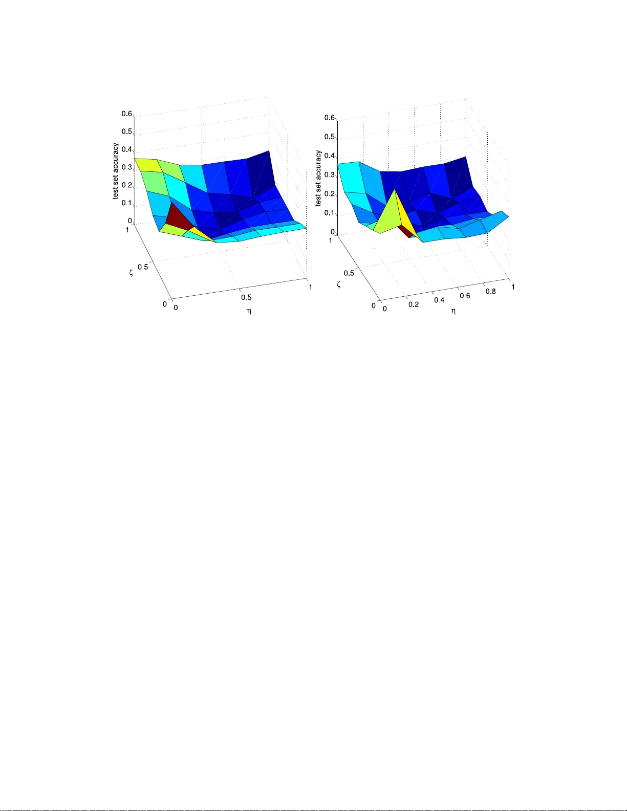
A New Approac h to Colla b orativ e Filtering: Op era tor Estimation with Sp ectral Re gularization Jacob Ab erneth y jake@cs.berkeley.edu Division of Computer Scienc e University of Califo rn ia 387 So da Hal l, Berkeley, CA, USA F rancis R. Bac h francis.bach@mines.or g INRIA - WILLOW Pr oje ct-T e am L ab or atoir e d’Informatique de l’Ec ole Normale Su p ´ erieur e (CNRS/ENS/INRIA U MR 8548 ) 45, rue d’Ulm, 75230 Paris, F r anc e Theo doros Evgeniou theodoros.ev geniou@insead.edu De cision S cienc es and T e chnolo gy Management INSEAD Bd de Constanc e, 77300 F ontaineble au, F r anc e Jean-Philipp e V ert Jean-Philippe.Ver t@Mines-P arisTech.fr Centr e for Computational Biolo gy Mines ParisT e ch, In stitut Curie, In s erm U900 35 rue Saint-Honor´ e, 7730 0 F ontaineble au , F r anc e Abstract W e presen t a general approac h for collabor ativ e filtering (CF) using sp ectral r egularization to lear n linear op erators from “ users” to a s et of p ossibly desir ed “ob jects”. Recen t low- rank type matrix completio n approaches to CF are shown to b e spec ial ca ses. How ever, unlike existing regulariz a tion bas ed CF metho ds, our approach can be used to also incor- po rate information such as attributes of the users or the ob jects—a limita tion of existing regular iz ation bas ed CF metho ds. W e provide nov el re presenter theorems that we use to develop new estimation metho ds. W e then provide learning alg orithms based on low-rank decomp ositions, and test them on a standar d CF da taset. The exp eriments indicate the adv a n tage s of generaliz ing the existing regulariza tion based CF metho ds to incorp orate r e- lated information ab out users and ob jects. Finally , we sho w that certain m ulti-ta s k learning metho ds can b e also seen as s pecial ca ses o f our pr opo s ed appr o ach. 1. In tro duction Collab orativ e fi ltering (CF) refers to th e task of pr edicting pr eferences of a giv en “user” for some “ob jects” (e.g., b o oks, music, pro du cts, p eople, etc.) based on h is/her previously rev ealed pr eferences—t y p ically in the form of purchases or r atings—as well as the rev ealed preferences of other users . In a b ook recommender system, f or example, one w ould like to 1 suggest new b o oks to someone b ased on what she and other users ha ve recen tly purchased or r ated. The ultimate goal of CF is to infer the preferences of users in order to offer them new ob jects. A n umb er o f CF metho ds ha ve b een dev elop ed in the past (Breese et al., 1998, Hec k erman et al. , 2000, Salakh utdin o v et al., 2007). Rece ntly there has b een int erest in CF using regulariza- tion based metho ds (Srebro and Jaakk ola, 2003). This w ork adds to that literature by dev eloping a no ve l general appr oac h to dev eloping regularization based CF metho ds . Recen t regularizatio n based CF metho ds assu me that the only data a v ailable are the re- v ealed preferences, where no other information suc h as bac kground information on the ob jects or u sers is giv en. In this case, one may formulate the problem as that of inf er r ing the con ten ts of a partially observed pr e fer enc e matrix : eac h ro w represent s a user, eac h column represen ts an ob ject (e.g., b ooks or mo vies), and en tries in the matrix represent a giv en u s er’s rating of a giv en ob ject. When the only in formation a v ailable is a set of observ ed u ser/ob ject ratings, the un kno wn en tries in the matrix must b e inferred from the kno wn ones – of which there are t ypically very few relativ e to the size of the matrix. T o mak e usefu l predictions within this setting, regularization b ased CF metho ds make certain assumptions ab out the r elate dness of the ob jects and u sers. The most common assumption is that pr eferences can b e decomp osed into a small n u m b er of f actors, b oth for users and ob jects, r esu lting in the searc h f or a low-rank matrix whic h appro ximates the partially observed matrix of pr eferences (Srebr o and Jaakk ola , 2003). The ran k constrain t can b e inte r p reted as a regularization on the hypothesis space. Since the r ank constr aint giv es rise to a non-con v ex set of m atrices, th e asso ciated optimizat ion problem will b e a difficult non-con vex problem for whic h only h euristic algorithms exist (Srebro and Jaakko la , 2003). An alternativ e f orm ulation, prop osed b y S rebro et al. (2005), s uggests p enalizing the predicted matrix b y its tr ac e norm , i.e., the su m of its singular v alues. An add ed b enefit of th e trace norm regularizatio n is that, with a su fficien tly large regularization parameter, the final solution will b e lo w-rank (F azel et al., 2001, Bac h , 2008). Ho w ever, a k ey limitation of curren t regularization based CF metho ds is that they d o n ot tak e adv anta ge of information, suc h as attributes of users (e.g., gender, age) or ob jects (e.g., b o ok’s author, genre), whic h is often av ailable. Intuitiv ely , such in formation migh t b e usefu l to guide the inference of preferences, in particular for u sers and ob jects with very few kno wn ratings. F or example, at the extreme, users and ob jects with no prior ratings can not b e considered in the standard CF f orm ulation, while their attributes alone could pro vide some basic preference inference. The main contribution of this pap er is to dev elop a general framew ork and sp ecific algo- rithms also based on n o vel represen ter th eorems for the more general CF setting wh ere other information, such as attributes for us er s and /or ob jects, ma y b e a v ailable. More precisely w e s h o w that CF, wh ile t yp ically seen as a p roblem of matrix completion, can b e thought of more generally as estimating a linear op erator from the space of user s to the sp ace of ob j ects. Equiv alently , this can b e view ed as learning a bilinear form b etw een users and ob jects. W e then d ev elop sp e ctr al r e gularization based metho ds to learn suc h linear op erators. When dealing with op erators, rather than matrices, one ma y also w ork with in finite d imension, allo w ing one to consid er arbitrary feature sp ace, p ossibly induced by some k ernel fun ction. Among ke y theoretical con trib utions of this pap er are new repr esen ter theorems, allo w ing 2 us to develo p new general metho ds that learn finitely m any p arameters ev en when working in infi nite dimensional u ser/ob ject feature space. T hese representer theorems generalize the classical repr esen ter theorem for min imizatio n of an emp irical loss p enalized by the norm in a Repro ducing Kern el Hilb ert Space (RKHS ) to more general p enalt y functions and function classes. W e also sho w that, w ith the appropriate c hoice of k ernels for b oth user s and ob jects, w e ma y consider a num b er of existing mac hin e learning metho ds as sp ecial cases of our general framew ork. In p articular, we sho w that several CF metho ds such as r an k constrained optimization, trace-norm regularization, and those based on F rob en iu s norm regularization, can all b e cast as sp ecial cases of sp ectral r egulariza tion on op erator sp aces. Moreo ver, particular c hoices of kernels lead to sp ecific sub-cases suc h as regular matrix completion and m ultitask learning. In the sp ecific ap p licatio n of collab orativ e filtering with the presence of attribu tes, we sh o w th at our generalization of these su b-cases leads to b etter predictiv e p erformance. The outline of th e pap er is as follo ws. In Sectio n 2, w e review the notion of a compact op erator on Hilb ert S pace, and we sho w h o w to cast the collaborative fi ltering pr oblem within this framewo rk . W e then introdu ce sp ectral regularizati on and d iscuss ho w r ank constrain t, trace norm regularization, and F r ob enius norm regularization are all sp ecia l cases of sp ectral regularization. I n S ectio n 3, w e sho w h ow our general f r amew ork encompasses man y existing metho ds by prop er c hoices of the loss fun ction, the kernels, and the sp ectral regularizer. In Section 4, we pro vide three repr esen ter th eorems for op er ator estimation with sp ectral regularization which allo w for efficien t learning algorithms. Finally in Section 5 we present a n umb er of algorithms and describ e sev eral tec h niques to impro ve efficiency . W e test these algorithms in Section 6 on synthetic examples and a widely used mo vie database. 2. Learning compact op erators with sp ectral regularization In this section w e prop ose a mathematical formulat ion for a general CF problem with sp ectral r egularizat ion. W e then sho w in Section 3 how seve r al learnin g problems can b e cast under this general framew ork. 2.1 A general CF formulation W e consider a general CF p roblem in whic h our goal is to mo del the preference of a user describ ed by x for an item d escrib ed b y y . W e denote b y x and y the data ob jects con taining all relev an t or av ailable inf ormation; this could, for example, in clude a unique iden tifier i for the i -th u ser or ob ject. Of course, the users and ob jects ma y additionally b e c haracterized b y attributes, in whic h case x or y would contai n some represen tation of this extra information. Ultimately , we w ould like to consider suc h attribute inform atio n as enco ded in some p ositiv e definite k ernel b et ween users, or equiv alentl y b et w een ob jects. This naturally leads us to mo del the users as elemen ts in a Hilb ert space X , and the ob jects they rate as elemen ts of another Hilb ert space Y . W e assume that our obs erv ation data is in the form of r atings from u sers to ob jects, a real-v alued score representing the user’s preference for the ob ject. Alternativ ely , similar 3 metho ds can b e applied when the observ ations are binary , sp ecifying for in stance wh ether or not a us er considered or selected an ob ject. Giv en a series of N observ ations ( x i , y i , t i ) i =1 ,...,N in X × Y × R , w here t i represent s the r ating of user x i for ob ject y i , the generalized CF pr oblem is then to infer a function f : X × Y → R that can then b e used to predict the r ating of an y user x ∈ X for an y ob ject y ∈ Y b y f ( x , y ). Note th at in our notation, x i and y i represent the user and ob ject corr esp onding to the i -th rating a v ailable. If sev eral ratings of a user for different ob jects are av ailable, as is commonly the case, sev eral x i ’s will b e iden tical in X —a sligh t abu se of notation. W e denote by X N and Y N the linear spans of { x i , i = 1 , . . . , N } and { y i , i = 1 , . . . , N } in X and Y , with resp ectiv e d imensions m X and m Y . F or the function to b e estimated we r estrict ourselv es to b ilinear forms giv en b y: f ( x , y ) = h x , F y i X , (1) for some compact op erator F . W e no w denote by B 0 ( Y , X ) the set of compact op era- tors f rom X to Y . F or an in tro du ction to relev ant concepts in fun ctional analysis, see App endix A. In th e general case we consider b elo w, if X and Y are not Hilb ert s p aces, one could also first map (implicitly) users x and ob jects y into p ossibly in finite dimensional Hilb ert feature spaces Φ X ( x ) and Ψ Y ( y ) and use k ernels. W e refer the reader to App endix A for basic definitions and p rop erties related to compact op erators that are useful b elo w. The in ference problem can no w b e stated as follo ws: Given a tr aining set of r atings, how may we e stimate a “go o d” c omp act op er ator F to pr e dict futur e r atings using (1)? W e estimate the op erator F in (1) from the training data using a standard regularization and statistica l mac h in e learning approac h. In particular, we prop ose to d efine the op erator as the solution of an optimizatio n problem o ve r B 0 ( Y , X ) whose ob jectiv e fu nction balances a data fi tting term R N ( F ), which is small f or op erators that can correctly explain th e training data, with a regularization term Ω( F ). W e no w d escrib e th ese t wo terms in more details. 2.2 Data fitting term Giv en a loss fu nction ℓ ( t ′ , t ) that qu an tifies ho w goo d a prediction t ′ ∈ R is if the tru e v alue is t ∈ R , we consider a fitting term equal to the empirical risk, i.e., the mean loss incur red on the training set: R N ( F ) = 1 N N X i =1 ℓ ( h x i , F y i i X , t i ) . (2) The p articular choic e of the loss function s h ould t ypically dep end on the p recise problem to b e solved and on the nature of th e v ariables t to b e p redicted. See more details in Section 3. In particular, while the representer theorems presente d in Section 4 d o not need an y con v exit y with resp ect to this choic e, the algorithms p resen ted in Section 5 do. 4 2.3 Regularization term F or the regularizatio n term, w e fo cus on a class of sp ectral fu nctions d efined as f ollo ws. Definition 1 A function Ω : B 0 ( Y , X ) 7→ R ∪ { + ∞} is c al le d a sp ectral p enalt y fu n ction if it c an b e written as: Ω( F ) = d X i =1 s i ( σ i ( F )) , (3) wher e for any i ≥ 1 , s i : R + 7→ R + ∪ { + ∞} i s a non-de cr e asing p enalty function satisfying s (0) = 0 , and ( σ i ( F )) i =1 ,...,d ar e the d singular values of F in de cr e asing or der— d p ossibly infinite. Note that by the sp ectral theorem presente d in Ap p endix A, any compact op erator can b e decomp osed into singular v ectors, with singular v alues b eing a sequence that tends to zero. Sp ectral p en alt y functions include as sp ecial cases seve r al functions often encoun tered in matrix completion prob lems: • F or a giv en int eger r , taking s i = 0 for i = 1 , . . . , r and s r +1 ( u ) = + ∞ if u > 0, leads to the fun ction: Ω( F ) = ( 0 if r ank( F ) ≤ r , + ∞ otherwise. (4) In other words, the set of op erators F that satisfy Ω ( F ) < + ∞ is th e set of op erators with rank smaller th an r . • T aking s i ( u ) = u for all i r esults in the trace n orm p en alt y (see App endix A): Ω( F ) = ( k F k 1 if F ∈ B 1 ( Y , X ) , + ∞ otherwise, (5) where we note with B 1 ( Y , X ) the set of op erators with finite trace norm. Such op er- ators are referred to as trace class op erators. • T aking s i ( u ) = u 2 for all i resu lts in the squared Hilb ert-Sc hmidt norm p enalt y (also called squared F rob enius norm for matrices, see App endix A): Ω( F ) = ( k F k 2 2 if F ∈ B 2 ( Y , X ) , + ∞ otherwise, (6) where we n ote with B 2 ( Y , X ) the set of op erators with fi nite squared Hilb ert-Sc hm idt norm. S uc h op erators are referr ed to as Hilb ert Sc h midt op erators. These p articular fu nctions can b e combined together in d ifferen t w a ys. F or example, w e ma y constrain the rank to b e s maller than r wh ile p enalizing the trace norm of the matrix, whic h can b e obtained by setting s i ( u ) = u for i = 1 , . . . , r and s r +1 ( u ) = + ∞ if u > 0. Alternativ ely , if we wan t to p enalize the F rob enius n orm w hile constraining th e rank, w e 5 set s i ( u ) = u 2 for i = 1 , . . . , r and s r +1 ( u ) = + ∞ if u > 0. W e state these tw o choic es of Ω explicitly sin ce we use these in the exp erim ents (see Section 6) or to design efficien t algorithms (see S ectio n 5): T race+Rank Penalt y: Ω( F ) = ( k F k 1 if rank( F ) ≤ r , + ∞ otherwise. (7) F rob enius+ R an k Penal ty: Ω( F ) = ( k F k 2 2 if rank( F ) ≤ r , + ∞ otherwise. (8) 2.4 Op erator inference With b oth a fitting term and a regularization term, we can now formally defin e our inf erence approac h. It consists of finding an op erator ˆ F , if there exists one, that solv es the follo wing optimization problem: ˆ F ∈ arg min F ∈B 0 ( Y , X ) R N ( F ) + λ Ω ( F ) , (9) where λ ∈ R is a p arameter that con trols the trade-off b et ween fitting and r egularization, and where R N ( F ) and Ω( F ) are resp ectiv ely defin ed in (2 ) and (3). W e note that if th e set { F ∈ B 0 ( Y , X ) , Ω( F ) < + ∞} is not empty , then n ecessarily th e solution ˆ F of this optimization problem must s atisfy Ω( ˆ F ) < ∞ . W e sh o w in Sections 4 and 5 how p roblem (9) can b e solv ed in p ractice in particular for Hilb ert spaces of infin ite dimensions. Before exploring such implemen tation-related issues, in the follo wing section we p ro vide sev eral examples of algorithms that can b e deriv ed as particular cases of (9) and highligh t their relationships to existing metho ds. 3. Examples and related approac hes The general form u lation (9) can result in a v ariet y of practical algorithms p otent ially u s eful in different con texts. In particular, three element s can b e tailored to one’s particular needs: the loss fun ction, the ke r nels (or equiv alen tly the Hilb ert spaces), and the sp ectral p en alt y term. W e start this section by some generalities ab out the p ossible c hoices for these elements and their consequences, b efore h ighlighting some particular combinatio n s of choice s relev ant for different applications. 1. The loss function. The c h oice of ℓ defines the empirical r isk thr ough (2 ). It is a classical comp onen t of man y mac hin e learning metho ds , and should t ypically dep end on the type of data to b e predicted (e.g., discrete or contin u ous) and of th e fin al ob jectiv e of the algorithm (e.g., classification, regression or ranking). The c hoice of ℓ also in fluences the algorithm, as discussed in S ectio n 5. As a deep er discussion ab out the loss fu nction is only tangen tial to the current work, w e only consider the square loss here, knowing that other con vex losses may b e considered. 2. The sp ectral p e na lt y function. The c hoice of Ω( F ) defin es the t yp e of constrain t w e imp ose on the op erator that we seek to learn. In Section 2.3, we ga ve several 6 examples of such constraint s including the r ank constraint (4), the trace norm con- strain t (5), the Hilb ert-Schmidt norm constrain t (6), or the trace norm constraint o v er lo w-rank op erators (7). The c h oice of a particular p enalt y might b e guided by some considerations ab out the problem to b e solved, e.g., fi nding lo w-rank op erators as a w ay to d isco ver lo w -d imensional latent structures in the data. On the other h and, fr om an algorithmic p ersp ectiv e, th e c hoice of th e sp ectral p enalty ma y affect the efficiency or feasibilit y of our learning algorithm. C ertain p en alty functions, such as the r ank constrain t for example, will lead to n on -conv ex problems b ecause the corresp onding p enalt y fun ctio n (4) is not con vex itself. Ho wev er, the s ame rank constrain t can v astly reduce the n u m b er of p arameters to b e learned. These algorithmic considerations are discussed in more d etail s in S ectio n 5. 3. The k ernels. Our c hoice of kernels defin es th e inner pro ducts (i.e., embedd ings) of the users an d ob jects in their resp ectiv e Hilb ert sp aces. W e may use a v ariet y of p ossible kernels d ep ending on the problem to b e s olved and on the attributes a v ailable. In terestingly , the c hoice of a particular kernel has n o influ ence on the algorithm, as we sho w later (ho wev er, it d oes of course in fluence the ru nning time of these algorithms). In the cur ren t w ork, w e fo cus on t wo basic k ern els (Dirac k ern els and attribute k ern els) and in Section 3.4 w e d iscuss combining these. • The fi rst k ernel we consider is the Dir ac kernel. When tw o users (resp. t wo ob jects) are compared, the Dirac k ernel return s 1 if they are the same user (resp. ob ject), and 0 otherw ise. In other wo r d s, the Dirac kernel amoun ts to represent in g the u sers (resp. the ob jects) b y orthonormal vec tors in X (resp. in Y ). T his k ern el can b e us ed w hether or not attributes are a v ailable for users and ob jects. W e d enote b y k X D (resp. k Y D ) the Dirac k ernel for the us ers (resp. ob j ects). • The second k ernel w e consider is a k ernel b et ween attributes , when attributes are a v ailable to d escrib e the users and/or ob jects. W e call th is an “attribute k ernel”. This would typically b e a k ernel b etw een v ectors, suc h as the inner pro duct or a Gauss ian RBF ke r nel, when the descriptions of users and /or ob jects tak e the form of v ectors of real-v alued attributes, or any ke r nel on s tructured ob jects (Shaw e-T a ylor and Cristianini, 2004 ). W e denote by k X A (resp. k Y A ) the attributes ke r nel for the us ers (resp. ob jects). In th e follo wing section we illustrate ho w sp ecific com binations of loss, sp ectral p enalt y and ke r nels can b e relev an t for v arious settings. In particular the c hoice of k ern els leads to new metho ds for a r an ge of different estimation pr oblems; namely , matrix completion, m ulti-task learning, and p airwise learning. In Section 3.4 w e consider a new represent ation that allo ws in terp olation b et ween these particular p roblem form ulations. 3.1 Matrix completion When the Dirac ke r n el is used for b oth users and ob jects, then we can organize the data { x i , i = 1 , . . . , n } in to n X groups of iden tical data p oint s and similarly { y i , i = 1 , . . . , n } in to n Y groups. Since we use the Dirac kernel, w e can r epresen t eac h of these groups b y the elemen ts of the canonica l basis ( u 1 , . . . , u n X ) and  v 1 , . . . , v n Y  of R n X and R n Y , 7 resp ectiv ely . A b ilinear form using Dirac kernels only dep en d s on the identiti es of the u sers and the ob jects, and w e only p redict the r ating t i based on the identi ties of the group s in b oth spaces. If we assum e that eac h p air user/ob ject is observe d at most once, the d ata can b e re-arranged in to a n X × n Y incomplete m atrix, the learning ob jectiv e b eing to complete this matrix (indeed, in th is cont ext, it is not p ossible to generalize to nev er seen p oin ts in X and Y ). In this case, our bilinear form fr amework exact ly corresp onds to completing the matrix, since the bilinear fu nction of x and y is exactly equal to u ⊤ i M v j where x = u i (i.e., x is th e i -th p erson) and y = v j (i.e., y is the j -th ob ject). Thus, the ( i, j )-th en try of the matrix M can b e assimilated to the v alue of the bilinear f orm defin ed by the matrix M ov er the pair ( u i , v j ). Moreo v er the sp ectral regularizer corresp onds to the corresp ond ing sp ectral function of the complete matrix M ∈ R n X × n Y . In this con text, find ing a lo w-rank approxima tion of the observ ed en tries in a matrix is an app ealing strategy , w h ic h corresp ond s to taking the rank p en alty constraint (4 ) combined with, for example, the s quare loss error. Th is ho wev er leads to non-conv ex optimization problems w ith m u ltiple lo cal minima, for whic h only lo cal searc h heuristics are kn o wn (Srebro and Jaakko la , 2003). T o circum v ent this issue, conv ex sp ectral p enalt y functions can b e considered. Ind eed, in th e case of b inary preferences, combining the hinge loss func- tion with the trace n orm p enalt y (5) leads to the maximum margin matrix factorization (MMMF) app roac h pr op osed b y Sr ebro et al. (2005), w hic h can b e rewr itten as a semi- definite program. F or the s ake of efficiency , Rennie and Sreb ro (2005) p rop osed to add a constrain t on the rank of the matrix, r esulting in a non-con ve x problem that can never- theless b e handled efficien tly b y classical gradien t descen t tec h n iques; in our setting, this corresp onds to c hanging the trace n orm p en alty (5 ) by the p enalt y (7). 3.2 Multi-task learning It ma y b e the case that w e ha ve attributes only for ob jects y (w e could do the same for attributes for users). In that case, for a fi nite n u m b er of users { x i , i = 1 , . . . , N } organized in n X groups, we aim to estimate a separate fun ction on ob jects f i ( y ) for eac h of the n X users i . Cons id ering the estimation of eac h of th ese f i ’s as a le arning task , one can p ossibly learn all f i ’s simultane ously using a multi-task le arning appr oac h. In order to adapt our general fr amew ork to this scenario, it is natural to consider the attribute kernel k Y A for th e ob jects, w h ose attribu tes are a v ailable, and the Dirac ke r nel k X D for the user s , for whic h no attributes are used. Again the c hoice of the loss fun ction dep ends on the precise task to b e solv ed, and the sp ectral p enalt y function can b e tuned to enforce some sharing of inform ation b et we en differen t tasks. In particular, taking the rank p enalt y fu nction (4) enforces a decomp osition of the tasks (learning eac h f i ) into a limited num b er of f acto r s. Th is r esults in a metho d for multit ask learning based on a lo w-rank representa tion of the p redictor functions f i . Th e resu lting problem, ho w eve r , is not con v ex due to the use of th e non-conv ex rank p enalt y function. A n atural alternativ e is then to replace the rank constrain t b y the trace n orm p enalt y function (5), resulting in a con ve x optimization pr oblem wh en th e loss function is con- 8 v ex. Recen tly , a similar appr oac h wa s indep en den tly pr op osed b y Amit et al. (2007) in the con text of m ulticlass classification and by Ar gyr iou et al. (2008) for multit ask learning. Alternativ ely , another strategy to enforce some constrain ts among the tasks is to constrain the v ariance of th e d ifferen t classifiers. Evgeniou et al. (2005) sho wed that this strategy can b e form u lated in th e framew ork of su pp ort vecto r mac hines b y consid er in g a multitask kernel , i. e., a kernel k multitask o v er the pro duct space X × Y defin ed b et ween an y t wo user/ob ject pairs ( x , y ) and ( x ′ , y ′ ) by: k multitask (( x , y ) , ( x , y )) =  k X D  x , x ′  + c  k Y A  y , y ′  , (10) where c > 0 con trols how the v ariance of the classifiers is constrained compared to the n orm of eac h classifier. As exp lained in App end ix A, estimating a function o v er the pro duct sp ace X × Y by p enalizing th e RKHS norm of the kernel (10) is a particular case of our general framew ork, where we tak e the Hilb ert-Sc hmidt norm (6) as sp ectral p enalt y function, and where the ke r nels b et ween users and b etw een ob jects are resp ectiv ely k X D ( x , x ′ ) + c and k Y A ( y , y ′ ). When c = 0, i.e., when we take a Dirac kernel for the users and an attribute kernel for th e ob jects, then p enalizing the Hilb ert-Sc hmitt norm amoun ts estimating ind ep enden t mo dels f or eac h u s ers, as explained in Evgeniou et al. (2005). Com bin ing t wo Dirac k ernels for users and ob jects, resp ectiv ely , and p enalizing the Hilb ert-Schmitt norm would not b e v ery in teresting, s in ce the s olution wo u ld alw ays b e 0 except on the training p airs. On the other hand , replacing the Hilb ert-Sc hmidt norm defined b y other p enalties suc h as the trace norm p enalt y (5) would b e an in teresting extension when the kernels k X D ( x , x ′ ) + c and k Y A ( y , y ′ ) are used: this w ould constrain b oth the v ariance of the predictor functions f i and their decomp osition into a small n u m b er of factors, which could b e an in teresting approac h in some multit ask learning applications. 3.3 P airwise learning When attributes are a v ailable for b oth u sers and ob jects then it is p ossible to tak e th e attributes k ernels f or b oth of th em. Combining this choice with th e Hilb ert-Schmidt p enalt y (6) results in classical mac hine learning algorithms (e.g., an SVM if the hinge loss is tak en as the loss function) applied to the tensor pr o duct of X and Y . Th is s trateg y is a classical approac h to learn a function o v er pairs of p oints (see, e.g., Jacob and V er t , 2008). Replaci n g the Hilb er t-Schmidt norm b y another sp ectral p enalt y function, su c h as the trace norm, w ould r esult in new algorithms f or learning lo w -rank functions ov er pairs. 3.4 Com bining the attribut e and Dirac k ernels As illustrated in the previous subsections, the setting of the app licat ion often d etermines the com bination of k ern els to b e used for the users and th e ob j ects: typica lly , t wo Dirac k ernels for the standard C F s etting without attributes, one Dirac and one attributes kernel for multi -task problems, and tw o attributes k ernels wh en attributes are a v ailable for b oth users and ob jects and one wish es to learn o v er pairs. There are many situations, ho wev er , w here the attributes a v ailable to describ e the users and/or ob jects are certainly useful for the inference task, bu t on the other h and do not fully 9 c haracterize the users and/or ob jects. F or examp le, if we just kno w the age and gender of users, we wo u ld lik e to use this information to mo del their p references, b ut would also lik e to allo w differen t p references for differen t users even wh en they share the same age and gender. In our setting, this means that w e m a y w ant to us e the attributes kernel in order to utilize known attributes fr om th e users and ob jects du ring infer en ce, b ut also the Dirac k ernel to incorp orate the fact that differen t users and/or ob jects remain d ifferen t ev en w hen they share many or all of their attributes. This n atur ally leads us to consider the follo w ing conv ex combinatio n s of Dirac an d attributes k ernels (Ab erneth y et al. , 2006): ( k X = η k X A + (1 − η ) k X D , k Y = ζ k Y A + (1 − ζ ) k Y D , (11) where 0 ≤ η ≤ 1 and 0 ≤ ζ ≤ 1. These k ern els in terp olate b etw een the Dirac ke r nels ( η = 0 and ζ = 0) and the attributes kernels ( η = 1 and ζ = 1). Com bin ing this c h oice of k ernels with, e.g., the trace norm p enalt y function (5), allo ws us to cont inuously inte r p olate b et wee n different s ettings corresp onding to different “corners” in the ( η , ζ ) square: s tand ard CF with matrix completion in (0 , 0), m ulti-task learnin g in (0 , 1) and (1 , 0), and learning o v er pairs in (1 , 1). The extra degree of fr eedom created when η and ζ are allo w ed to v ary con tin u ously b et ween 0 and 1 provides a prin cipled wa y to optimally balance the influence of the attributes in the function estimation p ro cess. Note that our r epresen tational framew ork encompasses simpler natur al app roac h es to in- clude attribute information for collab orativ e fi ltering: for example, one could consid er com- pleting m atrices using matrices of the form U V ⊤ + U A R ⊤ A + U A S ⊤ A , where U V ⊤ is a lo w-rank matrix to b e optimized, U A and V A are the giv en attributes for the first and second domains, and R A , S A are p arameters to b e learned. This form ulation corresp onds to addin g an un- constrained lo w-rank term U V ⊤ , and the simpler linear predictor from the concatenat ion of attributes U A R ⊤ A + U A S ⊤ A (Jacob and V ert , 2008). O ur approac h imp licitly adds a four th cross-pro duct term U A T V ⊤ A , w here T is estimated f r om data. This exactly corresp onds to imp osing that the lo w rank matrix h as a d ecomp osition whic h in cludes U A and V A as columns. Ou r com bin ation of Dirac and attribute k ernels has the adv antag e of ha ving sp e- cific we ights η and ζ that con trol the trade-off b et ween the constrained and un constrained lo w-rank matrices. 4. Represen t er theorems W e no w present the ke y theoretical results of this p ap er and discu s s ho w the general opti- mization p r oblem (9) can b e solved in pr actic e. A fi rst difficult y with this problem is th at the optimization space { F ∈ B 0 ( Y , X ) : Ω( F ) < ∞} can b e of infi nite d imension. W e note that this can o ccur ev en un der a r ank constrain t, b ecause th e set { F ∈ B 0 ( Y , X ) : rank( F ) ≤ R } is not in cluded in to any finite-dimensional linear subsp ace if X and Y ha ve infinite dimen- sions. In this section, w e sho w that the optimization problem (9) can b e r ep hrased as a finite-dimensional problem, and prop ose practical algorithms to s olv e it in Section 5. Wh ile the reform u latio n of the p roblem as a finite-dimensional prob lem is a simple instance of the r epresen ter theorem when th e Hilb ert-Sc h m idt norm is u s ed as a p enalty function (Sec- 10 tion 4.1), we prov e in Section 4.2 a generalized r epresen ter theorem that is v alid with any sp ectral p enalt y fu nction. 4.1 The case of the Hilb ert-Schmidt p enalty function In the p articular case wh ere the p enalt y function Ω ( F ) is the Hilb ert-Schmidt norm (6), then the set { F ∈ B 0 ( Y , X ) : Ω( F ) < ∞} is the set of Hilb ert-Sc hm idt op erators. As r ecalled in App endix A. this set is a Hilb ert space isometric through (1) to the repro ducing k ernel Hilb ert space H ⊗ of the kernel: k ⊗  x , x ′  ,  y , y ′  =  x , x ′  X  y , y ′  Y , and the isometry translates from F to f as: k f k 2 H ⊗ = k F k 2 = Ω( F ) . As a result, in that case the pr oblem (9) is equ iv alen t to: min f ∈H ⊗  R N ( f ) + λ k f k 2 ⊗  . (12) In that case the represen ter theorem for optimizatio n of emp irical risks p enalized by the RKHS norm (Aronsza jn, 1950, Sc h¨ olk opf et al., 2001) can b e applied to sho w that the solution of (12) necessarily liv es in the linear span of the tr aining d ata. With our notatio n s this translates into the follo wing r esu lt: Theorem 2 If ˆ F is a solution of the pr oblem: min F ∈B 2 ( Y , X ) R N ( F ) + λ ∞ X i =1 σ i ( F ) 2 , (13) then i t is ne c essarily in the line ar sp an of { x i ⊗ y i : i = 1 , . . . , N } , i.e., it c an b e written as: ˆ F = N X i =1 α i x i ⊗ y i , (14) for some α ∈ R N . F or the sak e of completeness, and to highlight why this result is sp ecific to the Hilb ert- Sc hmid t p enalt y fun ction (6), w e rephrase here, with our n otati ons , th e main arguments in the pro of of Sch¨ olk opf et al. (2001). An y op erator F in B 2 ( Y , X ) can b e decomp osed as F = F S + F ⊥ , where F S is the p ro jection of F on to the linear span of { x i ⊗ y i : i = 1 , . . . , N } . F ⊥ b eing orthogonal to eac h x i ⊗ y i in the training set, one easily gets R N ( F ) = R N ( F S ), while k F k 2 = k F S k 2 + k F ⊥ k 2 b y the Pythagorean theorem. As a resu lt a minimizer F of th e ob jectiv e fu nction m us t b e suc h that F ⊥ = 0, i.e., m us t b e in the linear span of the training tensor pr od ucts. 11 4.2 A Represen ter Theorem for General Sp ectral Penalt y F unctions Let us n o w mo v e on to the m ore general situation (9) where a general sp ectral function Ω( F ) is used as regularizati on. Th eorem 2 is usually not v alid in s u c h a case. Its pro of breaks do wn b ecause it is not true that Ω( F ) = Ω ( F S ) + Ω( F ⊥ ) for general Ω, or even that Ω( F ) ≥ Ω( F S ). The follo w ing theorem, whose pro of is presente d in App endix B, can b e seen as a generalized represent er theorem. It sho w s that a solution of (9), if it exists, can b e expand ed ov er a finite basis of d imension m X × m Y (where m X and m Y are the un derlying d imensions of the subspaces where the d ata lie), and that it can b e found as the solution of a fin ite-dimensional optimization problem (with no con ve xity assum ptions on the loss): Theorem 3 F or any sp e ctr al p e nalty function Ω : B 0 ( Y , X ) 7→ R ∪ { + ∞} , let the opti- mization pr oblem: min F ∈B 0 ( Y , X ) , R N ( F ) + λ Ω( F ) . (15) If the set of solutions is not empty, then ther e is a solution F in X N ⊗ Y N , i.e., ther e exists α ∈ R m X × m Y such that: F = m X X i =1 m Y X j =1 α ij u i ⊗ v j , (16) wher e ( u 1 , . . . , u m X ) and  v 1 , . . . , v m Y  form orthonorma l b ases of X N and Y N , r esp e c- tively. Mor e over, in that c ase the c o efficie nts α c an b e found by solving the fol lowing finite- dimensional optimizatio n pr oblem: min α ∈ R m X × m Y R N  diag  X αY ⊤  + λ Ω( α ) , (17) wher e Ω( α ) r efe rs to the sp e ctr al p enalty function applie d to the matrix α se en as an op er ator fr om R m Y to R m X , and X ∈ R N × m X and Y ∈ R N × m X denote any matric es that satisfy K = X X ⊤ and G = Y Y ⊤ for the two N × N Gr am matric e s K and G define d by K ij = h x i , x j i X and G ij = h y i , y j i Y , for 0 ≤ i, j ≤ N . This theorem shows th at, as so on as a sp ectral p enalt y fun ction is used to cont r ol the complexit y of th e compact op erators, a solution can b e searc hed in the finite-dimensional space X N ⊗ Y N , wh ic h in p ractice b oils do w n to an optimizati on problem o ve r the set of matrices of size m X × m Y . Th e d im en sion of th is space migh t how ever b e prohibitiv ely large for real-w orld applications where, e.g., tens of thousand s of users are confron ted to a d atabase of thousands of ob jects. A con ve n ien t w ay to obtain an imp ortant decrease in complexit y (at the exp ense of p ossibly losing conv exity) is b y constraining th e rank of the op erator through an adequate choic e of a sp ectral p enalt y . Indeed, the set of non-zero singular comp onent s of F as an op erator is equal to the s et of non-zero singular v alues of α in (16 ) seen as a matrix. Con s equen tly any constrain t on the rank of F as an op erator results in a constraint on α as a m atrix, from whic h w e d educe: Corollary 4 If, in The or em 3, the sp e c tr al p enalty function Ω is infinite on op er ators of r ank lar ger than R (i.e., σ R +1 ( u ) = + ∞ for u > 0 ), then the matrix α ∈ R m X × m Y in (16) has r ank at most R . 12 As a result, if a rank constraint rank( F ) ≤ r is added to the optimizatio n pr ob lem then the represent er theorem still h olds but the dimension of the parameter α b ecomes r × ( m X + m Y ) instead of m X × m Y , w h ic h is usu ally b eneficial. W e note, ho wev er, th at w h en a r an k constrain t is added to the Hilb ert-Sc hmid t norm p enalt y , then the classical represent er Theorem 2 and the expansion of the solution o v er N vecto rs (14) are not v alid anymore, only Theorem 3 and the expansion (16) can b e used . 5. Algorithms In this section we explain how the optimization problem (17) can b e solv ed in pr actic e. W e first consider a general form ulation, then w e sp ecialize to the situation w here many x ’s and man y y ’s are ident ical; i.e., we are in a matrix completion setting where it may b e adv anta geous to consider other formulations that tak e into account some group structure explicitly . 5.1 Con vex dual of sp ectral regularization When the loss is con ve x, we can d eriv e the con v ex dual problem, whic h can b e h elpful for actually solving the op timization p roblem. Th is could also provi d e an alternativ e p ro of of the representer theorem in that particular s itu ation. F or all i = 1 , . . . , N , we let denote ψ i ( v i ) = ℓ ( v i , t i ) the loss corresp onding to predicting v i for the i -th data p oint. F or simplicit y , w e assume that eac h ψ i is con vex (this is usually met in practice). F ollo wing Bac h et al. (2005), w e let ψ ∗ i ( α i ) denote its F enc hel conjugate defined as ψ ∗ i ( α i ) = max v i ∈ R α i v i − ψ i ( v i ). Minimizers of the optimization problem defin ing the conjugate function are often referred to as F enchel d uals to α i (Bo y d and V anden b er gh e, 2003). I n p articular, w e h a ve the follo wing classical examples: • L e ast-squar es r e gr ession : we hav e ψ i ( v i ) = 1 2 ( t i − v i ) 2 and ψ ∗ i ( α i ) = 1 2 α 2 i + α i t i . • L o gi stic r e gr ession : we h av e ψ i ( v i ) = log(1 + exp( − y i v i )), where y i ∈ {− 1 , 1 } , and ψ ∗ i ( α i ) = (1 + α i t i ) log (1 + α i t i ) − α i t i log( − α i t i ) if α i t i ∈ ( − 1 , 0), + ∞ otherwise. W e also assu me that the sp ectral regularization is suc h that for all i ∈ N , s i = s , where s is a con vex fu nction such that s (0) = 0. In this situation, w e h a v e Ω( A ) = P i ∈ N s ( σ i ( A )). W e can also defi n e a F enchel conjugate for Ω( A ), wh ic h is also a sp ectral fun ction Ω ∗ ( B ) = P i ∈ N s ∗ ( σ i ( B )) (Lewis and Sendov, 2002). Some sp ecial cases of interest for s ( σ ) are: • s ( σ ) = | σ | leads to the trace norm an d then s ∗ ( τ ) = 0 if | τ | is less than 1, and + ∞ otherwise. • s ( σ ) = 1 2 σ 2 leads to the F rob enius/Hilb ert Sc h midt norm and then s ∗ ( τ ) = 1 2 τ 2 . • s ( σ ) = ε log (1+ e σ/ε )+ ε log (1+ e − σ/ε ) is a smo oth appr o ximation of | σ | , whic h b ecomes tigh ter when ε is closer to zero. W e h a v e: s ∗ ( τ ) = 1 ε (1+ τ ) log (1+ τ ) + 1 ε (1 − τ ) log (1 − τ ). Moreo ver, s ′ ( σ ) = τ ⇔ ( s ∗ ) ′ ( τ ) = σ = 1 ε log 1+ τ 1 − τ . 13 Once the representer theorem h as b een applied, our optimization problem can b e rewritten in the primal form in (17): min α ∈ R m x × m y N X i =1 ψ i (( X αY ⊤ ) ii ) + λ Ω( α ) . (18) W e can no w form the Lagrangian, asso ciated with added constraints v = diag( X αY ⊤ ) and corresp onding Lagrange multiplier β ∈ R N : L ( v , α, β ) = N X i =1 ψ i ( v i ) − N X i =1 β i ( v i − ( X αY ⊤ ) ii ) + λ Ω( α ) , and minimize with r esp ect to v and W to obtain the dual pr ob lem, wh ic h is to maximize: − N X i =1 ψ ∗ i ( β i ) − λ Ω ∗  − 1 λ X ⊤ Diag( β ) Y  . (19) Once the optimal dual v ariable β is f ou n d (there are as many of those as there are obser- v ations), then w e can go bac k to α (whic h ma y or ma y n ot b e of smaller size), b y F en chel dualit y , i.e., α is among the F enc hel duals of − 1 λ X ⊤ Diag( β ) Y . Thus, wh en the function s is differen tiable and strictly con vex (whic h implies that the s et of F enchel du als is a singleton), then w e obtain the p rimal v ariables α in closed form from the d u al v ariables β . When s is not different iable, e.g., for the trace n orm th en, follo w ing Amit et al. (2007 ), w e can find the pr imal v ariables by noting that once β is kn o wn, the sin gular v ectors of α are kno wn and we can fin d the singular v alues b y solving a reduced con ve x optimization problem. Computational complexity Note that for optimizatio n , we ha ve t wo strategies: u sing the p rimal problem in Eq. (18) of dimen sion m X m Y 6 n X n Y (the actual dimension of th e underlying data) or usin g the dual problem in Eq. (19) of dimension N (the num b er of ratings). Th e choice b et ween those t w o formulat ions is pr oblem dep end en t. 5.2 Collab orative filtering In the pr esence of (man y) identica l columns and ro w s, w hic h is often the case in collab ora- tiv e filtering situations, the k ern el matrices K and L ha ve some columns (and th u s ro w s) whic h are iden tical, and we can in stead consider the kernel matrices (with their sq u are-root decomp ositions) ˜ K = ˜ X ˜ X ⊤ and ˜ L = ˜ Y ˜ Y ⊤ as the k ern el matrices for all distinct elemen ts of X and Y (let n X and n Y b e their sizes). Then eac h observ ation ( x i , y i , t i ) corresp ond s to a pair of indices ( a ( i ) , b ( i )) in { 1 , . . . , n X } × { 1 , . . . , n Y } , and the primal/dual problems b ecome: min α ∈ R m x × m y n X i =1 ψ i ( δ ⊤ a ( i ) ˜ X α ˜ Y ⊤ δ b ( i ) ) + λ Ω( α ) , (20) where δ u is a v ector with only zero es except at p osition u . Th e d ual function is − N X i =1 ψ ∗ i ( β i ) − λ Ω ∗ − 1 λ ˜ X ⊤ N X i =1 β i δ a ( i ) δ ⊤ b ( i ) ˜ Y ! . 14 Similar to usu al k ern el mac h ines and th e general case presen ted ab o ve, using the p rimal or the du al form ulation for optimization d ep ends on the n u mb er of a v ailable r atings N compared to th e r anks m X and m Y of the kernel matrices ˜ K and ˜ L . Ind eed, th e num b er of v ariables in the primal formulatio n is m X m Y , while in the du al formulation it is N . 5.3 Lo w-ra nk constrained problem W e approxima te the sp ectral norm by an infin itely differentia b le sp ectral fu nction. S ince w e consider in this pap er only infinitely differen tiable loss functions, our p r oblem is th at of minimizing an infin itely differen tiable conv ex fu nction G ( W ) o ver rectangular matrices of size p × q for certain intege r s p and q . As a r esult of our sp ectral regularization, we hop e to obtain (approximate ly) low-rank matrices. In this con text, it has p ro v ed adv anta geous to consider lo w-rank d ecompositions of the f orm W = U V ⊤ where U and V h a v e m < min { p, q } columns (Burer and Monteiro, 2005, Bu rer and Choi, 2006). Burer and Monteiro (2005) ha ve sho wn that if m = min { p, q } then the non-con ve x problem of minimizing G ( U V ⊤ ) with resp ect to U and V ⊤ has no lo cal minima. W e no w pro ve a stronger result in the conte xt of t wice d ifferen tiable functions, n amely that if the global optimum of G has rank r < min { p, q } , then the low-rank constrained p roblem with r ank r + 1 has no lo cal minim um and its global minim um corresp onds to the global minim u m of G . The follo win g theorem m akes this precise (see App en d ix C for p ro of ). Prop osition 5 L et G b e a twic e differ entiable c onvex f u nction on matric es of size p × q with c omp act level sets. L e t m > 1 and ( U, V ) ∈ R p × m × R q × m a lo c al optimum of the function H : R p × m × R q × m 7→ R define d by H ( U, V ) = G ( U V ⊤ ) , i.e., U is such that ∇ H ( U, V ) = 0 and the Hessian of H at ( U, V ) is p ositive semi-definite. If U or V is r ank deficient, then N = U V ⊤ is a glob al minimum of G , i.e., ∇ G ( N ) = 0 . The p revious prop osition sh o ws that if w e ha v e a lo cal minimum for the rank- m problem and if the solution is rank d eficien t, then w e h a ve a solution of the global optimization problem. Th is naturally leads to a sequen ce of reduced p roblems of increasing dimension m , smaller than r + 1, where r is the rank of the global optim um . Ho wev er, the n umb er of iterations of eac h of th e lo cal minimizations and the final rank m cannot b e b ound ed a priori in general. Note th at using a lo w-rank representat ion to solve the trace-norm r egularized p roblem leads to a non-con ve x minimization problem with no lo cal min ima, wh ile simply u sing the lo w - rank repr esen tation without the trace norm p enalt y and p oten tially with a F rob eniu s norm p enalt y , ma y lead to lo cal minima; i.e., we consider instead of Eq. (17) with th e trace norm, the follo wing form ulation: min α ∈ R m X × r , β ∈ R m Y × r R N  diag  X αβ ⊤ Y ⊤  + λ r X q =1 k α (: , k ) k 2 k β (: , k ) k 2 , (21) where α (: , k ) and β (: , k ) are the k -th columns of α and β . In the sim ulation section, we compare the t wo app roac h es on a syn th etic example, and sh o w that the con vex formulation 15 solv ed through a sequence of non-con ve x f orm ulations leads to b etter predictiv e p erfor- mance. 5.4 Kernel learning for sp ectral functions In our collab orativ e filtering con text, th ere are t wo p oten tially useful sources of k ernel learn- ing: learning th e attribute k ernels, or learning the w eight s η and ζ b et ween Dirac k ernels and attribute k ern els. In this section, w e s h o w ho w multiple k ernel learning (MKL) (Lanckriet et al., 2004, Bac h et al., 2004) ma y b e extended to sp ectral regularization. W e first show that the optimization problem that w e ha ve defined in earlier sections only dep ends on the Kroneck er pro du ct of k ernel matrices K ⊗ G : Prop osition 6 The dual solution of the optimization pr oblem in Eq. (22) dep ends only on the matrix K ⊗ G . Pro of It s u ffices to sho w th at for all matrices B , then the p ositive singu lar v alues of X ⊤ B Y only d ep end on K ⊗ G . T he largest singular v alue is defined as the maximum of a ⊤ X ⊤ B Y b o v er unit norm ve ctors a and b . By a change of v ariable, it is equiv alen t to maximize ( X ⊤ ˜ a ) X ⊤ B Y ( Y ⊤ ˜ b ) k X ⊤ ˜ a kk Y ⊤ ˜ b k = v ec ( ˜ b ˜ a ⊤ )( K ⊗ G )vec( B ) v ec ( ˜ b ˜ a ⊤ ) ⊤ ( K ⊗ G )v ec( ˜ b ˜ a ⊤ ) with resp ect to ˜ a and ˜ b (Golub and Loan, 1996). Th u s th e largest p ositiv e singular v alue is ind eed a fu nction of K ⊗ G . Results for other singular v alues ma y b e obtained similarly . This sh o w s that the natural k ernel matrix to b e learned in ou r con text is the Kronec ker pro duct K ⊗ G . W e thus follo w Lanckriet et al. (2004) and consider M ke r nel matrices K 1 , . . . , K M for X and M k ernel matrices G 1 , . . . , G M for Y ; one p ossibilit y could b e to learn a con vex com bin atio n of the matrices K k ⊗ G k b y m inimizing with resp ect to the com bination we ights the optimal v alue of the problem in Eq. (22 ). Ho wev er , unlike the usual Hilb ert norm regularization, this do es not lead to a con vex p roblem in general. W e th us fo cus on the alternativ e form u latio n of the MKL problem (Bac h et al., 2004): we consider th e sum of the predictor fun ctions associated with eac h of th e individual kernel pairs ( K k , G k ) and p enalize by the s um of the norms. That is, if w e let denote X 1 , . . . , X M and Y 1 , . . . , Y M the r esp ectiv e square ro ots of matrices K 1 , . . . , K M and G 1 , . . . , G M , we lo ok for predictor f u nctions w hic h are sums of the M p ossible atomic pred ictor fu nctions, and we p en alize b y the sum of sp ectral fu nctions, to obtain the follo wing optimization p roblem: min ∀ k , α k ∈ R m k x × m k y n X i =1 ψ i M X k =1 ( X k α k Y ⊤ k ) ii ! + λ M X k =1 Ω( α k ) . W e f orm the Lagrangian: L ( v , α 1 , . . . , α M , β ) = n X i =1 ψ i ( v i ) − N X i =1 β i ( v i − M X k =1 ( X α k Y ⊤ ) ii ) + λ M X k =1 Ω( α k ) , 16 and minimize w.r .t. v and α 1 , . . . , α M to obtain the du al pr oblem, w hic h is to maximize − X u ψ ∗ i ( β i ) − X k λ Ω ∗  − 1 λ X ⊤ k Diag( β ) Y k  . (22) In the case of the trace norm, w e obtain supp ort k ernels (Bac h et al., 2004), i.e., only a sparse com bin atio n of matrices end s up b eing u sed. Note that in the d ual formulat ion, there is only one α to optimize, and thus it is preferable to use the d u al formulat ion rather than the primal formulation. This framewo r k can b e natur ally applied to com bine the four corners defin ed in Section 3.4. Indeed, we can form M = 4 ke r nel matrices f or eac h of the four corners and learn a com bination of such matrices. W e sho w in S ectio n 6 ho w the MKL framew ork allo ws to automatica lly combine these four corners without setting the trade-off directly though η and ζ (b y the u s er or through cross-v alidation). 6. Exp erimen t s In this Section w e present sev eral exp erimen tal findings for the algorithms and metho ds discussed ab ov e. Much of th e presen t w ork w as motiv ated b y the problem of collab orativ e filtering and we therefore fo cus s olely within this d omain. As d iscu ssed in Section 3 , b y using op er ator estimation and sp ectral regularization as a framew ork for C F, we ma y utilize p oten tially more information to predict p r eferences. Our pr imary goal n o w is to show that, as one w ould hop e, suc h capabilities do impr o ve prediction accuracy . 6.1 Datasets and Metrics W e present sev eral plots created by exp erimenting on synthetic data. This dataset was generated as f ollo ws: (1) sample i.i.d. multiv ariate f eatures f or x of dimension 6, (2) generate i.i.d. m u ltiv ariate features for y of dimension 6 as well , (3) sample z from a random bilinear form in x and y plus some noise, (4) restrict the obser ved feature sp ace to only 3 features for b oth x and y . S ince part of the data is discarded , the lab el cannot b e p erfectly predicted b y the kno wn features. On the other hand, since we k eep some of them, kno wing and us in g these attributes should w ork b etter than not u s ing them. In other w ords , we exp ect that setting η and ζ to b e v alues other than 0 or 1 should provide b etter p er f ormance. W e also exp erimen ted w ith the well- kn o wn Mo vieLens 100k dataset from the Gr ou p Lens Researc h Group at the Univ ersit y of Minnesota. Th is dataset consists of ratings of 1682 mo vies by 943 us er s . Eac h user p ro vided a rating, in the f orm of a score from { 1 , 2 , 3 , 4 , 5 } , for a small su bset of th e movie s. Eac h user rated at least 20 movies, and the total n umb er of ratings a v ailable is exactly 100,00 0, av eraging ab out 105 p er user. This d atase t w as rather appropriate as it included attribute information for b oth the mo vies and the users. Eac h mo vie w as lab eled with at least one among 19 genres (e.g., action or adv ent u re), while the users’ attributes in cluded age, gender, and an o ccupation among a list of 21 o ccupations (e.g., administrator or artist). W e con v erted the u sers’ age attribute to a set of bin ary features that d escrib es to wh ich of 5 age categorie s the user b elongs. 17 Figure 1: Comparison b etw een t w o s p ectral p enalties: the trace norm (left) and the F r ob e- nius norm (right), eac h with an additional fixed r ank constrain t as describ ed in Section 5.3. Eac h surf ace plot displays p erformance v alues o v er a range of η and ζ v alues, all obtained u sing the synthetic dataset. The minimal v alue ac hieved by the trace norm is 0.1222 and the one ac hieved by the rank constrain t is 0.1540. All test set accuracies are measured as th e r oot mean squared error av eraged o ve r 10-fold cross v alidations. In particular, we fo cus on the comparisons of in termediate v alues of η and ζ , compared to the four “corners” of th e η /ζ − parameter sp ace: • η = 0 , ζ = 0: matrix completion • η = 0 , ζ = 1 and η = 1 , ζ = 0: multi-task learning on user s or ob jects • η = 1 , ζ = 1: pairwise learning 6.2 Results T racenorm V ersus Low-rank In Figure 1, we pr esen t t w o p erform an ce plots o ver the η /ζ parameter space, b oth obtained u s ing the synthetic dataset. Th e left plot disp la y s the results when utilizing th e trace norm sp ectral p enalt y . Here we used the lo w rank decomp osition formulation describ ed in Section 5.3 which (by Prop osition 5 ) has no lo cal minima. The plot on the right utilizes th e s ame rank-constrained formulatio n , but with a F rob enius norm p en alt y instead. T h e trace norm constrained algorithm p erform s sligh tly b etter. Moreo ver, b est p redictiv e p erformance is ac h ieved in b oth cases in the middle of the square and not at an y of the four corners. Kernel Learning In Figure 2, w e sh ow the test set accuracy as a function of the reg- ularization parameter, when w e u se the k ern els corresp onding to the four corners as the 18 Figure 2: Learning the k ernel: test set accuracy vs. regularization parameter. Minimum v alue is 0.14. four b asis k ernels. W e can see that w e reco ve r similar p er f ormance (error of 0.14 instead of 0.12) than by searc hin g ov er all η and ζ ’s. T h e same algorithm could also b e us ed to learn k ernels on the attributes. P erformance on Mo vieLens Data Figure 3 sho ws the predictiv e accuracy in RMSE on the Mo vieLens dataset, obtained by 10-fold cross-v alidation. T h e heat plot pro vides some insigh t on the relativ e v alue, for b oth mo vies and users, of the giv en attribute k ern els versus the s im p le identit y k ernels. Th e corners hav e higher v alues th an some of the v alues inside the s q u are, showing that the b est balance b et ween attribute and Dirac k ernels is ac hiev ed for η , ζ ∈ (0 , 1). 7. Conclusions W e ha ve presente d a metho d for solving a generalized matrix completion p roblem where we ha ve attributes describ in g the matrix dimensions. The pr oblem is formalized as the problem of inferring a linear compact op erator b et wee n t wo general Hilb ert spaces, wh ich generalizes the classica l finite-dimensional matrix completio n problem. W e in tro duced the notion of sp ectral regularizatio n for op erators, which generalized v arious sp ectral p enalizations for matrices, and pr o v ed a general represen ter theorem for this setting. V arious approac hes, suc h as standard lo w rank matrix completion, are sp ecial cases of our metho d. It is partic- ularly relev ant f or CF applications where attribu tes are a v ailable for users and /or ob j ects, and preliminary exp erim ents confi rm the b enefits of our metho d. An interesti n g direction of futu r e researc h is to explore further the m ulti-task learning algorithm we obtained with lo w-rank constrain t, and to s tudy the p ossibility to deriv e on-line imp lemen tations that ma y b etter fit the need for large-scale app licat ions wh ere training data are cont inuously increasing. On the theoretical side, a b etter understand ing of the effects of norm and rank regularizations and their in teraction w ould b e of considerable in terest. 19 Figure 3: A heat plot of p erformance for a range of kernel parameter c hoices, η and ζ , usin g the Mo vieLens dataset. App endix A. Compact operator s on Hilb ert spaces In this app endix, w e recall basic definitions and pr op erties of Hilb ert space op erators. W e refer the in terested reader to general b o oks (Brezis, 1980, Berlinet and Thomas-Agnan, 2003) for more details. Let X and Y b e t wo Hilb ert s paces, with resp ectiv e in n er pro du cts d enoted b y h x , x ′ i X and h y , y ′ i Y for x , x ′ ∈ X and y , y ′ ∈ Y . W e denote by B ( Y , X ) the set of b ounded op erators from X to Y , i.e., of contin u ous linear mappings from Y to X . F or any t wo elements ( x , y ) in X × Y , w e denote by x ⊗ y their tensor pr o duct , i.e., the linear op er ator from Y to X defined by: ∀ h ∈ Y , ( x ⊗ y ) h = h y , h i Y x . (23) W e denote by B 0 ( Y , X ) the set of c omp act linear op erators from Y to X , i.e., the set of linear op erators that map the unit b all of Y to a relativ ely compact set of X . Alternativ ely , they can also b e defin ed as th e limit of finite r an k op erators. When X and Y h a v e fi nite d imensions, then B 0 ( Y , X ) is simp ly the set of linear mappings from Y to X , w hic h can b e represented b y the set of matrices of dimens ions dim ( X ) × dim ( Y ). In that case the tensor pro duct x ⊗ y is represented by the matrix xy ⊤ , where y ⊤ denotes the transp ose of y . F or general Hilb ert sp aces X and Y , an y compact linear op erator F ∈ B 0 ( Y , X ) adm its a sp e ctr al de c omp osition : F = ∞ X i =1 σ i u i ⊗ v i . (24) 20 Here the the sing u lar values ( σ i ) i ∈ N form a sequence of n on -n egat ive real num b ers such that lim i →∞ σ i = 0, and ( u i ) i ∈ N and ( v i ) i ∈ N form orthonormal families in X and Y , r esp ec- tiv ely . Although the v ectors ( u i ) i ∈ N and ( v i ) i ∈ N in (24) are not u n iquely defined for a giv en op erator F , th e set of singular v alues is u niquely defined. By con ve ntion w e den ote by σ 1 ( F ) , σ 2 ( F ) , . . . , the successiv e sin gular v alues of F ranked by decreasing ord er. The r ank of F is the num b er rank( F ) ∈ N ∪ { + ∞} of str ictly p ositiv e sin gular v alues. W e no w describ e three sub classes of compact op erators of particular relev ance in the rest of this pap er. • The set of op erators with fi nite rank is denoted B F ( Y , X ). • The op erators F ∈ B 0 ( Y , X ) that satisfy: ∞ X i =1 σ i ( F ) 2 < ∞ are called H ilb ert-Schmidt op erators. They form a Hilb ert s p ace, denoted B 2 ( Y , X ) , with inner p r od uct h· , ·i X ⊗Y b et wee n basic tensor pro ducts giv en by:  x ⊗ y , x ′ ⊗ y ′  X ⊗Y =  x , x ′  X  y , y ′  Y . (25) In particular, the Hilb ert-Schmidt norm of an op erator in B 2 ( Y , X ) is giv en b y: k F k 2 = ∞ X i =1 σ i ( F ) 2 ! 1 2 . Another useful c haracterization of Hilbert-Schmidt op erators is the follo wing. Eac h linear op erator F : Y → X u n iquely defin es a bilinear function f H : X × Y → R b y f ( x , y ) = h x , F y i X . The set of functions f F asso ciate d to the Hilb ert-Schmidt op erators forms itself a Hilb ert space of functions X × Y → R , wh ic h is the repro du cing k ern el Hilb ert sp ace of the pro du ct kernel defi ned for (( x , y ) , ( x ′ , y ′ )) ∈ ( X × Y ) 2 b y k ⊗  ( x , y ) ,  x ′ , y ′  =  x , x ′  X  y , y ′  Y . • The op erators F ∈ B 0 ( Y , X ) that satisfy: ∞ X i =1 σ i ( F ) < ∞ are called tr ac e-class oper ators. The set of trace-cla ss op erators is denoted B 1 ( Y , X ) . The tr ac e norm of an op erator F ∈ B 1 ( Y , X ) is giv en b y: k F k 1 = ∞ X i =1 σ i ( F ) . Ob vious ly th e follo w ing orderin g exists among these v arious classes of op erators: B F ( Y , X ) ⊂ B 1 ( Y , X ) ⊂ B 2 ( Y , X ) ⊂ B 0 ( Y , X ) ⊂ B ( Y , X ) , and all inclusions are equalities if X and Y h av e finite dimens ions. 21 App endix B. Pro of of Theorem 3 W e s tart with a general result ab out the decrease of singular v alues for compact op erators comp osed with pro jection: Lemma 7 L et G and H b e two Hilb ert sp ac es, H a c omp act line ar subsp ac e of H , and Π H denote the ortho g onal pr oje ction onto H . Then for any c omp act op er ator F : G 7→ H it holds that: ∀ i ≥ 1 , σ i (Π H F ) ≤ σ i ( F ) . Pro of W e use the classical charact erization of th e i -th singular v alue: σ i ( F ) = max V ∈V i ( G ) min x ∈ V , k x k G =1 k F x k H , where V i ( G ) denotes the set of all linear subspaces of G of dimens ion i . No w, obser v in g that for an y x w e h a v e k Π H F x k H ≤ k F x k H pro ves the Lemma. Giv en a training set of patterns ( x i , y i ) i =1 ,...,N ∈ X × Y , rememb er that w e denote b y X N and Y N the linear subs p aces of X and Y spanned by the training p atterns { x i , i = 1 , . . . , N } and { y i , i = 1 , . . . , N } , resp ectiv ely . F or any op erator F ∈ B 0 ( Y , X ), let us now consid er the op erator G = Π X N F Π Y N . By constru ction, F and G agree on the training patterns, in the sense that for i = 1 , . . . , N : h x i , G y i i X = h x i , Π X N F Π Y N y i i X = h Π X N x i , F Π Y N y i i X = h x i , F y i i X . Therefore F and G hav e the same empirical r isk: R N ( F ) = R N ( G ) . (26) No w, b y d enoting F ∗ the adjoin t op erator, w e can use Lemma 7 and the fact that the singular v alues of an op erator and its adj oint are the same to obtain, f or any i ≥ 1: σ i ( G ) = σ i (Π X N F Π Y N ) ≤ σ i ( F Π Y N ) = σ i (Π Y N F ∗ ) ≤ σ i ( F ∗ ) = σ i ( F ) . This implies that the sp ectral p enalt y term satisfies Ω( G ) ≤ Ω( F ). Combined w ith (26), this sho ws that if F is a solution to (15), then G = Π X N F Π Y N is also a s olution. Observing that G ∈ X N ⊗ Y N concludes the pro of of the first part of Theorem 3, r esu lting in (16). W e ha ve n o w redu ced the optimizatio n problem in B 0 ( Y , X ) to a fi nite-dimensional opti- mization o ver the matrix α of size m X × m Y . Let us now rephr ase the optimization problem in this finite-dimensional s pace. Let us first consider the sp ectral p enalt y term Ω( F ). Given the decomp osition (16), the non-zero singular v alues of F as an op erator are exactly the non-zero sin gular v alues of α as a matrix, as so on as ( u 1 , . . . , u m X ) and  v 1 , . . . , v m Y  form orthonorma l bases of X N and 22 Y N , resp ectiv ely . In ord er to b e able to express the empirical r isk R N ( F ) w e m u s t ho wev er consider a decomp osition of F o ver the training patterns, as: F = N X i =1 N X j =1 γ ij x i ⊗ y j . (27) In order to expr ess the singular v alues from this exp r ession let us introduce the Gr am matric es K and G of the training patterns, i.e., the N × N matrices defined for i, j = 1 , . . . , N b y: K ij = h x i , x j i X , G ij = h y i , y j i Y . W e note th at b y d efi nition the ranks of K and G are resp ectiv ely m X and m Y . Let us no w factorize these t w o matrices as K = X X ⊤ and G = Y Y ⊤ , where X ∈ R N × m X and Y ∈ R N × m Y are any squ are ro ots, e.g., obtained by k ernel PC A or Cholesky decomposi- tion (Fine and Sc heinb erg, 2001 , Bac h and Jordan, 2005). The matrices X and Y pro vide a repr esen tation of th e pattern in t wo orthonormal bases which w e denote b y ( u 1 , . . . , u m X ) and  v 1 , . . . , v m Y  . I n particular w e ha v e, for any i, j ∈ 1 , . . . , N : x i ⊗ y j = m X X l =1 m Y X m =1 X il Y j m u l ⊗ v m , from which we d educe: F = m X X l =1 m Y X m =1   N X i =1 N X j =1 X il Y j m γ ij   u l ⊗ v m . Comparing this expression to (16 ) w e d educe th at: α = X ⊤ γ Y . The empirical error R N ( F ) is a fu n ction of f ( x l , y l ) for l = 1 , . . . , N . F rom (27), w e see that: f ( x l , y l ) = N X i =1 N X j =1 γ ij K il G lj , and therefore the vect or of p redictions F N = ( f ( x l , y l )) l =1 ,...,N ∈ R N can b e rewritten as: F N = diag( K γ G ) = d iag  X αY ⊤  . W e can n o w replace th e empirical r isk R N ( F N ) by R N  diag  X αY ⊤  and the p enalt y Ω( F ) by Ω( α ) to deduce the optimization pr ob lem (17) from (15), which concludes the pro of of Theorem 3. App endix C. P ro of of Prop osition 5 Since the function has compact leve l sets, we m a y assume that we are r estricted to an op en b ounded subset of R p × q where the second and first deriv ativ es are uniformly b ounded. W e 23 let denote C > 0 a common upp er b ound of all deriv ativ es. Th e gradient of the fu nction H is equal to ∇ H =  ∇ G ⊤ U ∇ G V  , while the Hessian of H is the follo wing quadratic form: ∇ 2 H [( dU, dV ) , ( dU, dV )] = 2 tr dV ⊤ ∇ GdU + ∇ 2 G [ U dV ⊤ + dU V ⊤ , U dV ⊤ + dU V ⊤ ] . Without loss of generalit y , we may assume that the last columns of U and V are equal to zero (this can b e done b y rotation of U or V ). The zero gradien t assump tion implies that ∇ G ⊤ U = 0 and ∇ GV = 0. While if w e tak e dU and dV with the first m − 1 columns equal to zero, and last columns equal to arbitrary u and v , then the second term in the Hessian is equ al to zero. T he p ositivit y of the first term implies that for all u and v , v ⊤ ∇ Gu > 0, i.e., the gradient of G at N = U V ⊤ is equ al to zero, and th us we get a stationary p oin t and th us a global minim u m of G . References J. Ab ernethy , F. Bac h , T. Evgeniou, and J.-P . V ert. Low-rank matrix factorizat ion with attributes. T ec hnical Rep ort N24/06 /MM, E cole des Mines de Paris, 2006 . Y. Am it, M. Fink, N. Srebr o, and S. Ullman. Unco vering shared structures in m u lticla ss classification. In Pr o c e e dings of the 24th international c onfer enc e on M achine le arning , pages 17–24, New Y ork, NY, USA, 2007. ACM. A. Argyriou, T. Evgeniou, and M. P ontil . Con v ex m u lti-task f eature learning. Machine L e arning , 2008. T o app ear. N. Aronsza jn. Th eory of repro ducing k ern els. T r ans. Am. Math. So c. , 68:337 – 404, 1950. F. R. Bac h. Consistency of trace n orm m inimizatio n . J. Mach. L e arn. R es. , 9:1019–10 48, 2008. F. R. Bac h and M. I. Jordan. Predictiv e lo w-rank decomp osition for ke r nel metho ds. In ICML ’05: Pr o c e e dings of the 22nd international c onfer enc e on Machine le arning , pages 33–40 , New Y ork, NY, USA, 2005 . ACM. F. R. Bac h, G. R. G. Lanckriet, and M. I. Jordan. Multiple kernel learning, conic dualit y , and the SMO algorithm. In ICML ’04: P r o c e e dings of the twenty-first international c onfer e nc e on Machine le arning , page 6, New Y ork, NY, USA, 2004. A CM. F. R. Bac h, R. Thibaux, and M. I. Jordan. Compu ting regularizatio n paths for learning m ultiple k ernels. In La wrence K . Saul, Y air W eiss, and L ´ eon Bottou, editors, A dvanc es in Neur al Information Pr o c essing Systems 17 , pages 73–80, Cam br idge, MA, 2005. MIT Press. A. Berlinet and C . Thomas-Agnan. R epr o ducing Kernel Hilb ert Sp ac es in Pr ob ability and Statistics . Kluw er Academic Publishers, 2003. S. Bo yd and L. V andenb erghe. Convex Optimization . Cambridge Univ. Press, 2003. J. S. Breese, D. Hec k erman, and C. Kadie. Em pirical analysis of p redictiv e algorithms for collaborative fi ltering. In 14th Confer enc e on Unc ertainty in Artificial Intel ligenc e , pages 43–52 , Madison, W.I., 1998. Morgan Kaufman. 24 H. Brezis. Ana lyse F onctionnel le . Masson, 1980. S. A. Bu rer and C. Choi. Compu tational enhancemen ts in lo w-r ank semidefin ite program- ming. Optimization Metho ds and Softwar e , 21:493– 512, 2006 . S. A. Bur er and R. D. C . Mon teiro. Lo cal min ima and con ve r gence in lo w-r an k semidefin ite programming. M athematic al Pr o gr amming , 103:427– 444, 2005. T. E v geniou, C. Micc h elli, and M. Pon til. Learning m u ltiple tasks with k ern el metho ds. J. Mach. L e arn. R es. , 6:615–63 7, 2005 . M. F azel, H. Hindi, and S. Bo yd. A rank minimization h euristic with applicatio n to min imum order s ystem approxima tion. In Pr o c e e dings of the 200 1 Americ an Contr ol Confer enc e , v olume 6, pages 4734–4 739, 2001 . S. Fine and K. Sc heinb erg. E fficien t SVM tr ainin g using lo w -rank k ernel representati ons . J. Mach. L e arn. R es. , 2:243–26 4, 2001. G. H. Golub and C. F. V an Loan. Matrix Computations . John s Hopkins Universit y Press, 1996. D. Hec ke r man, D. M. C hic k ering, C. Mee k, R . Roun thw aite, and C. Kadie. Dep endency net wo r ks for inf erence, collab orativ e filtering, and data visualizatio n . J. Mach. L e arn. R es. , 1:49–75, 2000. L. Jacob and J.-P . V ert. Efficien t p eptide-MHC-I binding prediction for alleles with f ew kno wn binders. Bioinformatics , 24(3):358–3 66, F eb 2008. G. R. G. Lanckriet, N. Cr istianini, L. El Ghaoui, P . Bartlett, and M. I. Jordan. Learning the k ernel matrix with semidefinite p r ogramming. Journal of Machine L e arning R ese ar ch , 5: 27–72 , 2004. A. S. Lewis and H. S. S endo v. Twice different iable sp ectral fu nctions. SIAM J. Mat. Anal. App. , 23(2):36 8–386, 2002 . J. D. M. Ren nie and N. Srebro. F ast maximum m argin matrix factorizatio n for collab orativ e prediction. In Pr o c e e dings of the 22nd international c onfer e nc e on M achine le arning , pages 713–71 9, New Y ork, NY, USA, 2005. A CM P ress. R. Salakh u tdino v, A. Mnih, and G. Hin ton. Restricted b oltzmann mac hines for collab orativ e filtering. I n ICML ’07: Pr o c e e dings of the 24th international c onfer enc e on Machine le arning , pages 791–79 8, New Y ork, NY, USA, 2007. A CM. B. Sch¨ olk opf, R. Herbrich, and A. J. Smola. A generalized r epresen ter theorem. In Pr o c e e d- ings of the 14th Annual Confer enc e on Computatio nal L e arning The ory , vo lum e 2011 of L e ctur e N otes i n Computer Scienc e , pages 416–426, Berlin / Heidelb erg, 2001. Spr inger. J. Sh a we-T a ylor and N. C ristianini. Kernel Metho ds for Pattern Analysis . Cam b ridge Univ ersity Press, 2004. 25 N. Sreb r o and T. Jaakk ola. W eigh ted low-rank appro ximations. In T. F a wcet t and N. Mishra, editors, Pr o c e e dings of the Twentieth International Confer enc e on M achine L e arning , p ages 720–727. AAAI Press, 2003. N. Sr ebro, J . D. M. Rennie, and T. S. J aakk ola. Maxim u m-margin matrix factoriz ation. In L. K. Saul, Y. W eiss, and L. Bottou, editors, A dv. Neur al. Inform. Pr o c ess Syst. 17 , pages 1329–1 336, Cam brid ge, MA, 2005. MIT Press. 26