SiZer for Censored Density and Hazard Estimation

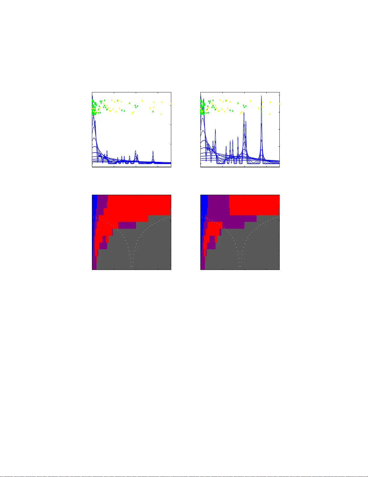
SiZer for Censored Densit y and Hazard Est imation ∗ Jianc heng Jiang Departmen t of Mathematics and Statistics Univ ersit y of North Carolina Charlotte, NC 28223, USA J. S. M arron Departmen t of Statistics Univ ersit y of North Carolina Chap el Hill, NC 27599, USA June 06, 2008 Abstract The SiZe r metho d is e x tended to nonpara metric hazar d estimation and also to censored density and ha zard e stimation. The new method allows quick, visual s ta - tistical inference ab o ut the impo rtant issue of statistica lly s ignificant increa ses and decreases in the smo o th cur ve estimate. This e x tension has re q uired the o p ening of a new av en ue of research on the interface betw een statistical inference and scale space. KEY W ORDS: Scale space, Smoothing, Visual inference. 1 In tro duction Nonparametric hazard rate estimation is a standard to ol in surviv al analysis, d ating bac k at least to W atson and Leadb etter (1964a,b) and Rice and Rosen blatt (1976). F or practical use, a critica l issu e is u nderstand in g wh ere the hazard rate curve increase s and where it decreases. A confounding issue is the bandwidth, i.e. the windo w width or smo othing parameter. SiZer addresses b oth of these problems, in the con text of ∗ J. S. Marron was supported by NSF Gran t DMS-9971649. 1 nonparametric d ensit y and regression estimation, by com bining a scale space approac h to smo othing with a u seful visualization of sim ultaneous statistical inferen ce. The extension of SiZer dev e lop ed in this pap er is not straigh tforw ard. Th e ob vious idea of simp ly plugging reweig h ted data into SiZer give s in v a lid statistic al inference. Hence, a careful statistical accoun ting for the rewe igh ting is devel op ed. Some examples are sho wn in Section 2. Mathematical dev elopmen t is giv en in Section 3. Computational issu es are discussed in Section 4. It is s traigh tforw ard to simulta neously d ev elop these id eas f or (i) hazard estimation; (ii) ce nsored densit y estimat ion; (iii) ce nsored hazard estimation. This is b ecause all three of these cases fit very simply into a general form of estimator, us ing an elegan t common notation, p erh aps fir s t pu blished by Patil (1990, 1993). Hence all three cases are treated sim ultaneously here. F or reasons of present ation, v arious asp ects o f this pap er are usually illustrated b y fo cusing on just one of the th ree cases first. Some other imp ortan t relat ed references include T anner and W ong (198 3), Marron and Padge tt (1987 ), Lo, Mac k and W ang (198 9), Sarda and Vieu (1991), M ¨ uller and W ang (1994 ), Gonz´ alez-Ma nt eiga, Ma rron, and Cao (1996 ), K ousassi and Singh (1997), Stute (1999), Hess, Serachito p ol and Bro wn (1999 ), and Jiang and Doksum (200 3). Man y readers p erhaps understand that when d ata are ce nsored, it is imp ortan t to prop erly adjust for the bias that th is creates, using Kaplan-Meier weigh ts. An example, whic h shows that this bias can seriously impact SiZer inf erence, can b e found in Section 1.1 of Jiang and Marron (2003). K aplan-Meier we igh ts, and there app lication in curve estimation, can b e thought of in sev eral w a ys. An insightful view is to consid er the data in time order. All un censored observ atio ns, that app ear b efore an y censored observ ations, receiv e equal w eigh t. After the first censored obs erv ation app ears, later u ncensored ob- serv a tions receiv e more weigh t, etc. The intuitiv e conten t of the resulting Kaplan Meier w eigh ts is that the later un censored observ a tions, can b e thought of as representing b oth themselv es and also a f raction of the earlier ce nsored o bserv ations in the data set. An example, which illustrates ho w letting one d ata p oin t represent seve ral can seriously im- 2 pact S iZer inference, is give n in Section 1.2 of J iang and Marron (200 3), in th e somewhat differen t con text of d ata rounding. See Fi gure 5 of Chaudh uri and Marron (1999) for another illustratio n of the data roundin g ph enomenon. If re-w e igh ted data are simp ly plugged in to SiZer, then treating the later un censored observ ations as seve ral data p oints, will affe ct the SiZer map in the same w a y , creating in v alid inference. This p roblem is addressed by revising the SiZer inf erence, through a careful v ariance calculation, wh ic h results in corr ect inference. 2 Examples Figure 1 sh o ws a censored SiZer analysis of the S tanford Heart T ransp lant Data , from Kalbfleisc h and Prentice (198 0). The data consisting of 103 observ ations, originally f rom Cro wley and Hu (197 7) are the sur viv a l times (in da ys) of p oten tial heart transplan t recipien ts fr om their date of acceptance into the transplant p r ogram. T h ere is censoring since some patient s w ere lost to follo w u p b efore they died and s in ce some patien ts were still alive on the closing d ate of the study . Analysis from th e p oin t of view of densit y estimation is sho wn in Figures 1a and 1c. This sho ws that th ere are man y deaths v ery so on after tr an s plan tation, and a long decreasing tail. Because of the r elativ ely p o or wa y in whic h the kernel densit y estimato r handles b oun daries, see e.g. Figure 2.16 of W and and Jones (1995) , at larger scales th e estimates fir s t increase at the left edge. SiZer shows th at b oth the o v erall d ecrease (the large red r egion) is statistically significant, and s o are the b oun dary effects (the thin blue region righ t at the edge). F or these data there is more in terest in analysis of the h azard rate, as done in Figures 1b and 1d. The hazard rate is carefully d efined in Section 3, but the intuitiv e idea is the instant aneous rate at wh ich patients die. The estimate is a reweig ht ing of the k ernel densit y estimate, as can b e seen from the fac t that the small scale spikes in Figure 1b are simply magnifications of those in Figure 1a, bu t the sca le is more appr opriate for 3 surviv al consider ations. A central question is: when is the hazard rate increasing, and when is it decreasing? The co lor sc heme o f SiZer is w ell suited to address this issue. F ur thermore, this qu estion is muc h more directly answered by th e SiZ er approac h, than b y more conv e nt ional confidence in terv als. The red in the m iddle left of the SiZer map in Figure 1d shows that the hazard r ate signifi cantly d ecreases d u ring that time p erio d, i.e. as transplan ts “settle in”, c hances of sur viv al in crease. The red near the top on the righ t sho ws that there is also a longer term improv ement of the c hances of su rviv al after one has survive d for a substanti al p erio d. These findin gs are consisten t with those of Jiang and Doksum (2003). An inconsis- tency is the b lue r egion at t he left end. As n oted ab o v e this is d u e to p o or b ound ary b ehavio r of the kernel d ensit y estimator th at un derlies th is infer en ce. The lo cal p olyno- mial estimator d evelo p ed by Jiang and Doksum (2003) a v oids this problem, w hic h is why their h azard estimate is mostly monotonically decreasing. An interesting op en problem is to adapt SiZ er ideas to the Jiang and Doksum lo cal p olynomial hazard estimator. Figure 2 sho ws a S iZ er analysis of the device lifetime data of Aarset(19 87). These data are uncensored and consist of 102 observ atio ns. The d ensit y estimates in Figure 2a su ggest a “U-shap e” density . Ho w ev er the SiZer map in Figure 2c flags only the right hand p eak as statistically significan t. This is lik ely due to the same inefficiency of the ke rnel den sit y estimator near the b oun dary . Of more in terest for these data is th e hazard rate analysis sho wn in Figures 2b a nd 2d. The dominan t color in the SiZ er map is blue whic h sho ws that the h azard rate generally increases o v er time, wh ic h is consistent with the expected w earing o v er time of mec hanical comp onent s. A disapp oin ting feature of the family of hazard estimates in Figure 2b, is that there is a spike only on the righ t sid e, wh ile other analyses, including Aarset(1987) and Mudholk ar, Sriv a sta v a and Kollia (1996) find a “batht ub” sh ap e, that in cludes a spik e on the left as well . This again is b ecause of the p o or b oun dary b eha vior of th e k ernel d ensit y estimator. This problem could also b e addressed by a v ersion of hazard estimation S iZ er th at is based on the lo cal p olynomial metho d of Jiang and Doksum 4 500 1000 1500 0 2 4 6 x 10 −3 Figure 1a Figure 1c log10(h) 0 500 1000 1500 1 1.5 2 2.5 3 500 1000 1500 0 2 4 6 8 x 10 −3 Figure 1b Figure 1d log10(h) 0 500 1000 1500 1 1.5 2 2.5 3 Figure 1: Da ys to death afte r heart transplant. Jitter plot, and family of censored densit y estimates in Figure 1a, w ith corresp onding SiZer map in Figure 1c. F amily of censored hazard estimates in Figure 1 b, w ith corr esp onding S iZer map in Figure 1d . (2003 ). Both of these examples illustrate an imp ortan t p rop erty of SiZer: it provides a gener- ally goo d big picture assessment for initial explorat ory purp oses. Ho w ev er, for addressing an y sp ecific problem, e.g. the b oundary questions b rought up in Figures 1 and 2, it may not b e as effectiv e as a m etho d that sp ecifically targets that issue (although w e do not kno w of a curr en tly implemented metho d that giv es b etter statistical inference of this t yp e at the b oun dary). Hence we prop ose SiZer as a b r oad based metho d for in itially fin ding structure in data (and for the perh aps more important task o f quic k ly und er s tanding what 5 20 40 60 80 0 0.05 0.1 Figure 2a Figure 2c log10(h) 0 20 40 60 80 0 0.5 1 1.5 2 20 40 60 80 0 1 2 Figure 2b Figure 2d log10(h) 0 20 40 60 80 0 0.5 1 1.5 2 Figure 2: Device lifetime data. F amily of censored densit y estimates in Figure 2a, w ith corresp ondin g SiZ er m ap in Figur e 2c . F amily of censored hazard estimates in Figure 2b, with corresp ond in g SiZer map in Figure 2d. structures are mere sample artifacts). After one has an idea ab out what to lo ok for, then other metho ds can pro vide deep er insight s. Of ten the n ext usefu l step is mo delling, e.g. as done b y Mu dholk a r, Sriv asta v a and K ollia (1996) for the device lifetime data. 3 Mathematical Dev elo pmen t Our extension of S iZer is most transparen tly explained in the con text of hazard rate estimation. Hence this is d ev elop ed in Section 3.1. Then the e xtension to censored 6 densit y and censored hazard estimation is done in S ection 3.2. 3.1 Hazard Rat e Mathematics F or d ata X 1 , ..., X n indep en d en t, ident ically distribu ted with cumulativ e distribution func- tion F ( x ), and probab ility d ensit y f ( x ) = F ′ ( x ), the maxim um likelihoo d estimate of F is the empirical cum ulativ e d istribution fu nction F n ( x ) . The k ernel d ensit y estimate of f is b f h ( x ) = n − 1 n X i =1 K h ( x − X i ) , where K h ( · ) = 1 h K  · h  , for the k ernel function K and the bandwidth h . F or f supp orted on (0 , ∞ ) the hazard rate is λ ( x ) = f ( x ) / [1 − F ( x ) ] , and its cumulat iv e is Λ ( x ) = R x 0 λ ( u ) du. W atson and Leadb etter (1964a) sh o w ed, but see for example Pr op osition 1 of Shorac k and W ellner (1986) for a muc h differen t wa y to arrive at the same conclusion, that a natural estimate of th e hazard rate is b λ h ( x ) = n − 1 n X i =1 K h ( x − X i ) 1 − F n ( X i ) (1) = n X i =1 K h  x − X ( i )  n − i , where the X ( i ) are the ord er statistics, with X (1) ≤ · · · ≤ X ( n ) . Deriv ativ es are estimated b y differen tiation. Th e densit y deriv ative , f ′ ( x ), is esti- mated b y b f ′ h ( x ) = n − 1 n X i =1 K ′ h ( x − X i ) , (2) and the h azard rate deriv a tiv e, λ ′ ( x ), is estimated by b λ ′ h ( x ) = n − 1 n X i =1 K ′ h ( x − X i ) 1 − F n ( X i ) = n X i =1 K ′ h  x − X ( i )  n − i , where K ′ h ( x ) = ∂ ∂ x K h ( x ) = 1 h 2 K ′  x h  . The v ariance of the density deriv ativ e estimate is: v ar  b f ′ h ( x )  = v ar n − 1 n X i =1 K ′ h ( x − X i ) ! = n − 1 v ar  K ′ h ( x − X i )  . 7 Denote b y s 2 ( y 1 , . . . , y n ) = n − 1 P n i =1 y 2 i − ( n − 1 P n i =1 y i ) 2 and K ′ 0 ,i = K ′ h ( x − X i ) . Then the v a riance factor ab o v e is estimated by the sample v a riance s 2  K ′ 0 , 1 , ..., K ′ 0 ,n  = n − 1 n X i =1  K ′ 0 ,i  2 − n − 1 n X i =1 K ′ 0 ,i ! 2 (3) = n − 1 n X i =1  K ′ 0 ,i  2 −  b f ′ h ( x )  2 . (4) Using the appr o ximation F n ( x ) ≈ F ( x ) , the v ariance of the d eriv ative hazard rate is appro ximated by v ar  b λ ′ h ( x )  ≈ var n − 1 n X i =1 K ′ h ( x − X i ) 1 − F ( X i ) ! = n − 1 v ar  K ′ h ( x − X i ) 1 − F ( X i )  . Except for the fact that F is u nkno wn the v ariance factor here could b e estimated by the sample v a riance s 2  K ′ F , 1 , ..., K ′ F ,n  , where for an y cum ulativ e distrib ution function H ( x ), d ep endence on x and h is suppressed in th e notation K ′ H,i = K ′ h ( x − X i ) 1 − H ( X i ) . (5) Applying F n ( x ) ≈ F ( x ), we get th e app r o ximation s 2  K ′ F n , 1 , ..., K ′ F n ,n  . (6) This is an imp ortant p oin t w here th ere is a critical differen ce b et w een this deve lopmen t, and simply us in g the rewe igh ted data in o rdinary SiZer. In particular, the v ariance facto r (6), no w app ropriately uses the weig hts. Th us, an isola ted p oin t with a h ea vy w eigh t is no longer flagged as significant, b ecause the v ariance estimate also increases when the w eigh ts are hea vier. SiZer gets its “simulta neous infer en ce” prop erties (i.e. it addresses the multiple com- parison problem) using a “num b er of indep end ent blo c ks” calculation d one in Section 3 8 of Chaudhuri and Marron (1999). The b asis of this is the Effectiv e S ample S ize: E S S h ( x ) = P n i =1 K h ( x − X i ) K h (0) , (7) whic h measures the “num b er of p oints in eac h k ernel windo w” (this is exactly true if K is the uniform density win do w). C orrect adaptation to the hazard con text requir es yet another careful t wist. Naiv e reweig ht ing would suggest that d en ominators of 1 − F ( X i ) should b e inserted. But th e indep end ent blo c ks calculatio n is based on the num b er of indep endent pieces of in formation, so instead th e formula (7) should b e retained in the same form. Th us a hazard rate v ersion of S iZer comes from mo difying the density estimation v ersion, replaci ng the terms K ′ h ( x − X i ) in (2) b y K ′ h ( x − X i ) / [1 − F n ( X i )] , and replacing the v a riables K ′ 0 ,i in (3 ) b y K ′ F n ,i . 3.2 Censored Est imation Mathematics Censored data comes in the f orm ( X 1 , δ 1 ) , ..., ( X n , δ n ), where X i = min ( T i , C i ) and δ i = 1 ( T i ≤ C i ), where 1( A ) is t he indicato r of ev en t A w hic h equals 1 if A happ ens and 0 otherwise. Assume that T 1 , ..., T n are indep enden t, id en tically distributed with cumulativ e dis- tribution fu nction F ( x ) and that C 1 , ..., C n are indep enden t (and indep endent of the T i ), iden tically distributed with cum ulativ e distribution fu n ction G ( x ). Note that the cumu- lativ e distrib ution function of X i , is L ( x ), where the corresp onding cum ulativ e su rviv al function is L ( x ) = F ( x ) G ( x ), using the notation H ( x ) = 1 − H ( x ), f or any cumulativ e distribution function H ( x ) . The goal is estimation of the surviv al probabilit y densit y f ( x ) = F ′ ( x ) and the corresp ondin g hazard rate λ ( x ). The cum ulativ e distribu tion functions F and G can be estimated by the Kaplan Meier 9 (1958 ), i.e. Pro d uct Limit, estimators giv en by F n and G n resp ectiv ely , where F n =        1 − Q X ( i ) ≤ x  n − i n − i +1  δ ( i ) , if x ≤ X ( n ) 0 , if x > X ( n ) , and G n is d efined similarly to F n but with δ ( i ) replaced b y 1 − δ ( i ) , and the  X ( i ) , δ ( i )  are the ord er statistics v ersion of th e data with X (1) ≤ · · · ≤ X ( n ) . A natural k ernel densit y estimate of f is b f h ( x ) = n − 1 n X i =1 δ i K h ( x − X i ) G n ( X i ) . F or f supp orted on (0 , ∞ ) the corresp onding estimate of the hazard r ate is b λ h ( x ) = n − 1 n X i =1 δ i K h ( x − X i ) G n ( X i ) F n ( X i ) = n X i =1 δ ( i ) K h  x − X ( i )  n − i . Note that these hav e a stru cture v ery similar to the hazard r ate estimator (1), which is wh y it is str aigh t forwa rd to extend SiZer to these cases as w ell. Deriv ativ es are again estimated by different iation. The d ensit y deriv ativ e, f ′ ( x ), is estimated by b f ′ h ( x ) = n − 1 n X i =1 δ i K ′ h ( x − X i ) G n ( X i ) . The hazard r ate d eriv ative , λ ′ ( x ), is estimated by b λ ′ h ( x ) = n − 1 n X i =1 δ i K ′ h ( x − X i ) L n ( X i ) . The v ariance of the density deriv ativ e estimate is: v ar  b f ′ h ( x )  = v ar n − 1 n X i =1 δ i K ′ h ( x − X i ) G n ( X i ) ! = n − 1 v ar  δ i K ′ h ( x − X i ) G n ( X i )  , and for th e hazard rate v ar  b λ ′ h ( x )  = v ar n − 1 n X i =1 δ i K ′ h ( x − X i ) L n ( X i ) ! = n − 1 v ar  δ i K ′ h ( x − X i ) L n ( X i )  . 10 Using the approximati on metho ds leading to (6), these v ariance factors are estimated by s 2  δ 1 K ′ G n , 1 , ..., δ n K ′ G n ,n  , (8) using again the n otation (5), and by s 2  δ 1 K ′ L n , 1 , ..., δ n K ′ L n ,n  (9) resp ectiv ely . The E ffective S ample S ize follo ws in a similar spirit. Again the basis is the n um b er of indep enden t pieces of uncensored data, resulting in the form ula E S S h ( x ) = P n i =1 δ i K h ( x − X i ) K h (0) . Th us the censored densit y and censored hazard rate version of SiZer come fr om mo difying the densit y estimation ve rsion, replacing th e term s K ′ h ( x − X i ) in (2) by δ i K ′ h ( x − X i ) / G n ( X i ) and δ i K ′ h ( x − X i ) / L n ( X i ) resp ectiv ely , and b y replacing the v ari- ables K ′ 0 ,i in (3 ) b y K ′ G n ,i and K ′ L n ,i resp ectiv ely . 4 F ast Computation Because SiZer r elies on a large num b er of smo oths, it is imp ortan t to u se a fast compu- tational metho d. Sev eral such are discussed by F an and Ma rron (1994). The binn ed approac h is esp ecially wel l suited to SiZer. Details of the b inned imp lemen tation of b f ′ h ( x ) are similar to those given in Chaudhuri and Marron (1999), whic h are b ased on those of F an and Marron (1994) , except that the k ernels are n o w divided by appropriate cumulativ e d istr ibution fun ctions. I n particular, for the equally spaced grid of p oints { x j : j = 1 , ..., g } , let the corresp ond ing bin coun ts (computed b y some metho d , w e h a v e alw a ys used th e “linear binnin g” describ ed in F an and Marron (1994)) b e { c 0 ,j : j = 1 , ..., g } . Then for density SiZ er b f ′ h ( x j ) ≈ n − 1 S ′ 0 ( x j ) , 11 where S ′ 0 ( x j ) = P g j ′ =1 κ ′ j − j ′ c 0 ,j ′ and κ ′ j − j ′ = K ′ h ( x j − x j ′ ) . The app ro ximated standard deviation of b f ′ h ( x j ), is b sd ( x j ) = n − 1 / 2 v u u u t n − 1 g X j ′ =1  κ ′ j − j ′  2 c 0 ,j ′ −   n − 1 g X j ′ =1 κ ′ j − j ′ c 0 ,j ′   2 . The censored and hazard v ersions of SiZer requir e rec onsideration of the linear binn ing algorithm. When a data p oint X i is betw ee n grid p oints x j and x j +1 , linear binn in g assigns w eigh t w i,j = X i − x j x j +1 − x j to th e bin cente red at x j , and w eigh t w i,j +1 = x j +1 − X i x j +1 − x j to th e bin cente red at x j +1 , and w eigh t 0 to all other bin s. These result in bin counts c 0 ,j = n X i =1 w i,j . F or a generic estima ted cum ulativ e distribu tion fu n ction H n , these bin counts are r eplaced b y c H n ,j = n X i =1 w i,j δ i H n ( X i ) . This results in the b inned app ro ximation to the generic estimator: n − 1 n X i =1 δ i K ′ h ( x − X i ) H n ( X i ) ≈ n − 1 S ′ H n ( x j ) , where S ′ H n ( x j ) = g X j ′ =1 κ ′ j − j ′ c H n ,j ′ , T o s im ilarly ap p ro ximate b sd , use b sd ( x j ) = n − 1 / 2 v u u u t n − 1 g X j ′ =1  κ ′ j − j ′  2 c H n ,j ′  c H n ,j ′ e c 0 ,j ′  −   n − 1 g X j ′ =1 κ ′ j − j ′ c H n ,j ′   2 , 12 where the factor o f  c H n ,j ′ c 0 ,j ′  in the second moment term giv es the s econd factor of 1 H n that app ears in the second moment . Finally , the binn ed ve rsion of the Effectiv e Sample Size needs to b e based on the u nadjuste d bin count s of the uncensored data E S S = P g j ′ =1 κ j − j ′ e c 0 ,j ′ K h (0) , where e c 0 ,j = P n i =1 w i,j δ i and κ j − j ′ = K h ( x j − x j ′ ) . 5 Computational details The results in this p ap er we re obtained using Matlab. Th e co des are a v ailable from S tev e Marron at h ttp://www.stat.unc.edu/p ostscript/pap ers/marron/soft w are/ 6 Discuss W e extend the SiZer to censored densit y and hazard rate estimation. T his extension requires a s tatistical accoun ting f or the reweigh ti ng. Our censored densit y estimation metho d is obvio usly applicable to un-censored cases. Th e SiZ er of densit y and hazard rate estimate allo ws one to make quic k, v isu al statistical inferences on the issue of statistical ly significan t increases and decreases in the smo oth densit y and hazard rate estimate. References [1] Aarset, M. V. (1987) Ho w to iden tify a bath tub hazard rate, IEEE T r ansactions on R eliability , R-36, 106-108. [2] Chaud huri, P . and Marr on, J. S. (1999) S iZer for exploration of structure in curves, Journal of the Americ an Statistic al A sso ciation , 94, 807-823. [3] Crowle y , J. an d Hu, M. (1977). Co v ariance Analysis of Heart T ransplant Surv iv al data, J ournal of the Americ an Statistic al A sso ciation , 72, 27 – 36. 13 [4] Gonz´ alez-Ma n teiga, W., Marr on, J. S. and Cao, R. (1996) Bo otstrap selectio n of the sm o othing parameter in nonparametric hazard rate estimatio n, Journal of the Americ an Statistic al Asso ciatio n , 91, 1130-1140. [5] Hess, K. R., S erac hitop ol, D. M. and Bro wn, B. W. (1999) Hazard f u nction estima- tors: a sim ulation study , Statistics in Me dicine , 18, 3075-308 8. [6] Jiang, J. and Marron, J. S. (2003 ) S iZer for Censored Densit y and Haza rd E stimation. Man uscript. See the w ebsite ht tp://www.stat.unc.edu/p ostscript/pap ers/marron [7] Jiang, J. and Doksum, K. (2003) On Lo cal P olynomial Estimation of Hazard F un c- tions and Their Deriv ativ es und er Ran d om Censoring, In “ Mathematic al Statistics and Applic a tions: F estschrift f or Constanc e van Ee den ”, Eds. M. Mo ore, S. F r o da and C. L’eg er. I MS Lecture Not es and Monograph Ser ies 42, 4 63-482 . Ins titute of Mathematica l Statistics, Bethesda, MD. [8] Kalbfleisc h, J. D. and Prentice , R. I. (1980 ) The sta tistic a l analys is of failur e time data , Wiley , New Y ork. [9] Kaplan, E. L. and Meier, P . (1958 ) Nonparametric estimation from incomplete ob- serv a tions, Journal of the Americ an Statistic a l Asso ciation , 53, 457-481. [10] Kousassi, D. A. and Singh, J. (199 7) A s emip arametric ap p roac h to hazard esti- mation with randomly censored observ atio ns, Journal of the Americ an Statistic al Asso ciation , 92, 1351-135 6. [11] Lo, S. H., Mac k, Y. P . and W ang, J. L. (1989 ) Density and h azard rate esti mation for censored data v ia strong representati on of the Kaplan-Meier estimator, Pr ob ability The ory and R elate d Fields , 74, 461-47 3. [12] Marron, J. S. and P adgett, W. J. (1987) Asymptotically optimal b andwidth selec- tion f or k ernel densit y estimators from randomly righ t censored samples, Annals of Statistics , 15, 1520- 1535. 14 [13] Mudholk ar, G. S., Sr iv asta v a, D. K. and Kollia, G. D. (1996 ) A generalizat ion of the W eibull distribu tion with application to the analysis of su rviv al data, Journal of the Americ an Statistic al Asso ciatio n , 91, 1575-1583. [14] M ¨ uller, H. G. and W ang, J. L. (1 994) Ha zard rate estimati on under random censorin g with v aryin g kernels and band widths, B iometrics , 50, 61-76 . [15] P atil, P . N. (1990) Automatic smo othing parameter selection in hazard rate estima- tion, PhD Dissertation, Univ ersit y of North Carolina, Institute of S tatistics, Mimeo Series # 2033. [16] P atil, P . N. (1993) On the least squares cross-v alidation band w idth in h azard rate estimation, Anna ls of Statistics , 21, 1792-1810 . [17] Rice, J. and Rosen blatt, M. (19 76) Es timation of th e log survivor function and hazard function, Sankhya, A , 38, 60-7 8. [18] Sarda, P . and Vieu, P . (1991) Smo othing p arameter selection in hazard rate estima- tion, Statistics and Pr ob ability L etters , 11, 429-434. [19] Stute, W. (1999) Nonlinear censored regression, Statistic a Sinic a , 9, 1089-1102 . [20] Shorac k, G. R. a nd W ellner, J. A. (1986) Empiric al pr o c esses with applic ations , Wiley , New Y ork. [21] T anner, M. A. and W ong, W. H. (1 983) The estimation of the hazard function from randomly censored data by the kernel metho d , Annals of Statistics , 11, 989-993. [22] W atson, G. S . and Leadb etter, M. R. (1964 a) Hazard Analysis, I, Biometrika , 5 1, 175-1 84. [23] W atson, G. S. an d Leadb etter, M. R. (196 4b) Hazard Analysis, I I, Sankhya A , 26, 110-1 16. 15