Objective Bayesian analysis under sequential experimentation

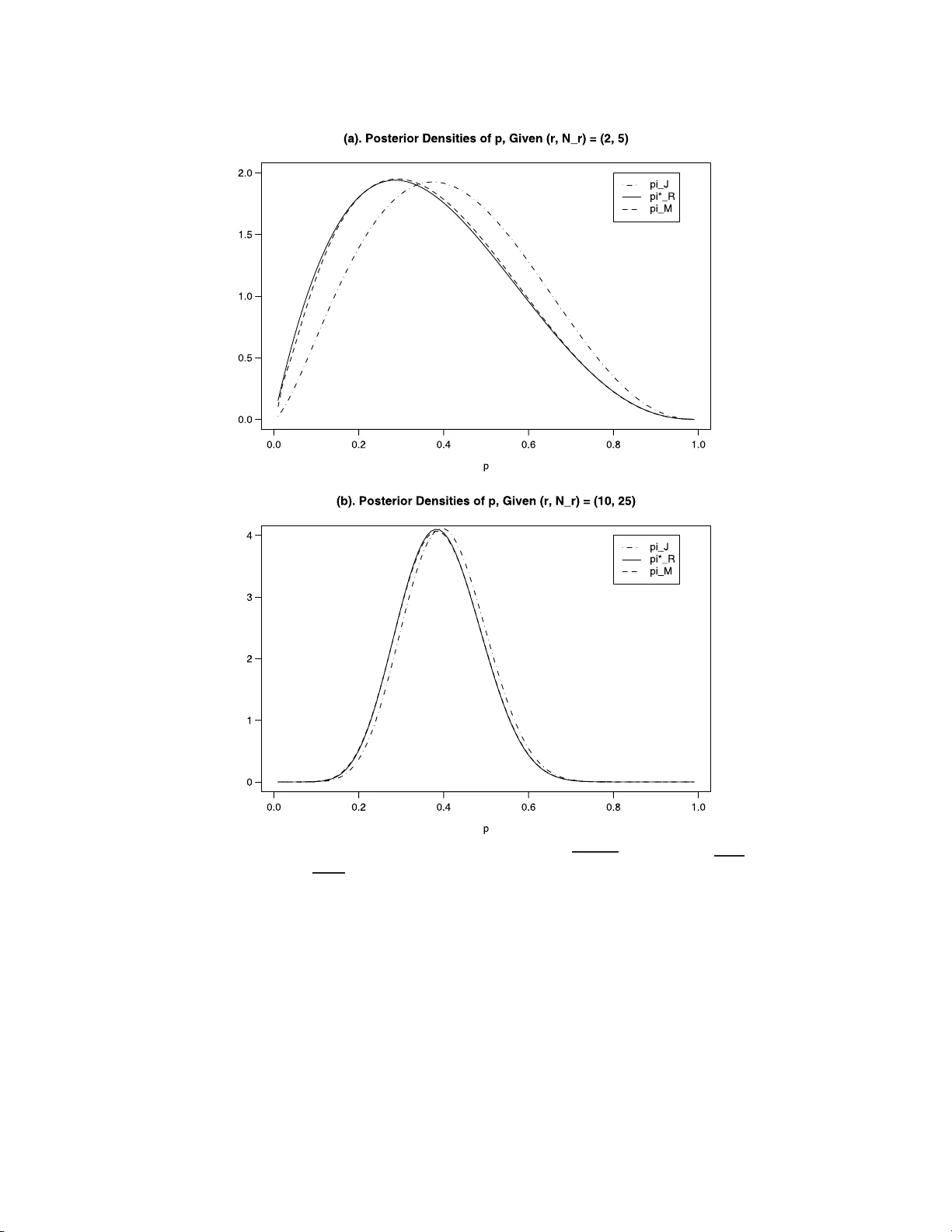
IMS Collectio ns Pushing the Limits of Con temp orary Statist ics: Contributions in Honor of Jay an ta K. Ghosh V ol. 3 ( 2008) 19–32 c  Institute of Mathe matical Statistics , 2008 DOI: 10.1214/ 07492170 80000000 20 Ob jectiv e Ba y esian analysis under sequen tial exp erimen tation ∗ Dongc h u Sun 1 and James O. Berger 2 University of Missouri-Columbia and Duke University Abstract: Ob j ectiv e priors for sequen tial exp eriments are considered. Com- mon priors, suc h as the Jeffreys pri or and the r eference pri or, wil l t ypically depend on the stopping rule used for the sequen tial experi men t. New expres- sions for reference p riors are obtaine d in v ari ous con te xts, and computational issues in v olving suc h prior s are c onsidered. Con ten ts 1 Int ro duction . . . . . . . . . . . . . . . . . . . . . . . . . . . . . . . . . . . 19 2 Noninformative prior s with a known sto pping r ule . . . . . . . . . . . . . 20 2.1 Notatio n and the Jeffreys-r ule prio r . . . . . . . . . . . . . . . . . . . 20 2.2 Reference pr iors . . . . . . . . . . . . . . . . . . . . . . . . . . . . . . 22 3 A tw o -parameter exp onential family . . . . . . . . . . . . . . . . . . . . . 23 3.1 The mo del a nd reference prior s . . . . . . . . . . . . . . . . . . . . . 23 3.2 Pr obability matching pr iors for a sequential ex per iment . . . . . . . 24 4 Computation . . . . . . . . . . . . . . . . . . . . . . . . . . . . . . . . . . 26 4.1 Br ute force computation . . . . . . . . . . . . . . . . . . . . . . . . . 2 6 4.2 The tw o-dimensional case . . . . . . . . . . . . . . . . . . . . . . . . 2 7 4.3 Mo dified reference priors . . . . . . . . . . . . . . . . . . . . . . . . . 27 Ac knowledgmen ts. . . . . . . . . . . . . . . . . . . . . . . . . . . . . . . . . . 30 References . . . . . . . . . . . . . . . . . . . . . . . . . . . . . . . . . . . . . . 30 1. In troductio n Bay esian analysis using o b jective or default priors has r eceived considerable a tten- tion; cf. Datta and Mukerjee [ 17 ], Bernar do [ 6 , 7 ] Berger and Ber nardo [ 4 ], Berger [ 3 ], Ghosh, Delampady a nd Sama nt a [ 21 ], and references therein. The la tter b o o k, in particular, contains an excellent discussion of the is s ues and controv ersies in volv- ing ob jective prio r s, reflecting the many years of leaders hip of J . K. Ghosh in the field (along with his many coa uthors). See, for example, [ 13 , 20 , 22 , 23 ]. ∗ Supported by the NSF Gran ts DM S-01-03265, SES-03-51523 and SES-07-20229, and the NIH Gran t R01-MH071418. 1 Departmen t of Statistics, Universit y of Missouri -Columbia, 146 Middlebush Hall, Columbia, MO 65211-6100, USA, e-mail: sund@mis souri.ed u ; url: www.stat .missour i.edu/ dsun 2 Departmen t of Statistical Science, Duk e Unive rsity , Box 90251, Durham, NC 27708-025 1, USA, e-mail : berger@s tat.duke .edu ; url : www.stat. duke.edu / be rger AMS 2000 subje c t classific ations: Pr imary 62L12, 62C10; secondary 62F15, 62L10. Keywor ds and phr ases: exp ected stopping time, frequen tist cov erage, Jeffreys’ pr ior, p osterior distributions, refer ence pri or, sequen tial exp erimenta tion. 19 20 D. Sun and J. O. Ber ger A common ob jective prior is the Jeffre y s pr ior [ 27 ], which is prop or tional to the square ro ot of the determinant of the Fishe r info r mation matr ix. T he Jeffreys pr ior is quite us e ful for a single par ameter mo del, but can b e seriously deficient for m ulti- parameter models ; this ha s led to prefer ence for r eference pr io rs in multiparameter situations (cf. Be rger and Bernar do [ 5 ] and Bernardo [ 7 ]). Almost all results on o b jective priors hav e been for fixed sample size exp e riments. In practice, how ever, statistical exper iment s a re often conducted se q uent ially , with a known stopping rule (cf. Siegmund [ 30 ] and Ghosh, Sen and Mukhopadhy ay [ 24 ]). Bartholomew [ 2 ] a nd Geisser [ 19 ] intro duced the notio n that ob jective priors for a sequential exp eriment should de p end on the ex pe c ted stopping time. Y e [ 3 8 ] derived the refere nce prior for sequential exper iment s when the exp ected stopping time depends on the parameter of interest only . In this pap er w e ge ne r alize Y e’s result in v arious dir ections, and provide so me new computationa l to ols for use with priors that dep end on exp ected stopping times. The pap er is ar ranged as follows. Section 2 reviews the Fisher information matrix fo r sequential exp eriments with a known stopping rule, derives the Jef- freys/refer ence prior fo r illustrative one-para meter examples, and then pr ovides an expression for multiparameter reference prio rs when the stopping r ule satisfies a certain pr o p erty . In Section 3, refere nc e pr iors and ma tch ing priors (cf. Datta and Mukerjee [ 17 ]) are der ived for Bar- Lev a nd Reiser’s [ 1 ] tw o-parameter exp onential family . Illustrations are given for nor mal distributions with se veral commonly used stopping times. Computation of ex p ected stopping times is often difficult, so that utilization of reference priors for s e quential ex per iments is t ypically challenging. In Section 4, an approximation to the refere nc e prio r for sequential exp er iment s is intro duced which is exa ct under some circumstances, seems to b e a reasona ble approximation in genera l, and allows for muc h simpler computation. 2. Noninformative priors with a known stopping rule 2.1. Notation and the Jeffr eys-ru le pri or W e assume that X 1 , X 2 , . . . , is an i.i.d. sequence o f random v a riables with den- sity f ( x | θ ) that is r e gular (W alker [ 35 ]). Here θ is a q × 1 vector of unknown parameters . Let N denote a pro pe r stopping time for the sequen tial exp er iment – s e e Govindara julu [ 25 ] for a definition, which als o is a s ource for the following well-kno wn lemma : Lemma 2.1. L et I ( θ ) b e the Fisher information matrix b ase d on X 1 . U nder the pr op er stopping time N , the Fisher information b ase d on ( X 1 , . . . , X N ) is I ∗ = E θ ( N ) I ( θ ) . (2.1) The Jeffreys-rule pr ior [ 27 ] fo r θ is defined as the s q uare ro o t of the deter- minant of the Fisher infor mation ma trix. In the fixed sample size case, this is π J ( θ ) ∝ | I ( θ ) | 1 / 2 . F or the sequential exp eriment, it fo llows from the ab ov e lemma that Jeffreys’ prio r is π ∗ J ( θ ) ∝ { E θ ( N ) } q/ 2 | I ( θ ) | 1 / 2 ∝ { E θ ( N ) } q/ 2 π J ( θ ) . (2.2) Example 2.1. Let N r be a r andom v ar iable with a negative binomial distribution N B ( r, p ), wher e r is a p os itive integer and p ∈ (0 , 1). L e t X 1 , X 2 , . . . b e a s equence Obje ctive se quential exp erimentation 21 of Ber noulli r andom v ariables with success pr obability p . N r can b e viewed as a stopping time for this Bernoulli sequence as follows: N r = inf { n ≥ 1 : X 1 + · · · + X n = r } . The proba bility of N r is P ( N r = k ) =  k − 1 r − 1  p r (1 − p ) k − r , for k = r, r + 1 , . . . . An easy computation yields E p ( N r ) = r /p . Since the Jeffreys rule prio r for a Bernoulli random v ariable is π J ( p ) ∝ 1 / p p (1 − p ), it follows from ( 2.2 ) that the Jeffreys rule prio r for the negative binomial distr ibution is π ∗ J ( p ) ∝ r p π J ( p ) ∝ 1 p √ 1 − p . This, of cours e, is w ell kno wn from a direct computation with the nega tive binomial distribution, as discussed in Geisser [ 8 ] and Bernardo and Smith ([ 19 ], Example 5.14, p. 315). W e nex t consider an example with a contin uo us stopping time. Example 2.2 . Let { Z ( t ) : t > 0 } b e a Brownian motion with consta nt drift θ a nd v aria nce 1 per unit time, so Z ( t ) ∼ N ( θ t, t ) . Let −∞ < a < 0 < b < ∞ , and let T ab denote the ra ndom s topping time T ab = inf { t > 0 : Z ( t ) ≤ a or Z ( t ) ≥ b } . (2.3) It follows fr o m Hall [ 26 ] that E θ ( T ab ) =      1 θ  b − ( b − a ) e 2 bθ − 1 e 2( b − a ) θ − 1  , if θ 6 = 0 , − ab, if θ = 0 . Note that the constant prior is the Jeffreys prior base d on stopping at a fixed time (Polson a nd Rob er ts [ 29 ]; Siv a ganesan and Lingam [ 31 ] ), from which it follows that the Jeffreys or reference prior for this s itua tion is π ( θ ) = p E θ ( T ab ) . This is of additional interest b ecause of the study in Br own [ 10 ], which showed that the co mmonly used estimate Z ( T ) /T , which is the p oster ior mean under a constant pr ior for θ , is ina dmissible under estimation with squar ed er r or los s. Brown [ 10 ] further suggested that prior distributio ns which behaved like | θ | − 1 as | θ | → ∞ were optimal for this situation. The J effreys/re ference pr ior has b ehavior | θ | − 1 / 2 as | θ | → ∞ , a nd so is not of this form, but admissibility is very dependent o n the loss function used. Indeed, it can be ar g ued that a weighted-squared error loss is appropria te for this situation, and the reference prior is likely admiss ible fo r an appropria te weight . 22 D. Sun and J. O. Ber ger 2.2. R efer enc e pri ors Reference prio rs depend on a g rouping and orde r ing of the parameter s; s ee Berg er and Ber nardo [ 4 , 5 ]. Supp ose that θ = ( θ (1) , . . . , θ ( m ) ) is an m -o rdered gr ouping, where the dimension of comp onent θ ( i ) is q i for i = 1 , . . . , m . Datta and Ghosh [ 14 ] considered the sp ecial case in which the (fixed s ample s ize) Fisher informatio n matrix is dia gonal, with the dia gonal elements b eing pro ducts of functions of the θ ( i ) . Our first res ult is a genera lization of their result. Theorem 2.1. Su pp ose that t he Fisher information matr ix c orr esp onding to a single observation X 1 is of t he form I ( θ ) = diag  m Y i =1 G 1 i ( θ ( i ) ) , . . . , m Y i =1 G mi ( θ ( i ) )  , (2.4) wher e G li is a q i × q i matrix. Assume further that the exp e cte d stopping t ime is of the form E θ ( N ) = m Y i =1 g i ( θ ( i ) ) . (2.5) Then the r efer enc e prior for θ in the se quential ex p eriment is π ∗ R ( θ (1) , . . . , θ ( m ) ) ∝ m Y i =1 [ g i ( θ ( i ) )] q i / 2 π R ( θ (1) , . . . , θ ( m ) ) , (2.6) wher e π R ( θ (1) , . . . , θ ( m ) ) is the r efer enc e prior b ase d on the single observatio n X 1 , given by π R ( θ (1) , . . . , θ ( m ) ) = m Y i =1 | G ii ( θ ( i ) ) | 1 / 2 . (2.7) Pr o of. The pro of is essentially identical to that in Datta [ 12 ], noting that, under ( 2.5 ), the s e quential Fisher information matrix ha s the pro duct structure o f Datta and Ghosh [ 13 , 1 4 , 15 ]. This theorem can als o b e considered to b e a genera lization of Y e [ 38 ], who con- sidered the case wher e E θ ( N ) dep ends only on θ (1) , the para meter of int erest. Berger and Bernardo [ 5 ] suggested that one should alwa ys try to use a one- at-a-time refer ence prior, wher e each compo ne nt of the grouping of parameters contains only one parameter , and muc h of the subse q uent literature has v alidated this sug gestion. W e thus tak e it as given here that a one-at-a- time reference pr io r is the desired targ et. The following result is an immediate coro llary o f Theorem 2.1 . Corollary 2.1. Supp ose t hat the c onditions of The or em 2.1 hold. If q i = 1 , for i = 1 , . . . , m = k , then the re sulting one-at-a-t ime r efer enc e prior for θ in the se quen tial ex p eriment is π ∗ R ( θ ) ∝ p E θ ( N ) π R ( θ 1 , . . . , θ k ) . F or la ter purp oses, we a ls o note another coro llary of Theorem 2.1 , which applies if the dimension of each comp onent of the gro uping of pa r ameters has dimensio n 2. Corollary 2.2. Supp ose that the c onditions of The or em 2.1 hol d. I f al l q j = 2 , then the r efe r enc e prior for θ in t he se quent ial ex p eriment is π ∗ R ( θ ) ∝ E θ ( N ) π R ( θ (1) , . . . , θ ( m ) ) . Obje ctive se quential exp erimentation 23 3. A t wo-parameter exp onen tial famil y 3.1. The mo del and r efer enc e priors Bar-Lev and Reiser [ 1 ] co ns idered the following density function o f the g eneric t wo-parameter exp onential family: f ( x | θ 1 , θ 2 ) = a ( x ) exp { θ 1 U 1 ( x ) − θ 1 G ′ 2 ( θ 2 ) U 2 ( x ) − ψ ( θ 1 , θ 2 ) } , (3.1) where θ 1 < 0, θ 2 = E { U 2 ( X ) | ( θ 1 , θ 2 ) } , G i ( · ) , ( i = 1 , 2) are infinitely differentiable functions satisfying G ′′ i > 0 , and ψ ( θ 1 , θ 2 ) = − θ 1 { θ 2 G ′ 2 ( θ 2 ) − G 2 ( θ 2 ) } + G 1 ( θ 2 ) . This is a large class of distributions , which includes, for suitable choices of G 1 , G 2 , U 1 and U 2 , many p opular statistica l mo dels such as the nor mal, inv erse normal, gamma, a nd inv erse gamma . T able 1 , repro duced from Sun [ 32 ], indicates how each distribution ar ises. Let X 1 , X 2 , . . . b e a seq uenc e of rando m v ariables from ( 3.1 ). The Fisher infor- mation p er obser v atio n is I ( θ 1 , θ 2 ) =  G ′′ 1 ( θ 1 ) 0 0 − θ 1 G ′′ 2 ( θ 2 )  . The tw o parameters θ 1 and θ 2 are orthog onal in the sense of Cox and Reid [ 11 ]. Thu s the Jeffr e ys pr ior for a single o bserv a tion is π J ( θ 1 , θ 2 ) ∝ p | θ 1 | q G ′′ 1 ( θ 1 ) G ′′ 2 ( θ 2 ) . (3.2) When either θ 1 or θ 2 is the pa r ameter of interest, it is shown in Sun and Y e [ 33 ] that the one-a t-a-time reference prior s are π R ( θ 1 , θ 2 ) = q G ′′ 1 ( θ 1 ) G ′′ 2 ( θ 2 ) . (3.3) The para meter θ 2 is the exp ectatio n of U 2 ( X 1 ). Bose and Bouk ai [ 9 ] considered inference ab out θ 2 in sequential exp erimentation with the following s topping time: N a = inf n n ≥ m 0 : Y n < nG ′ 1  − a 2 n 2 o , a ≥ 0 , (3.4) where Y n = n − 1 P n i =1 U 1 ( X i ) − G 2 { n − 1 P n i =1 U 2 ( X i ) } and m 0 ≥ 2 is an initial sample size. F rom Theorem 2 of Bose and Bouk ai [ 9 ], we have lim a →∞ N a a = 1 p | θ 1 | a.s. (3.5) lim a →∞ E θ  N a a  = 1 p | θ 1 | . (3.6) T able 1 Sp e cial cas es of Bar-L ev and R eiser’s [ 1 ] two p ar ameter exp onential family, wher e h ( θ 1 ) = − θ 1 + θ 1 log( − θ 1 ) + log(Γ( − θ 1 )) G 1 ( θ 1 ) G 2 ( θ 2 ) U 1 ( x ) U 2 ( x ) θ 1 θ 2 N ( µ, σ 2 ) − 1 2 log( − 2 θ 1 ) θ 2 2 x 2 x − 1 / (2 σ 2 ) µ In v erse Gaussian − 1 2 log( − 2 θ 1 ) 1 /θ 2 1 /x x − α/ 2 p α/µ Gamma h ( θ 1 ) − l og θ 2 − l og x x − α µ In v erse Gamma h ( θ 1 ) − l og θ 2 log x 1 /x − α µ 24 D. Sun and J. O. Ber ger Bar-Lev and Reiser [ 1 ] showed that the distribution of Y n do es not dep end on the parameter θ 2 . So condition ( 2.5 ) s atisfies when either θ 1 or θ 2 is the par ameter of interest. The following result is immediate from Theorem 2.1 or Corolla ry 2.1 . F act 3.1. (a) The Jeffreys prio r for ( θ 1 , θ 2 ) in mo del ( 3.1 ) with the stopping time ( 3.4 ) and when a is large is appr oximately π ∗ J ( θ 1 , θ 2 ) ∝ q G ′′ 1 ( θ 1 ) G ′′ 2 ( θ 2 ) . (3.7) (b) The one-at-a -time reference pr ior for ( θ 1 , θ 2 ) in mo del ( 3.1 ), when either θ 1 or θ 2 is the para meter of interest, the stopping time ( 3.4 ) is used, and a is la rge enough, is appr oximately π ∗ R ( θ 1 , θ 2 ) ∝ 1 | θ 1 | 1 / 4 q G ′′ 1 ( θ 1 ) G ′′ 2 ( θ 2 ) . (3.8) Example 3.1. Suppose X 1 , X 2 , . . . , a re a sequence of N ( µ, σ 2 ) random v ar iables. Then θ 1 = − 1 / 2 σ 2 , θ 2 = µ, G ′ 1 ( θ 1 ) = − 1 / 2 θ 1 , and Y n = P n i =1 ( X i − X n ) 2 . The stopping rule ( 3.4 ) b ecomes N a = inf n n ≥ m 0 : n − 1 n X i =1 ( X i − X n ) 2 < n 2 / (2 a 2 ) o . So the prio rs ( 3.2 ), ( 3.3 ), ( 3.7 ), a nd ( 3.8 ) are, resp ectively , π J ( µ, σ 2 ) ∝ 1 ( σ 2 ) 3 / 2 , π R ( µ, σ 2 ) ∝ 1 σ 2 , π ∗ J ( µ, σ 2 ) ∝ 1 σ 2 , π ∗ R ( µ, σ 2 ) ∝ 1 ( σ 2 ) 3 / 4 or equiv a lently , π J ( µ, σ ) ∝ 1 σ 2 , π R ( µ, σ ) ∝ 1 σ , π ∗ J ( µ, σ ) ∝ 1 σ , π ∗ R ( µ, σ ) ∝ 1 √ σ . 3.2. Pr ob abil i ty matching prior s for a se quenti al exp er iment Asymptotic frequentist cov erage is a n often-used criterion to compare ob jective priors; see W elch and Peers [ 36 ], Peers [ 2 8 ], Tibshirani [ 34 ], Datta and Ghosh [ 13 ], Datta, Ghosh and Mukerjee [ 16 ], and Datta and Mukerjee [ 17 ] for discussion a nd references. The most common appro ach is to find a “matching pr ior,” i.e., a prior which results in p oster ior one- sided credible interv als that are also accurate as frequentist confidence interv als. Another type of ma tch ing prior, conside r ed by Sun and Y e [ 33 ], is a pr ior such that the confidence int erv a l based on the sig ned squar ed ro ot transforma tion o f the log-likeliho o d ratio is a lso a Bay esian credible interv al. Almost all of the liter ature consider s the fixed sa mple cas e for i.i.d. obser v ations; exceptions are Y e [ 38 ] and Sun [ 32 ]. F or seq ue ntial exp eriments inv olving the Ba r -Lev and Reiser [ 1 ] tw o -parameter exp onential family , let l n ( θ 1 , θ 2 ) b e the log-likeliho o d function of ( θ 1 , θ 2 ), given X n = ( X 1 , . . . , X n ), and let ( ˆ θ n 1 , ˆ θ n 2 ) be the maximum likelihoo d estimator of ( θ 1 , θ 2 ). W rite Y n = n − 1 n X i =1 U 1 ( X i ) − G 2 n n − 1 n X i =1 U 2 ( X i ) o . Obje ctive se quential exp erimentation 25 Then, on { Y n ∈ G ′ 1 (Θ 1 ) } ∩ { n − 1 P n i =1 U 2 ( X i ) ∈ Θ 2 } , ˆ θ n 1 is the so lution o f Y n = G ′ 1 ( ˆ θ n 1 ), and ˆ θ n 2 = n − 1 P n i =1 U 2 ( X i ). Define I 1 ( ω 1 , θ 1 ) = G 1 ( θ 1 ) − G 1 ( ω 1 ) − G ′ 1 ( ω 1 )( θ 1 − ω 1 ) , ω 1 , θ 1 ∈ Θ 1 , I 2 ( ω 2 , θ 2 ) = G 2 ( ω 2 ) − G 2 ( θ 2 ) − G ′ 2 ( θ 2 )( ω 2 − θ 2 ) , ω 2 , θ 2 ∈ Θ 2 . F ro m the co nv exit y o f G 1 and G 2 , these tw o functions are nonnegative. F r om Sun [ 32 ], the log- likelihoo d ratio is l n ( ˆ θ n 1 , ˆ θ n 2 ) − l n ( θ 1 , θ 2 ) = ( Z 2 n 1 + Z 2 n 2 ) / 2 , where  Z n 1 Z n 2  = { 2 nI 1 ( ˆ θ n 1 , θ 1 ) } 1 / 2 sg n ( θ 1 − ˆ θ n 1 ) {− 2 nθ 1 I 2 ( ˆ θ n 2 , θ 2 ) } 1 / 2 sg n ( θ 2 − ˆ θ n 2 ) ! is a gener alized signed square ro o t of the log-likeliho o d r atio. Let P ( θ 1 ,θ 2 ) denote proba bility ov er X 1 , X 2 , . . . , given ( θ 1 , θ 2 ), and, for a fixed prior π ( θ 1 , θ 2 ), let P π ( · | X n ) denote p o sterior proba bilit y given X n . Suppo se we are considering a stopping time, N a , such that N a → ∞ a lmo st surely as a → ∞ . An asymptotic frequentist matching pr ior in this seq uent ial setting is a prior π such that P π ( Z N a , 1 ≤ c 1 , Z N a , 2 ≤ c 2 | X N a ) (3.9) = P ( θ 1 ,θ 2 ) ( Z N a , 1 ≤ c 1 , Z N a , 2 ≤ c 2 ) + O ( a − 1 ) , for all c 1 and c 2 in P ( θ 1 ,θ 2 ) − probability . Suppo se now tha t the s topping rule sa tisfies N a a → τ ( θ ) , in L 1 . (3.10) F ro m Sun [ 32 ], the unique prior satisfying ( 3.9 ), and hence the unique a symptotic matching prior , is π ∗ m ( θ 1 , θ 2 ) ∝ q τ ( θ ) G ′′ 1 ( θ 1 ) G ′′ 2 ( θ 2 ) . (3.11 ) As an immediate example, for the stopping time defined in ( 3.4 ), prop erty ( 3.6 ) establishes that ( 3.10 ) holds; hence the r eference prior g iven in ( 3.8 ) is also the asymptotic matching pr io r, a very desirable situation. Example 3.1 (cont in ued) . In deriving the seq uent ial likeliho o d ratio test to see if ( µ, σ 2 ) = ( µ 0 , σ 2 0 ), W o o dr o ofe [ 37 ] consider ed the following stopping rule, N a = min  b 2 a, inf n n ≥ b 1 a : n X i =1 X 2 i − n − n log( ˆ σ 2 n ) > 2 a o , (3.12) where 0 < b 1 < b 2 < ∞ ar e tw o presp ecified num ber s, ˆ σ 2 n = n − 1 P n i =1 ( X i − X n ) 2 , and X n = n − 1 P n i =1 X i . Theorem 8.3 o f W o o dro o fe [ 37 ] implies that a N a →      b 2 , if ρ 2 ( θ ) < 1 /b 2 , ρ 2 ( θ ), if 1 / b 2 < ρ 2 ( θ ) < 1 /b 1 , b 1 , if ρ 2 ( θ ) > 1 /b 1 , in P ( θ 1 ,θ 2 ) − probability , as a → ∞ , where ρ 2 ( θ ) = G 1 ( θ 1 ) − G 1 ( − 0 . 5) − G ′ 1 ( − 0 . 5)( θ 1 + 0 . 5) − θ 1 θ 2 2 (3.13) = { ( µ 2 + 1 ) /σ 2 + lo g( σ 2 ) − 1 } / 2 . 26 D. Sun and J. O. Ber ger Thu s ( 3.11 ) gives an as ymptotic matching prior for this situation. Note, how ev er, that the exp ected stopping time is not o f the for m ( 2.5 ), so that we ca nnot asse rt that this prio r is also a one- at-a-time reference prior. 4. Computation If E θ [ N ] is av a ilable in closed form, as in the examples in this pap er, computation with any o f the seq ue ntial priors can b e done using common MCMC techniques. Hence we only consider her e the case in which E θ [ N ] can only be computed nu- merically . 4.1. Brute for c e c omputation All the Jeffrey s, refer ence, and matching prior s that hav e been discussed for a sequential exp eriment are of the form Ψ( E θ [ N ]) π F ( θ ), whe r e Ψ is some oper ator and π F is the cor resp onding pr ior for the fixed sample size exp eriment. The p osterio r distribution cor resp onding to this prior is π ∗ ( θ | X N ) ∝ Ψ( E θ [ N ]) π F ( θ ) N Y i =1 f ( X i | θ ) , (4.1) where X N = ( X 1 , . . . , X N ) is the data. The brute force method for sim ulating from this p osterio r distributio n is the following Metro p olis algor ithm: Step 1. Sa mple a pr op osed θ ′ , from the fixed s ample size p oster ior densit y of θ , which is pro po rtional to π F ( θ ) Q N i =1 f ( X i | θ ). Step 2. Numeric ally estimate E θ ′ [ N ]. F or instance, one could rep eatedly sample N from its distribution g iven θ ′ , by simply r ep eatedly simulating the sequential exp eriment for the given θ ′ , observing the N that res ults from ea ch sim ulation, and av eraging to obtain the estimate d E θ ′ [ N ]. Step 3. Perform a Me tr op olis step: sample u ∼ uniform (0 , 1) and, with θ denoting the previous v a lue the para meter, accept θ ′ if u ≤ min ( 1 , Ψ( d E θ [ N ]) Ψ( d E θ ′ [ N ]) ) , and set θ ′ equal to the pr evious θ otherwise. If o ne c annot directly dr aw from the p o sterior in Step 1 , one could instead using any MCMC scheme, e.g. Gibbs sampling or Metrop olis–Has tings. If doing so, how ev er, b e sure to iterate Step 1 many times b efore moving on to Step 2. This is b ecause Step 2 is typically extre mely exp ensive, a s it may inv olv e thousa nds o f simulations of the entire exp eriment simply to compute one Metrop olis acceptance probability . In situations where one dep endent step is m uc h more exp ensive than others, it pays to iterate first on the o thers. Obje ctive se quential exp erimentation 27 4.2. The two-dimensional c ase If using the Jeffreys prior in a tw o -dimensional problem or the reference prior in the situation o f Corollary 2.2 , the p osterio r distribution is of the for m π ∗ ( θ | X N ) ∝ E θ [ N ] π F ( θ ) N Y i =1 f ( X i | θ ) . (4.2) This allows a remark able simplification in the computation, b y intro ducing N as a latent v ariable. T o a void confusio n, w e will label the latent v a r iable as ˜ N ; it is a v ariable with the same distr ibution as N , but is indep endent o f N . W r ite the density of ˜ N given θ as p ( ˜ N | θ ). Then the joint density o f ( ˜ N , θ ), given the data X N = ( X 1 , . . . , X N ), is prop or tional to p ( ˜ N | θ ) ˜ N π F ( θ ) N Y i =1 f ( X i | θ ) . (4.3) Sampling ( ˜ N , θ ) fro m this distribution will result in θ fro m ( 4.2 ), as can ea sily b e seen by ma r ginalizing ov er ˜ N in ( 4 .3 ). Here is a Metro p o lis algorithm for sampling from ( 4.3 ). Step 1. Sa mple a pr op osed θ ′ , from the fixed s ample size p oster ior densit y of θ , which is pro po rtional to π F ( θ ) Q N i =1 f ( X i | θ ). Step 2. Sa mple a prop ose d ˜ N ′ from p ( ˜ N | θ ′ ). This can alwa ys b e done by simply simulating the se q uent ial exp eriment once, given θ ′ . Step 3. Perform a Metrop olis step: sample u ∼ uniform(0 , 1) and, letting ( ˜ N , θ ) denote the previous v alue the parameter, accept ( ˜ N ′ , θ ′ ) if u ≤ min ( 1 , ˜ N ˜ N ′ ) , and set ( ˜ N ′ , θ ′ ) equal to the previo us ( ˜ N , θ ) otherwise. (Note that, if ˜ N ′ < ˜ N , one would always accept the candidate.) The reason that this is a v astly mor e efficient algo rithm than the br ute force algorithm is that one ne e d only simulate a sing le draw of ˜ N ′ in Step 2, wher eas thousands of draws w ould be needed in Step 2 of the brute force algorithm to compute d E θ ′ [ N ]. Again, of c o urse, Step 1 co uld b e r eplaced by an y con v enient depe ndent MCMC scheme. Whether o ne then needs to iterate Step 1 be fo re moving on to Step 2 will be context dep endent. 4.3. Mo difie d r efer enc e pr iors The most desirable prio r is the o ne-at-a- time reference prior given in Corollary 2.1 , resulting in the p os terior distribution π ∗ ( θ | X N ) ∝ p E θ [ N ] π R ( θ ) N Y i =1 f ( X i | θ ) . (4.4) Unfortunately , the latent v ariable trick is no t av ailable for sampling from this dis- tribution. 28 D. Sun and J. O. Ber ger Int erestingly , how ev er, it is freq ue ntly the case that p E θ [ N ] ≈ E θ [ √ N ] . (4.5) When this is the case, the la ten t v ariable trick can b e applied, and the a lgorithm from Section 4.2 ca n b e utilized by simply r eplacing ˜ N / ˜ N ′ in the Metro p olis step with q ˜ N / ˜ N ′ . In the remainder of the section, we discuss the reason that the approximation ( 4.5 ) often holds . The first is tha t the sampling distr ibutio n of N may be r ather concentrated in a region of larg e N , in whic h ca se the approximation is clearly go o d. Example (Ba r-Lev and Reiser [ 1 ]) (contin ued) . F or the stopping time N a defined in ( 3.4 ), it follows from ( 3.5 ) and ( 3.6 ) that lim a →∞ E θ ( p N a /a ) = 1 / | θ 1 | 1 / 4 . W e then hav e lim a →∞ E θ r N a a ∝ lim a →∞ r E θ  N a a  . Example 2.1 (cont in ued) . Let N r hav e the negative binomial distribution N B ( r , p ) . Note that E p ( N r ) = r /p and V ar p ( N r ) = r p/ (1 − p ) 2 . As r → ∞ , we hav e p N r /r → 1 / √ p in probability and E p ( p N r /r ) → q E p ( N r /r ) ≡ 1 / √ p. T o see the difference betw een E p ( p N r /r ) a nd p E p ( N r /r ) for mo derate r , they are plotted, as a function o f p , in Figure 1 for r = 1 and r = 9. F or r = 9, the curves are essentially indistinguisha ble; even for the minimal r = 1 they a re quite close. It is also interesting to lo ok at the p osterio r dis tributions for this exa mple. In Figure 2 , we plo t the po sterior densities of p for three prio rs π J ( p ) ∝ 1 / p p (1 − p ) , π ∗ R ( p ) ∝ 1 / √ p, π M ( p ) ∝ E p ( p N ∗ r /r ) . Here π M ( p ) is an approximate prior . F or even the very small r = 2, the p os terior densities under the tw o priors π ∗ R and π M are quite clo se, yet substantially differen t from that under π J . F or a mo der a te r = 10, the p osterio r densities under π ∗ R and π M are a lmost identical. Note that the po sterior densities o f p under π J and π ∗ R are Beta ( r , N r − r + 0 . 5) and Beta ( r = 0 . 5 , N r − r + 0 . 5), resp ectively . The p osterio r densities of p under π M were computed using 5000 Metrop olis samples. As a final indica tion of the similarity of the true and approximate reference priors in this exa mple, and of the v a lue of using the sequential reference priors , we compare the frequentist cov erage probabilities that result from their use in obtaining Obje ctive se quential exp erimentation 29 Fig 1 . Ne gative binomial e xample: co mp arison of p E p ( N r /r ) and E p ( p N r /r ) for r = 1 and r = 9 . T able 2 Cover age Pr ob ability of one-side d 5% (95%) Bayesian cre dible sets for the ne gative binomial Example 2.1 , under the thr e e priors π J ( p ) = 1 / p p (1 − p ) , π ∗ R ( p ) = 1 / ( p √ 1 − p ) , and π M ( p ) = E p ( p N ∗ r /r ) r p π J π ∗ R π M 2 0 . 1 0 . 1142(0 . 9738 ) 0 . 0516(0 . 9511) 0 . 0487(0 . 9509 ) 2 0 . 5 0 . 0002(0 . 9652 ) 0 . 0010(0 . 9381) 0 . 0008(0 . 9455 ) 2 0 . 9 0 . 0001(0 . 9724 ) 0 . 0003(0 . 9700) 0 . 0000(0 . 9729 ) 8 0 . 1 0 . 0751(0 . 9642 ) 0 . 0474(0 . 9498) 0 . 0465(0 . 9534 ) 8 0 . 5 0 . 0552(0 . 9688 ) 0 . 0522(0 . 9536) 0 . 0568(0 . 9517 ) 8 0 . 9 0 . 0000(0 . 9307 ) 0 . 0001(0 . 9310) 0 . 0002(0 . 9339 ) 30 0 . 1 0 . 0617(0 . 9571) 0 . 0508(0 . 9497) 0 . 0516(0 . 9523) 30 0 . 5 0 . 0556(0 . 9594) 0 . 0512(0 . 9495) 0 . 0525(0 . 9503) 30 0 . 9 0 . 0426(0 . 9369) 0 . 0438(0 . 9410) 0 . 0442(0 . 9368) confidence interv als for p . T able 2 consider s the frequentist coverage of one-s ided 5% and 95% Bayesian credible regions, based on the fixed sa mple size Jeffreys’ prior π J , the sequential Jeffreys/ reference prior π ∗ R and the appr oximate prior π M for v a rious combination of r and p . The fixed sample size J effreys’ prio r per forms worse then the o ther t w o, indicating the v alue of using the sequential versions, while the reference prio r and the approximate prior are almost equally go o d. 30 D. Sun and J. O. Ber ger Fig 2 . Posterior densities of p b ase d on the priors π J ( p ) = 1 / p p (1 − p ) , π ∗ R ( p ) = 1 / ( p √ 1 − p ) , and π M ( p ) = E p ( p N ∗ r /r ) for r = 1 , 10; (a) ( r , N r ) = (2 , 5); (b) ( r, N r ) = (10 , 25) . Ac kno wle dgment s. The author s gratefully ackno wledge the comments and sug- gestions of a r eferee. References [1] Bar-Lev, S. K. and Reiser, B. (1 9 82). An exponential subfamily whic h admits UMPU test based on a single test statistic. Ann. Statist. 1 0 9 79–9 8 9. MR06634 49 Obje ctive se quential exp erimentation 31 [2] Bar tholomew, D . (1965). A comparison of some Bay esian and frequentist inference. Biometrika 52 19– 3 5. MR02115 16 [3] Ber ger, J. O. (2006). The ca se for ob jective Ba yesian analysis. Bay esian Analy sis 1 385–4 0 2 and 45 7–464 . MR2 22127 1 [4] Ber ger, J. O. and Bernardo, J. M. (1989). Estimating a pro duct of means: Bayesian a nalysis with reference prio rs. J. Amer. S tatist. Asso c. 84 200–2 07. MR0999 679 [5] Ber ger, J. O. and Bernardo, J. M. (199 2). On the developmen t of the reference pr ior metho d (with discussion). In Bayesian Statistics 4 (J. M. Bernardo , J . O. Berger, A. P . Dawid and A. F. M. Smith, e ds .) 35 –60. Oxford Univ. Press . MR13802 69 [6] Bernardo, J. M. (19 79). Reference p osterio r distributions for Bay esian in- ference (with discussion). J. R oy. Statist. So c. Ser. B 41 113–1 47. MR05472 40 [7] Bernardo, J. M. (20 05). Reference a nalysis. In Hand b o ok of St atistics 25 (D. K. Dey a nd C. R. Rao, eds.) 17– 90. Nor th-Holland, Amsterdam. [8] Bernardo, J. M. and Smith, A. F. M. (1984 ). Bayesi an The ory . Wiley , New Y o r k. MR12746 99 [9] Bose, A. and Boukai, B. (19 93). Sequential estimatio n results for a tw o- parameter e x po nential family of distributions. Ann. Statist. 21 484 –502. MR12121 89 [10] Bro wn, L. D. (1988), The differe ntial inequa lit y o f a s ta tistical es tima- tion problem, S t atistic al De cision The ory and R elate d T opics IV 1 299 –324. MR09271 09 [11] Cox, D. R. and Reid, N. (1987 ). Or thogonal parameters and approximate conditional inference (with discussion). J. R oy. Statist. So c. Ser. B 49 1– 39. MR08933 34 [12] Da tt a, G . S. (1996 ). On priors providing frequentist v alidit y for Bayesian in- ference for multiple parametric functions. Biometrika 83 2 87–2 98. MR143 9784 [13] Da tt a, G . S. and Ghosh, J. K. (1995). On pr iors providing frequentist v alidity fo r Bay esian inference. Biometrika 82 3 7–45 . MR133283 8 [14] Da tt a, G. S. and Ghos h, M. (1 995). Some r emarks o n noninformative pr iors J. Amer. Statist. Asso c. 90 1 357– 1 363. MR13794 78 [15] Da tt a, G. S. and Ghosh, M. (1996). On the inv ariance of noninfor mative priors. Ann. Statist. 24 1 41–1 59. MR1389 884 [16] Da tt a, G. S. , G hosh, M. and Mukerjee, R. (200 0). Some new results on pr obability ma tching priors. Calcutta Statist. Asso c. Bul l. 50 179– 192. MR18436 20 [17] Da tt a, G. S. and Mukerjee, R. (20 04). Pr ob abil ity Matching Priors: Higher Or der Asymptotics . Springe r , New Y ork. MR20 53794 [18] Geisser, S. (1979). Comments on “Reference p osterior distributions for Bay esian inference”, by J . Bernar do. J. R oy. St atist. So c. Ser. B 41 13 6–137 . MR05472 40 [19] Geisser, S. (19 84). On prior distributions for binary trials . Americ an St atis- ticians 3 8 244–2 51. MR07 70258 [20] Ghosh, J. K. (1994). Higher Or der Asymptotics . IMS a nd Amer. Statist. Asso c., Hayw ard, CA. [21] Ghosh, J. K. , Delamp ady, M. and Samant a, T. (2006 ). An Intr o duction to Bayesian Analy sis: The ory and Metho ds . Springer , New Y or k. MR22474 39 [22] Ghosh, J. K. and Muk erjee, R. (1992). Noninforma tive priors (with dis- cussion). In Bayesian Statistics 4 (J. M. Bernardo, J. O . Berge r , A. P Dawid and A. F. M. Smith, eds.) 195–2 10. Ox ford Univ. Press. MR13802 77 32 D. Sun and J. O. Ber ger [23] Ghosh, J. K. and Mukerjee, R. (1995). F r e q uent ist v alidity of highest po sterior density reg ions in the presence of nuisance parameters. Statist. De c. 13 131– 1 39. MR13427 34 [24] Ghosh, M. , Sen, P. K. and Mukho p adhy a y, N. (19 97). Se quential Esti- mation. Wiley , New Y or k . MR14340 65 [25] Govind arajulu, Z. (198 1). The Se quential Statistic al Analysis of Hyp othe- sis T esting, Point and In t erval Estimatio n, and De cision The ory . American Science Pr e s s, Co lumb us, OH. MR06373 33 [26] Hall, W. J. (1992). A cours e in sequential a nalysis. Unpublished Lecture Notes, Universit y o f Ro chester, Ro chester, NY. [27] Jeffreys, H. (19 61). The ory of Pr ob ability. Oxfor d Univ. Pr ess. MR01872 57 [28] Peers, H . W. (1965). O n confidence sets and Bay esian probability p o ints in the ca se o f several pa rameters. J. R oy. Statist. So c. Ser. B 27 9 –16. MR01910 29 [29] Polson , N. and R ober ts, G. (1993 ). A utility based a pproach to infor ma- tion for sto chastic differential equa tions. Sto chastic Pr o c. Appl. 48 3 41–35 6. MR12445 51 [30] Siegmund, D. (19 85). Se quential A nalysis: T ests and Co nfidenc e Intervals. Springer, New Y o rk. MR07991 55 [31] Siv a ganesan, S . and Lingam, R. (2002). Bayes F actors for mo del selection with diffusion pro cesses under impro per priors. Ann. Instit. Statist. Math. 54 500–5 16. MR19323 96 [32] Sun, D. (199 4). Integrable expans io ns for p oster ior distributions f or a tw o- parameter exp onential family . Ann. St atist. 22 180 8–183 0. MR13291 69 [33] Sun, D. an d Ye, K. (199 6). F requentist v alidity of p os terior quantiles for a t wo-parameter exp onential family . Biometrika 83 55 –65. MR1 39915 5 [34] Tibshirani, R . (1989). Noninfor ma tive priors for o ne par a meter of many . Biometrika 76 6 04–60 8. MR104 0654 [35] W alker, A. M. (196 9). On the asymptotic b ehaviour of p osterio r distribu- tions. J. R oy. Statist. So c. Ser. B 31 80–8 8. MR026 9000 [36] Welch, B. N . and Peers, B. (1963). On form ulae fo r confidence points based o n integrals of weighted likeliho o ds. J. R oy. Statist. So c. Ser. B 35 318–3 29. MR01733 09 [37] Woodr oofe, M. (1982). Nonline ar Renewa l The ory in Se quential Analy sis. SIAM, Philadelphia. MR06600 65 [38] Ye, K. (1993). Reference priors when the stopping rule depends on the pa- rameter of interest. J . Amer. Statist. Asso c. 88 360– 363. MR121 2497