A nonparametric control chart based on the Mann-Whitney statistic

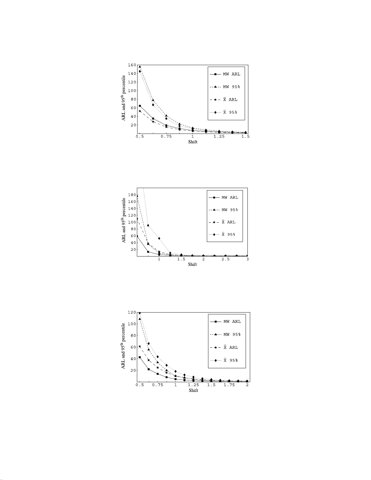
IMS Collectio ns Beyond P arametri cs in In terdisciplinary Research : F estsch rift in Honor of Professor Pranab K. Sen V ol. 1 (20 08) 156–172 c  Institute of Mathematical Statistics , 2008 DOI: 10.1214/ 193940307 000000112 A nonparametric con trol c hart based on the Mann-Whitney statistic Subhabrata Chakra b orti 1 and Mark A. v an de Wiel 2 University of Alab ama and V rije Universiteit Amster dam Abstract: Nonparametric or distribution-fr ee c harts can be useful in statisti- cal pro cess con trol problems when there is limited or l ac k of knowledge about the underlying pro cess distribution. In this paper, a phase I I Shewhart-t ype c hart is considered for lo cation, based on reference data from phase I analysis and the we ll-known Mann-Whitney statistic. Con trol limi ts are computed us- ing Lugannani-Rice-saddlepoint, Edgew orth, and other appr o ximations along with Monte Carlo estimation. The deriv ations tak e accoun t of estimation and the dep endence f rom the use of a reference sample. An illustrative numeri- cal example is presente d. The in-control perform ance of the prop osed chart is sho wn to be muc h sup erior to the classical Shewhart ¯ X ch art. F urther com- parisons on the basis of some per cen til es of the out-of-control conditional run length distribution and the unconditional out-of- con trol ARL show that the proposed chart is alm ost as go o d as the Shewhart ¯ X c hart for the normal distribution, but is more pow erf ul for a heavy-tailed distribution suc h as the Laplace, or f or a skew ed dis tribution such as the Gamma. In teractiv e soft- wa re, enabling a complete implement ation of the chart, is ma de a v ailable on a we bsite. 1. In tro ductio n Control charts are most widely used in sta tistical pro cess co ntrol (SPC) to detect changes in a pro duction pro cess. In conv entional SP C, the pattern of chance causes is often assumed to follow the normal distribution. It is well recognized how ever that in many applications the underlying pro cess distribution is not known sufficient ly to assume nor mality (or any other parametric distribution), so that statistical pro p- erties of commonly used charts, designed to p erform b est under the assumed dis- tribution (such a s normality), could b e p o ten tially (highly) affected. In situations like this, developmen t and application of control charts that do not depe nd on no r- malit y , or m ore generally , on any sp ecific parametric distributional a s sumptions, seem highly desirable. Distribution-free o r no nparametric control charts can serve this purp ose. Chak r ab orti, V an der Laan and Ba k ir [ 4 ] (herea fter CVB) presented an extensiv e overview of the litera ture on univ ariate nonpar ametric control charts. In-control (stable) properties of these c harts are completely det ermined (kno wn) ∗ Supported in part by a su mmer research gran t from the Uni v ersity of Alabama and by a grant from the Thomas Stieltjes Institute for Mathematics. 1 Departmen t of Information Systems, Statistics and M anagemen t Science, Universit y of Al - abama, T uscaloosa, Alabama, USA, e-mail: schakrab @cba.ua.e du 2 Departmen t of Mathematics, V rije Universiteit Amsterdam, Amsterdam, The Netherlands, e-mail: mark.vdw iel@vumc. nl AMS 2000 subje ct classific ations: 62G30, 62-07, 62P30. Keywor ds and phr ases: ARL and run length p ercentiles, conditioning metho d, dis tr ibution- free, Mon te Car lo estimation, parameter estimation, phase I and phase II, saddlep oint and edge- wo rth approximations, Shewhart ¯ X chart, statistical pro cess con trol. 156 Contr ol chart b ase d on the Mann-Whitney statistic 157 and remain the same for all contin uous distributions and hence their out-o f-control behavior are more meaningful and comparable. In this pa p er we use the well-known Mann-Whitney test statistic as a charting statistic for detecting lo cation shifts. The pro blem o f monitoring the center or the lo cation of a proces s is important in many applications. The lo cation par a meter could b e the mea n or the median or some p er cent ile of the distribution; the latter t wo ar e often more attractive when the underlying pro ce s s distribution is exp ected to b e skewed. Among the av aila ble control charts for the mea n of a pro cess, the classical Shewhart ¯ X chart is the most p opular beca use of its inherent simplicit y and practica l a ppea l. In so me a pplications, the pr o cess distribution and/or the parameters are sp ecified or can b e a s sumed k nown. This is typically referr ed to as the sta nda rds known cas e (Montgomery [ 11 ], pa ge 228). If on the other ha nd the parameters are unknown and are estimated from data, there is growing evidence in the recent litera ture that mos t standard charts, including the Shewhart ¯ X chart, behave quite p o o rly in terms of the fa lse alar m ra te a nd the average r un length. W e do not a ssume that the pro cess parameters are sp ecified or that the pr o cess distribution is kno wn, instead, we assume that a reference sa mple is av ailable from the in-co n trol pro cess fro m a phase I ana ly s is. Once the control limits are deter mined from the reference sample, monitoring of test samples is begun. This is referred to as a phase I I a pplication. There a re some phase I I nonpa rametric charts av a ilable in the litera ture; the reader is re fer red to CVB for many re fer ences and detailed acc ount s. The non- parametric charts considered by Cha krab orti, V a n der Laa n and V an de Wiel [ 5 ] (hereafter CVV) are based on the precedence test. It is s een tha t the precedence charts are g o o d alternatives to the ¯ X chart in some situations. How ever, while the precedence charts are a step in the right dir e c tio n, it is known that the nonpara- metric test underlying this chart, the pr ecedence test, is neither the most p ow er ful test (for lo cation) nor the mo s t commonly used nonparametric test in pra ctice. With this motiv ation, we consider a chart based on the p opular and more p ow e r ful Mann-Whitney [ 9 ] (hereafter MW) test which is equiv a lent to the p erha ps mo r e familiar Wilcoxon [ 15 ] rank-sum test. This is c a lled the MW co n trol chart. One might susp ect that the distribution-free-nes s of the MW chart might come at a “los s of p ow er” with resp ect to parametric charts. How ever, remark ably , even when the underlying distributions ar e normal, the MW test is ab out 9 6% as ef- ficien t (Gibbons and Chakrab or ti [ 7 ], pag es 278– 279) as (the mo st efficient) t-test for mo dera tely large sample sizes, a nd yet, unlik e the t-test, it do es not require nor- malit y to b e v a lid. Park and Reynolds [ 12 ] realized the p otential o f no nparametric control charting and intro duced a chart based on this s tatistic. They considered v arious prop erties of this chart when the refer e nce sample size approaches infinit y , which essentially amounts to assuming the sta nda rds known cas e. While this is impo r tant for theoretical purp os e s a nd gives some insight, such a chart do es not app ear to b e very useful in practice where par ameters a nd/or the under lying dis- tribution are unknown a nd need to b e estimated from a moder ate size phase I data set. In fac t, it is cr ucial to develop and implement the MW chart in pr a ctice for small to mo der ate reference sample s izes since, as we show la ter in the pap er, the MW c hart can be esp ecia lly useful in such cases. While the principles of this chart are s imple, practical implemen tatio n o f the chart, i.e., developing an efficient algorithm for computing the co nt rol limits, re - quires s o me effort. W e provide softw are for practical use o f the c hart. Effectiveness of the chart is examined on the basis of several in-co nt rol and out-o f-c o nt rol p er- formance criteria . W e conclude with a discussion, including some topics for further 158 S. Chakr ab orti and M. A. van de Wiel research. 2. The MW con trol c hart Suppos e that a re fer ence sample o f size m , denoted by X = ( X 1 , . . . , X m ), is av ail- able from an in-co nt rol pro cess a nd that Y = ( Y 1 , . . . , Y n ) denotes an arbitra ry test s a mple of size n . The sup ersc r ipt h is used to deno te the h th test s a mple, Y h = ( Y h 1 , . . . , Y h n ) , h = 1 , 2 , . . . , when necessary for notational clarity; otherwise, the supers cript is s uppr e s sed. Ass ume that the test samples are indep e ndent of eac h other and are all indep endent of the r eference sample. The MW test is ba sed on the total num b er of ( X , Y ) pairs wher e the Y observ ation is larger than the X . This is the statistic (2.1) M X Y = m X i =1 n X j =1 I ( X i < Y j ) = n X j =1 { I ( Y j > X 1 ) + · · · + I ( Y j > X m ) } , where I ( X i < Y j ) is the indicator function for the even t { X i < Y j } . Note that M X Y lies (attains v alues) b e tw een 0 a nd mn and large v alues of M X Y indicate a po sitive shift, whereas small v alues indicate a negative shift. The pr op osed tw o- sided MW ch art us es M h X Y as the charting statistic, whic h is M X Y for the h th test sample. The chart signals if M h X Y < L mn or M h X Y > U mn , where L mn and U mn are the low er co nt rol limit (LCL) and the upper control limit (UCL), res p ectively . The distribution of M X Y is known to be sy mmetric ab out mn/ 2 when the pro cess is in-co nt rol, so it is rea s onable to take L mn = mn − U mn . W e fo cus on t wo-sided charts, one-s ided charts can b e developed similarly . 2.1. D esign and implementation Implemen tation of the chart r equires the co n trol limits. Typically , in pra ctice, the co nt rol limits are determined for some sp ecified in-control av erage r un length ( ARL 0 ) v alue, say 370 o r 500. If the successive charting s ta tistics M 1 X Y , M 2 X Y , . . . corresp onding to test sample 1 , 2 , . . . were indep endent, then, as in the sta nda rds known case, the ARL 0 would b e eq ua l to the recipro cal of the false alar m rate, p 0 = 2 P 0 ( M X Y > U mn ), where the subscript 0 deno tes the in-control case. So if the charting statistics were indep endent , the uppe r control limit U mn would b e e qual to the tw o- sided critical v alue for a MW test with size equal to 1 / AR L 0 . Howev er, such critical v alues are not exp ected to b e found in av aila ble tables for the MW test, since in a typical control charting application ARL 0 = 37 0, which means that the UCL i s the upp er critical v alue for a MW test with size 1 / 2 (1/370 ) = 0.00135 . Even if such cr itica l v a lues could b e found, the main pro blem with their use is that the successive charting statistics M 1 X Y , M 2 X Y . . . are dep endent, since the test samples are all compared to the same control limits derived from the same reference sample, and this dependence affects a ll op eratio na l a nd p erformance characteristics of the c o nt rol chart, s uch as the false alar m rate, the AR L , etc. (see, for exa mple, Quesenberry [ 13 ] and Chak r ab orti [ 3 ] for the Shewhart ¯ X chart). It might b e arg ued that for “large” amoun ts of reference data suc h dep endence ca n b e ig no red. There are tw o problems with this argument, how ever. One, we would need to k now the size Contr ol chart b ase d on the Mann-Whitney statistic 159 of the reference data, a -priori, that w ould supp ort ig noring dep endence, and t wo, we would hav e to wait muc h lo nger to gather that amount of data while pro cess monitoring has to wait, costing time a nd money . The solution to this is the ability to calcula te the control limits for any given (fixed) m a nd n and ARL 0 in a given situation. T o this end we first develop an efficient metho d to calculate the ARL . 2.2. C alculation of the ARL Let F and G r e pr esent the cdf of X and Y resp ectively , and suppos e that F and G are contin uo us , s o that “ties” betw een the X ’s and the Y ’s, as well as within the X ’s and the Y ’s can b e ignored theoretically . It is conv enient to der ive the ARL by conditioning on the reference sample, i.e. using the so-c alled conditioning metho d. T o this end, o bserve that the probability o f signal for any test sample, g iven the reference sample X = x , is (2.2) p G ( x ) = P G ( M xY < mn − U mn ) + P G ( M xY > U mn ) . Let N denote the run length r andom v ariable for the chart. Given the refere nce s a m- ple X = x , and that tw o a rbitrary test samples Y h and Y l , ( h 6 = l ) ar e indep endent, which implies the indep endence of M h xY and M l xY . Hence, (2.3) ARL = E ( N ) = E F [ E G ( N | X = x )] = E F ( 1 p G ( x ) ) = ∞ Z −∞ · · · ∞ Z −∞ 1 p G ( x ) dF ( x 1 ) · · · dF ( x m ) = ∞ Z −∞ · · · ∞ Z −∞ ν ( G ( x 1 ) , . . . , G ( x m )) dF ( x 1 ) · · · dF ( x m ) , say . The seco nd equality in ( 2.3 ) follows from a pro pe r ty o f exp ectation. The third equality follows since g iven X = x , N is geometrically distributed with par ameter p G ( x ). The fourth equality is o btained by writing 1 / p G ( x ) as a function o f G and x 1 , . . . , x m , s ay , ν ( G ( x 1 ) , . . . , G ( x m )) = ν ( P G ( Y j < x 1 ) , . . . , P G ( Y j < x m )) , where ν is some function. This can b e done since p G ( x ) is a sum of pro ba bilities like P G ( M xY = u ) , which, in turn is a s um of pro ba bilities ov er all config ur ations of the x ’s and Y ’s for which M xY equals u . Naturally , the proba bilit y o f s uch a configuration only depends on G ( x 1 ) , . . . , G ( x m ) . The (unconditional) ARL of the chart is the mean (exp e c ta tion) of the distribu- tion of the random v ariable E G ( N | X ), which is the conditional average run length, given the random re ference sample. P ercentiles of the distribution of E G ( N | X ) (and not just the mean) are useful to study a nd ch aracter ize control chart p erformance when parameters are estimated, and we develop efficient algorithms to compute these. First how ever, w e fo cus on the mean of the conditional distribution, that is the unconditional ARL giv en in (2.3), when the pr o cess is in-con trol. In the in-co nt rol situation the X ’s and the Y ’s co me from the same distribution 160 S. Chakr ab orti and M. A. van de Wiel F = G . Therefor e, we ma y ass ume w.l.o .g. that F = U [0 , 1 ]: (2.4) ARL 0 = ∞ Z −∞ · · · ∞ Z −∞ ν ( F ( x 1 ) , . . . , F ( x m )) dF ( x 1 ) · · · dF ( x m ) = 1 Z 0 · · · 1 Z 0 ν ( u 1 , . . . , u m ) du 1 · · · du m = 1 Z 0 · · · 1 Z 0 1 p U ( u ) du 1 · · · du m , where p U ( u ) = P U ( M uY < m n − U mn ) + P U ( M uY > U mn ) is the co nditional probability o f a signal at any test sample, given the reference sample u , when the pro cess is in-control. The subscript U is used to deno te that in the in-control case b oth the reference and the tes t samples can be thought of coming fro m the same distribution, the U [0 , 1] distribution, which shows that the in-control ARL of the prop osed chart do es not dep end on F . The same a rgument can b e used to show that the in-control run-length distribution do es not dep end on F and hence the pr o p osed chart is distribution-free. W e emphasize that for the in-control case, without any lo s s of generality , the co mmon ( F = G ) distribution can b e assumed to be the U [0 , 1 ] distribution by virtue of the probability integral transform (see, for example, Gibb o ns and Chakrab orti [ 7 ]). This simplifies calculations co nsiderably . W e need to calculate (2.4) to implement the chart and ( 2.3 ) to ev aluate chart per formance. F or both of these ob jectives there are tw o problems. First, an e x plicit formula for p G ( x ) (or p U ( u )), is not known, which preven ts a direct computation. Second, we have an m -dimensional int egration in bo th ( 2.3 ) and ( 2.4 ). Our approa ch is to calculate p G ( x ) (and p U ( u )) (exactly or approximately) using a fast algorithm, and then use that to a pproximate the integral in b oth ( 2.3 ) and ( 2.4 ) with a Mon te Carlo estimate to get estimates (2.5) A ˆ RL G ≈ 1 K K X i =1 1 p G ( x i ) and (2.6) A ˆ RL 0 ≈ 1 K K X i =1 1 p U ( u i ) , where x i. = ( x i 1 , . . . , x im ) is the i th Monte Car lo s ample, i = 1 , . . . , K , of which each comp onent is drawn from so me sp ecified F for the A ˆ RL G , and K denotes the n umber of Monte Car lo samples used. Similarly , for the in-control situation, u i is a Mon te Car lo sample from U [0 , 1]. F or an a ccurate a pproximation, K needs to be sufficient ly large and ther efore a fast metho d of computing the signa l proba bilit y p G ( x ) (a nd p U ( u )) for an arbitra ry reference sample x is essential for the pra c tical use of the approximation. The ARL calculatio ns pro cee d in tw o steps. The firs t step is to find a fast and efficient metho d to c o mpute the signa l pro bability . W e detail the pro cedure for fast computation of p G ( x ); calculation o f p U ( u ) is similar. Contr ol chart b ase d on the Mann-Whitney statistic 161 2.3. F ast c omputation of signal pr ob abili ty F rom ( 2.1 ) it is s een that the MW statistic is the sum P n j =1 C j , wher e C j repre- sents the num b er of X ’s that a r e less than an Y j . F r om ( 2.2 ) it follows that the calculation of p G ( x ) essentially requir es ca lculation o f the upp e r -tail probability P G ( M xY > U mn ), say , a nd this in turn requires (i) efficient enumeration o f all n - tuples { C 1 , . . . , C n } for which the sum is gr eater than U mn and (ii) summation o f the probabilities for suc h tuples. Note that P ( C j = l ) is eq ua l to P ( X ( l ) < Y j < X ( l +1) ), wher e X ( l ) denotes the l th ordered obser v a tion in the refere nce sa mple for l = 1 , . . . , m with X (0) = −∞ and X ( m +1) = ∞ , say . Given the refer ence sample, the la st pr obability is simply P ( x ( l ) < Y j < x ( l +1) ), whic h is denoted by a l , l = 0 , . . . , m . Also, given the reference sample, no te that the r a ndom v ariables C j are i.i.d. Hence the conditional probability genera ting function (pgf ) of C j is (2.7) H 1 ( z ) = m X l =0 P ( C j = l ) z l = m X l =0 a l z l . Again, since given the refer e nce sample the C j are i.i.d., the conditional pgf of M xY (the sum of the C j ), is simply the pr o duct of the pg f ’s in ( 2.7 ) (2.8) H 2 ( z ) = mn X j =0 P ( M xY = j ) z j = ( m X j =0 a j z j ) n . In principle, P G ( M xY > U mn ) can be calculated by ex panding the power in ( 2.8 ) and collecting the co efficient s o f all terms with degree greater than U mn . Howev er, for moder ate to large m (say , m ≥ 1 0 0) and n not very small (say , n ≥ 5) this takes a considerable amount of co mputing time, esp ecially s ince the pro cedure ha s to b e rep eated K (a large num b er) times, o nce for each Monte Carlo sample. Alterna tive, faster, methods such as “a branch-and-bo und” a lgorithm, based on Mehta et al. [ 10 ] can be used to shorten the intermediate expr essions that result from expanding ( 2.8 ) and sav e s considerable time. How ever, even with the bra nc h-and-b ound algo r ithm, m and n mig ht be just to o large to allow for exact computations and hence a go o d approximation to the co nt rol limits may b e necessary . F or example, we may apply the central limit theorem for the sum o f i.i.d. random v ariables to M xY = P n j =1 C j to get a norma l approximation to P G ( M xY > U mn ) but in our context, U mn is t ypically far in the upper tail of the distribution of M xY and n is usually not very larg e, and so the normal approximation is not very accura te. Instead, we find the Lug annani-Rice for m ula (hereafter LR-formula; see Jensen [ 8 ], page 74) for the upp er-tail pro ba bilit y for the mean of i.i.d. discrete random v a riables (whic h is a “ saddlep oint” approximation formula) to b e particula r ly useful. This formula is known to b e mor e a ccurate than the nor mal approximation in the tails of a distribution and is based on the cumu lant generating function of C j , which is obtained from the pgf in (2.7): k ( t ) = lo g[ H 1 ( e t )]. Let m ( t ) a nd σ 2 ( t ) denote the firs t and the s econd deriv ative of k ( t ), resp ectively . F urthermore, let u = ( U mn + 1) /n and ¯ M xY = M xY /n . The saddlep oint γ is the solution to the equation m ( t ) = u . Using (3.3.17 ) in Jensen (1995 , page 7 9) we obtain P G ( M xY > U mn ) = P G ( ¯ M xY > U mn /n ) = P G ( ¯ M xY ≥ u ) (2.9) ≈ 1 − Φ( r ) + φ ( r )( 1 λ − 1 r ) , 162 S. Chakr ab orti and M. A. van de Wiel where λ = n 1 / 2 (1 − e γ ) σ ( γ ) , r = ( sg nγ ) { 2 n ( γ u − k ( γ )) } 1 / 2 , Φ( . ) and φ (.) are, r esp ectively , the cdf and the pdf of the s ta ndard normal distribu- tion. Using ( 2.9 ), we can efficiently approximate the signal pro babilit y p G ( x ) given in ( 2.2 ). 2.4. Monte Car lo estimation of ARL and err or c ontr ol F rom formulas ( 2.5 ) and ( 2.6 ) we observe that the computation of p G ( x ) is rep e a ted many times to o btain a Monte Car lo approximation of the A RL . The question here is reg arding K , the num b er o f samples so that the Mon te Carlo err or is acce ptably small. Since, fo r the purp ose o f ARL computation, the r eference samples are drawn independently from G (or U [0 , 1] in ca se o f AR L 0 ), the Monte Carlo standard error is estimated by s mc = s ( ARL G ( X )) / √ K , where s (.) denotes the sample sta ndard deviation computed from K s im ulated reference samples. Then, we may choose the smallest K such that (2.10) s mc = s ( ARL G ( X )) . √ K ≤ D , where D is either a sp ecified num b er or a perc e ntage of the current estimate A ˆ RL G . W e can start with say K = 100 , increas e K , compute s mc , and rep eat the pro cess un til the spe cification s mc ≤ D is met. Use o f formula ( 2.10 ) provides a way to obtain an efficient a nd a rea sonably accura te approximation to ARL G . Asymptotic probabilistic control o f the accur acy may b e achi eved b y using the no rmal distribu- tion for A ˆ RL G . F o r example, one could set D such that the proba bilit y that A ˆ RL G deviates mor e than C units from the real mean is smaller than 0 . 05. Here, C could be a small p er cent age of the curr ent estimate. Next, we discus s the approximation of ARL 0 in more detail. Appr oximation of ARL 0 Three metho ds of approximating ARL 0 hav e been introduced so far , each base d on a different metho d to compute or approximate p U ( u ). T o summarize, they are: 1. Exact (EX): Monte Carlo sim ula tion using ( 2.6 ), with p U ( x ) co mputed ex actly using formula ( 2.8 ) 2. LR-for mul a (LR): Monte Carlo simul ation using ( 2.6 ), with p U ( u ) computed approximately using formula ( 2.9 ) 3. Norma l (NO): Monte Carlo simulation using ( 2.6 ), with p U ( u ) computed from a normal approximation W e compare these methods on the basis of acc ur acy a nd sp eed. While s e tting a v alue of D , we observed that K was usually under 100 0, and the maximum Monte Ca r lo error was 2% of the tar get ARL 0 = 500 , that is, e q ual to 10. The v alue o f K was set to 100 0 and kept unchanged in these computations to get a fair co mparison of the computing times. Mor eov er , we intro duce tw o a lternative methods to calculate ARL 0 : 4. Fixed reference sample (FR): Fix r eference sample to q = (1 / ( m + 1 ) , . . . , m/ ( m + 1)) and approximate ARL 0 b y 1/ p U ( q ) 5. 1 /(false ala rm rate) (F A): a ppr oximate AR L 0 b y the recipro cal of the false alarm rate: 1 / (2 P 0 ( M X Y > U mn )). Contr ol chart b ase d on the Mann-Whitney statistic 163 T able 1 ARL 0 appr oximations and c omputing times EX LR NO FR F A A ˆ RL 0 time A ˆ RL 0 time A ˆ RL 0 time A ˆ RL 0 time A ˆ RL 0 Time m n (sec.) (sec.) (sec.) (sec.) (sec.) 50 5 486 54 506 36 307 1.0 403 0.05 247 0.01 10 504 395 505 34 327 1.0 524 0.05 226 0.01 25 488 4850 491 31 425 1.2 694 0.05 119 0.01 100 5 496 220 505 48 219 1. 2 478 0.05 353 0.01 10 505 1920 506 47 339 1.3 531 0.05 332 0.01 25 ** 26168 503 48 422 1.3 683 0.06 233 0.01 500 5 491 10633 496 207 226 1.2 492 0.20 445 0.01 10 ** 73516 513 179 367 1.7 537 0.21 484 0.01 25 ** 7.59*10 5 494 176 445 1.6 578 0.29 450 0.01 1000 5 ** 31766 500 356 235 2.1 513 0.48 471 0.01 10 ** 3.42*10 5 499 373 355 2.4 516 0.49 488 0.01 25 ** 3.15*10 6 500 348 442 1.7 548 0.63 482 0.01 2000 5 ** 1.71*10 5 503 713 234 2.1 506 0.67 474 0.01 10 ** 1.44*10 6 504 659 354 1.9 513 0.71 499 0.01 25 ** 1.29*10 7 509 676 446 2.1 531 1.41 497 0.01 ∗∗ ARL 0 could not reliably b e estimated wi thin reasonable time; computing time f or K = 1000 is obtained by multiplying computing time for K = 1 b y 1000 (sampling algori thm is linear in K ). Let us expla in a ppr oximations 4 and 5. When m is large, the empirical cdf F m ( x ) conv erg es to F ( x ) (which is the cdf of the U [0 , 1 ] distribution) and hence for large m we may approximate the i th reference sa mple o bserv ation by the i/ ( m + 1) th quantile of the U [0 , 1 ] distribution, q i = i/ ( m + 1), i = 1 , . . . , m . Thus, we a pproximate the ARL 0 , for la rge m , by 1 /p U ( q ), wher e q = ( q 1 , . . . , q m ). This is metho d 4. The ma jor benefit with this approximation is that we need to co mpute p U ( u ) only once (namely at u = q ) instead o f K times as needed in methods 1 through 3 fo r each of K Monte Carlo reference s amples. Finally , another quick approximation for the ARL 0 is given b y the in verse of the false ala r m r a te, 1 / (2 P 0 ( M X Y > U mn )). In a setting where runs are truncated at a finite p o int T , the latter approximation was proven to b e un biased when m appro a ches infinit y in Park and Reynolds [ 12 ]. This approximation is metho d 5 . Cha krab orti [ 3 ] show ed tha t for the Shewhar t ¯ X chart, 1/F AR is a low er b ound to ARL 0 and noted that this b ound c an serve as a “quick and dirty” approximation to the ARL 0 for mo derate to larg e v alues of m . When a pplying method 5, we used formula (1 1) in Fix and Ho dges [ 6 ] to c o mpute P 0 ( M X Y > U mn ), based on an Edg eworth approximation, whic h significantly improv es the normal approximation by including moments of or der higher than 2. T able 1 displays the estimated ARL 0 v alues computed b y the fiv e metho ds for fifteen combin ations of m and n . Chart constants were deter mined (using the al- gorithm discussed in the next section) such that AR L 0 ≈ 500 , when applying the exact formula ( 2.8 ) or the b est approximation, the LR-formula, when exact co mpu- tations were to o time-co nsuming. Therefore, the closer an AR L 0 v alue is to 500 , the better the a pproximation. The table als o shows the computing times on a 1.7 GHz Pen tium PC with 128MB of internal RAM. Several observ ations can be made fro m T able 1 . First we see that the “ gold standards” or the exact computations are very time-consuming for most v alues of m and n . Howev er, when they can b e found, they would naturally for m the basis of our compar is ons of v arious approximations. Seco nd w e se e that the nor mal approximation is no t very accur a te, but the LR-a pproximation is, particular ly for m ≤ 100 , n ≤ 10 and for m = 500, n = 5. Since the LR-a pproximation is known to b ecome more accurate when the sample sizes increase, one may safely apply 164 S. Chakr ab orti and M. A. van de Wiel the LR- fo rmula also when m ≥ 50 and n ≥ 5 in order to implemen t the pro p osed chart. It may be noted that when m increa ses, the computing times with the LR– formula also increase, although, b y far , not as dr amatically as the times for the exact computations. This suggests that in practice (for finding the chart cons ta n ts, to b e discussed next) there is still r o om for an alternative, quick approximation of ARL 0 , particular ly fo r large v alues of m . Co mpared to the LR-fo r mul a, we o bserve that both the “ fast” approximations (metho ds 4 and 5) are quite go o d for m ≥ 10 00 and that the fixed reference s ample approximation (metho d 4) per forms somewha t better for relatively small v alues of n ( n = 5 ,10) than for n = 25 . T o summar ize, the b est metho d of ca lc ula ting the ARL 0 is the exa ct EX metho d if it is computationally feasible, otherwise, the b est approximation is the LR meth- o d. In pra ctice, we recommend using the LR-metho d, b ecause it is b oth fast and accurate. If the r eference sample is very lar ge, say m ≥ 100 0, o ne of the t wo faster approximations, either FR or F A, can be used. 2.5. D etermination of chart c onstants Since we can now calculate the ARL 0 corresp onding to a g iven v alue of U mn effi- cient ly and accura tely , we can use an iterative pr o cedure based o n linear in terp ola- tion to find the control limit for a pr e-sp ecified ARL 0 v alue, s ay 500. In principle, we use the LR-a ppr oximation fo r the computation of ARL 0 . How ever, we hav e obser ved that this approximation is still somewhat time-consuming, so w e wan t to minimize the nu mber of iterations for which the LR a ppr oximation is used. T o this e nd a go o d starting v alue of U mn is needed and this is where the fast approximations FR and F A are very useful. Starting with the F A approximation, we simply equate the in verse of the false alarm rate to 50 0, which means so lving 1 / (2 ∗ F H ( u )) = 500 for u in or der to get a n initial guess for U mn . Since the FR approximation is so mewhat better than F A for m ≤ 500 , we use this initial guess with the FR a pproximation to refine the Fix-Ho dges approximation when m ≤ 500 . The r esulting approximation for the U CL is then used as an initial guess for the linear in terp olation metho d with the LR-for mu la. W e do not detail the search pr o cedure here, but illustrate it with a n example. Supp ose that m = 3 75 and n = 7, and we want to find the c hart constants such that ARL 0 ≈ 400. Supp ose we allow a deviation of 2% (whic h is 0.0 2 * 400 = 8) maximally , hence the sea rch pro cedure w ould s top and y ield the desir ed control limit U mn , when 3 92 ≤ A ˆ RL 0 ≤ 40 8. Moreov er, supp ose we stipulate that the Mo n te Car lo standard erro r s mc be smaller than 1.5% o f the curr ent estimate of A ˆ RL 0 ; fro m inequality ( 2.10 ) w e obser ve that this r e quirement determines the n umber of Monte Carlo sa mples K pe r iteration, when setting D = 0.01 5 * 4 00 = 6. The output from our prog ram (written in Ma thematica; see Soft ware section later) is s hown in T a ble 2 . As can b e seen in T a ble 2 , six iterations (num b er ed 1 through 6) hav e b een executed in approximately 1 4 0 seconds. The first three of these hardly take any computing time, b ecause the fast F A and FR approximations w ere used. F or each iteratio n, the v alues of the UCL and the LCL and the corres p o nding ARL 0 are shown. Under the LR metho d, the pro gram also calculates the 5 th per centil e of the co nditional in-control ARL distribution and the Mon te Carlo standar d error ( smc ). Note that the first step with the LR metho d, step 4, uses the chart constants of step 3, which is our b est guess fro m the fa s t a pproximations, as initial v alues. Also, note that for the LR metho d, the first t wo iterations (4 and 5 ) pro duce AR L 0 v alues b elow and ab ove the tar get v alue 40 0, so that linear interpolation beg ins at the third iteration and the new UCL is found using the tw o previous UCL ’s Contr ol chart b ase d on the Mann-Whitney statistic 165 T able 2 Finding c ontr ol limits for m = 375, n =7 and tar get ARL 0 = 400 F A: 1/(fa lse alarm rate) appro xim ation 1. ucl=2146 lcl=479 ARL0=400 FR: Fixed reference sample approximation 2. ucl=2146 lcl=479 ARL0=446.761 3. ucl=2136 lcl=489 ARL0=386.729 LR approximation 4. ucl=2136 lcl=489 ARL0=380.059 smc=5.69018 5% perc=238.407 K=402 5. ucl=2146 lcl=479 ARL0=438.11 sm c=6.5647 5% perc=287.53 K=319 6. ucl=2139 lcl=486 ARL0=394.496 smc=5.91419 5% perc=252.778 K=315 139.962 Second T able 3 L ower and upp er MW c ontr ol c hart limits for sele ct e d values of m , n and ARL 0 ARL 0 = 370 A RL 0 = 500 m n L mn U mn L mn U mn 50 5 35 215 33 217 10 115 38 5 11 1 389 25 400 85 0 39 3 857 100 5 69 431 65 435 10 231 76 9 22 4 776 25 805 1695 793 1707 500 5 348 2152 328 2172 10 1170 3830 1128 38 72 25 4081 8419 4016 84 84 1000 5 698 4302 653 4347 10 2344 7656 2268 77 32 25 8169 16831 8058 16942 2000 5 139 7 8603 1309 8691 10 4682 15318 4540 15460 25 16392 33608 16145 33855 and their corresp onding AR L 0 v alues. Th us, the fina l chart constants are found at iteration 6, U mn = 2139 and hence L mn = 48 6, with attained A RL 0 = 394.5 . The 5 th per centil e o f the conditiona l in-co ntrol ARL dis tr ibution, at this iter a tion, is found to b e 252 .78. So using the MW chart with UCL = 213 9 and LCL = 486 , the unconditiona l AR L 0 = 39 4 . 5 implies that when the pro c e s s is in-control, on an av era ge, a fals e alarm is exp ected every 3 95 s amples. The 5 th conditional p ercentile implies that for 95% of all reference samples (that could have p ossibly b een taken from the in-control pro cess), the av erag e run length is at least 2 53. T able 3 shows chart constants computed with this algor ithm for a num b er of combinations o f m and n . All cas e s are tw o-sided and AR L 0 equals either 37 0 or 500. 2.6. Nu meric al example T able 5.1 in Mo nt gomery [ 11 ] gives a set of data o n the inside diameters o f pisto n rings manufactured by a forging pro cess . Twen ty-fiv e samples, eac h of size five, were collected when the pro cess was thought to be in-control. The traditional Shewhart ¯ X and R charts provide no indication of an out-o f-control c o ndition, so these “trial” limits w ere adopted for use in on-line proc e ss control. F or the pr o p osed MW chart with m = 1 25, n = 5 and ARL 0 = 400 , we find the upp er co n trol limit U mn = 540 and hence the low er co ntrol limit L mn = 85. Having found the c o nt rol limits, prosp ective pro cess monitoring in phase I I b egins. 166 S. Chakr ab orti and M. A. van de Wiel Fig 1 . MW Chart f or the Piston-ring data. Montgomery also g ives (T a ble 5.2) fifteen additional samples from the piston-r ing manuf acturing pro cess. These “test samples” lead to fifteen MW statistics ca lc ula ted using Minitab: 429.0, 33 3.0, 142.5, 37 0.5, 241.5, 410.5 , 3 93.0, 240.5 , 4 71.0, 486.0, 3 4 0.5, 561.0, 575.5, 60 1.5 and 484 .5. Co mparing each sta tistic w ith the co ntrol limits, all but three of the test g roups, 1 2, 1 3 and 14 are declared to b e in-co nt rol. The co ntrol chart is shown in Figure 1 . The conclusion from this c hart is that the medians o f test groups 12, 13 and 1 4 hav e shifted to the r ight in compariso n with the median of the in-con trol distr ibu- tion, assuming that G is a lo ca tion shift of F . It may b e noted that the Shewha rt ¯ X chart shown in Montgomery [ 11 ] led to the same conclusion with resp ect to the means. Of course, the a dv antage with the MW chart is that it is distribution-free, so that rega rdless o f the underlying dis tr ibution, the in-control ARL of the chart is roughly equal to 400 and there is no need to worry ab out (non-) normality , as one m ust for the ¯ X chart. T o see how the MW chart compares with other av aila ble non- parametric charts, w e calcula ted the distribution-free precedence chart (see CVV) for this data. W e found LCL = 73.982 a nd UCL = 74.0 17 fo r the precedence chart, with an attained ARL 0 ≈ 414 . 0 . Consequently , the precedence chart decla res the 12 th and the 14 th groups to b e out o f co nt rol but not the 13 th group, unlike b oth the MW and the Shewhart c ha rt. Comp arison with the Shewhart chart The p erformance of a co nt rol chart is usually a s sessed in terms of its run length dis- tribution a nd certain a sso ciated characteristics, such as the ARL . While following the general no rm in the literature w e e x amine the ARL , given the sk ewed nature of the run length distribution, we also consider tw o other criteria for ev alua ting and comparing the pe r formance o f the MW chart a nd its pa rametric comp etitor, the Shewhart ¯ X chart, in terms of some p er cent iles of the conditional run length dis - Contr ol chart b ase d on the Mann-Whitney statistic 167 tribution. W e believe these criteria provide additional useful information rega r ding chart p erformance, with estimated parameters. T o ens ure a fair compar ison b etw een the MW a nd the Shewha rt ¯ X chart, first, the ¯ X chart is used for the cas e when bo th the mea n and the v a riance are unknown, with parameter s estimated from the reference sample. Second, the c harts are b oth designed to have the same sp ecified ARL 0 . Note that for the ¯ X chart the non- robustness of the ARL 0 with r esp ect to no n- normal in-co n trol distributions is a ma jor c o ncern. This has b een recog nized as a pro blem elsewher e (see e.g. CVV) and is p erhaps one of the imp ortant reasons fo r cons idering a no nparametric chart in practice. Although b oth the conditional and the unconditional distributions provide im- po rtant information reg arding the p erfo rmance of a co nt rol chart, we ar gue that the conditional distribution migh t be preferred from a practical p oint of view since the unco nditional distribution is what results after “averaging” ov er all p ossible reference s amples. Users would most likely not hav e the benefit of av eraging in a particular application. Also, since the distribution is skew ed, the p ercentiles a nd not the av erage are better measur es of p erformance and thus the standar d deviation app ears to b e a less suitable mea s ure of v ariability . First we consider the in-control case. 2.7. In-c ontr ol p erformanc e F or the in-co nt rol situation, a low er order p e r centile (say the 5 th ) is more useful and rela tiv ely large v a lues of this p ercentile are des irable (in the same s pir it that the ARL 0 of a chart b e large), since that would lead to a smaller probability of a false ala rm. W e a lso show the estimated standard devia tions to g ive an indicatio n of the v aria bilit y of ARL 0 ( X ) , since this a ppea rs to b e the current nor m. F or completeness, the 95 th per centil e is also given. The t wo percentiles can a lso provide an indication of the v ariability in the conditional distribution. The prop osed MW chart for lo cation for is compar ed to the Shewhart ¯ X chart with estimated parameters. There may be some interest in comparing a gainst other control charts and we co mmen t o n this a sp ect later. T o ensur e a fair compar ison, chart cons ta n ts were deter mined such that the ARL 0 approximately equals 500 for bo th ch arts. W e kept the test sample size constant, n = 5, and used several v alues for the r eference sample size m . Bo th samples were drawn from a Normal(0,1) distribution. The num b er of sim ulations, K , was set to 1 000. The results are shown in T able 4 . T o illustrate, suppo se m = 75 0 . While applying the MW chart with U mn = 32 58, from T a ble 4 we know that 9 5% of the in-control ARL ’s (for a large n um b er o f ref- erence samples taken from the in-co nt rol pro cess) will b e at least 360. This provides useful p erfor mance infor ma tion in addition to saying that the unco nditional A RL 0 is 50 0. F o r the ¯ X chart with m = 750 a nd a control chart co nstant of 3.0 89 (this guarantees ARL 0 = 50 0 when parameters are b oth unknown), the 5 th per centil e is 314 so that 95% of the in-control ARL ’s are at leas t 3 14. Since the in-control 5 th per centil es for the MW chart are considerably larger than those of the Shewha r t chart for all m , we conclude that the in-control pe rformance of the MW chart is su- per ior to that of the Shewhart chart with estimated limits, particularly for m ≤ 15 0. Thu s the MW chart is more useful in applications where a larg e amount of refer- ence data might not b e av aila ble. The uniformly smaller standard deviations for the MW chart doubly co nfirm its supe r iority . No te a lso that a s m increas es, b oth the 168 S. Chakr ab orti and M. A. van de Wiel T able 4 Fifth and ninety- fifth p e rc enti les and st andar d deviations of the co nditional in-co ntr ol distribution of ARL 0 ( X ) ; Al l c ases: n = 5 and ARL 0 = 500 Upp er Upp er c ontr ol 5 th 95 th St. c ontr ol 5 th 95 th St. limit p er c. p er c. Dev. limit p er c. p er c. Dev. m MW MW MW MW Shewhart Shewhart Shewhart Shewhart 50 217 97 1292 553 3 . 01996 49 1619 854 75 326 146 1219 461 3 . 0515 6 87 1379 645 100 435 182 1146 358 3 . 06535 112 1290 463 150 654 251 1090 315 3 . 07715 154 1197 377 300 1304 284 845 197 3 . 08607 232 9 27 235 500 2172 322 700 140 3 . 08848 270 8 28 174 750 3258 360 677 107 3 . 08935 314 7 65 140 1000 4347 379 674 83 3 . 08969 338 7 21 121 1500 6520 409 642 71 3 . 08996 367 6 78 97 2000 8691 420 629 55 3 . 09007 376 651 84 5 th as the 95 th per centil es approa ch the mea n o f the corr esp onding unconditional distribution, the ARL 0 , which is set at 5 0 0. 2.8. O ut-of-c ontr ol p erformanc e The distribution- fr e e prop erty (and the resulting r obustness of the ARL 0 ) is an im- po rtant asset of the pr op osed c hart, but wha t ab out its out-of-control p erfor mance? W e address this issue her e. Since this is a chart for lo cation, our interest is in the shift (lo cation) alternative G ( x ) = F ( x − δ ), where δ is the unknown shift parame- ter. T o study the effects o f using a reference sample, again, we use co nditioning and study the dis tr ibution o f the c o nditional ARL . Let ARL δ ( X ) = E F ( x − δ ) ( N | X ), denote A RL of the run-length distribution, given the reference sample X , when the pro cess distribution F ha s shifted b y an amount δ . W e examine the out-of-control per formance of b oth the MW chart and the Shewhart chart in terms of ARL δ ( X ) next. W e also provide a more tra ditional chart comparison by examining the out-o f- control unconditional AR L for a sp ecified distribution and shift, ARL δ . Naturally , small v alues of ARL δ are des irable. As in the case of the in-control situatio n, we also exa mine a p ercentile of the out-of-control distribution. How ever, in the o ut- of-control ca s e it ma kes sense to fo cus on a higher order p ercentile, s ay the 95 th per centil e. Denoting this by q 0 . 95 , relatively smaller v alues o f q 0 . 95 are desira ble for a preferred chart, since the probability o f a signal is desired to b e hig her in the out- of-control cas e . F or a given v alue of q 0 . 95 , users ca n b e 95% confident that for their own sp ecific r eference sample, the out-of-control ARL is smaller than that v alue. The tw o per formance measures, namely the ARL δ and the q 0 . 95 , are examined for three distributions: Normal, La pla ce and Gamma(2 ,2). The Laplace distribution is normal-like but with heavier tails, which results in hig her probabilities of extreme v alues. The Gamma(2 ,2) distribution is skew ed and is often used in the SPC lit- erature. W e apply tw o-sided charts to the Norma l and the La place dis tr ibutions and a one-sided chart with an upper control limit to the Gamma(2,2) distribution. The test sample size n is 5 a nd the re fer ence sample siz e m is 10 0. Co nt rol limits for b oth the MW chart and the Shewhart ¯ X chart with estimated parameters are determined such that A RL 0 = 500. Using these limits ARL δ ( X ) and the 95 th per - cent ile of the distribution of ARL δ ( X ) are computed for several v alues of δ , which is given in units of the standard deviation. Figures 2 thr o ugh 4 show the results. Contr ol chart b ase d on the Mann-Whitney statistic 169 Fig 2 . Performanc e for MW chart and Shewhart chart under Normal shift alternatives. Fig 3 . Performanc e for MW chart and Shewhart chart under L aplac e shift alternatives. Fig 4 . Performanc e for MW chart and Shewhart chart under Gamma(2,2 ) shift alternatives. 170 S. Chakr ab orti and M. A. van de Wiel F or the set o f po ints, tria ng les and diamo nds, obser ve that for the normal distri- bution the 95 th per centil es for the Shewhart ¯ X chart are all smaller than those for the MW chart. Thus, as one might exp ect, the ¯ X chart is more effective in detect- ing shifts than the MW chart in case of the normal alternative. How e ver, note that the differences b e tw een the p ercentiles are sma ll at all shifts (the la rgest difference is a round 15) and the difference a ppea rs to v a nish for shifts greater than 1. The same pattern holds for the tw o ARL ’s. On the o ther hand, Figure 3, for the Laplace distribution, shows that the MW chart is clear ly b etter than the Shewhar t chart for a ll s hifts, lar ge and small. F o r the Gamma(2 ,2) distribution, in Figur e 4, aga in, we see that the MW c hart is better in detecting s hifts, although the difference in per formance is not as dr amatic as in the case of the Laplace distribution. These calculations were repea ted for m = 500 observ a tions; the results were v ery similar and a r e therefore omitted here. W e co nclude that the nonpar ametric MW chart follows the well-known results for the MW test statistic: it is nearly as effective as the Shewhart ¯ X chart under nor mality , but is more effective under heavy tailed and skew ed distributions. Also, no te that p erfor mance of the MW chart in the c a se of the La place distribution makes it p otentially useful when outliers in the data are not uncommon. 3. Discussions and further topics Comp arison with CUSUM and EWMA charts Shewhart charts are known to b e very go o d for mo derate to lar ge shifts. These charts do not require tuning par ameters lik e those needed b y the CUSUM a nd the EWMA charts for a s pecified shift, but a im for global per formance. Thus although one can design a CUSUM or an EWMA chart to p erform b etter by fo cusing on either small, medium or lar ge shifts, a prior i, the same path could lead to a worse per formance for other shifts. Mo r eov er , a s ha s b een noted in the literature Que- senberry [ 14 ], the very nature and pr inciple of the “ av er ages-type” charts (such as CUSUM and EWMA) is different from that of Shewhar t charts. In addition to the pr oblem of having different in-control run-length distributions that r enders the sta ble pr op erties o f these ch arts to b e quite differen t (and hence out-of-co nt rol assessments less mea ningful), the averages charts are mor e p owerful in detecting sp e c ific t yp es of shifts (sustained monotonic). Nevertheless, w e made an attempt to compare the MW chart with EWMA and CUSUM on the basis of in-co nt rol robustness in terms of misspecifica tions of the shap e of the distribution and the v ariance. Ra ther than showing all the r esults, we summarize the findings here. F or fast detection of large shifts (say 1 and larger), the MW chart is very go o d: it is p ow erful and maximally robust against misspeci- fications o f shap e and v ariance. The latter is far from b eing true for CUSUM and EWMA desig ned for detecting la r ge shifts: true AR L 0 could easily b e t wice as la r ge or small as the target ARL 0 in case of skewness, increa sed v ar ia nce or heavy-tails. F or small shifts, the situation is more delicate: the E WMA is a strong comp e titor , since it is often (but not a lways; for example, no t for medium to large shifts in the normal) mo re p ow er ful than the MW chart a nd quite r obust ag ainst misspe cifica- tions of the shap e. This type of r obustness of the EWMA chart w as shown earlier (see e.g. Borror et al. [ 2 ]). How e ver, the EWMA is seen to b e not robust against a missp e c ification of the v ar iance. F or example, a small incr e a se of the v ariance of a normal (from 1 to 1.1 ) lowered the in-control ARL from 500 to 21 5 for an EWMA Contr ol chart b ase d on the Mann-Whitney statistic 171 designed for s ma ll shifts. The ov er a ll co nclusion is that espec ia lly when the in- control v ariance can b e estimated with limited accuracy , the nonparametric charts in general, and the MW chart in particular, is extremely useful in practice, b ecause they do not req uire knowled ge of the underlying v ar iance. Similar conclusions hav e been dr awn in Amin et al. [ 1 ]. Alternative ch art design criteria T able 4 suggests that with estimated para meters, esp ecially for small v alues o f m , it may be useful to use a low er order (say the 5 th ) p erce n tile of the c onditional distribution as a chart design criterion rather than the mean, i.e., the unconditional mean ARL 0 . The design requirement would b e that the p ercentile be at leas t equal to s ome specified large num ber , s uch a s 300. In so me cases one m ight w ant to avoid very short in-co n trol runs in the future, which sug g ests using a lower p ercentile of the in-control distribution of N a nd not that of the co nditiona l distribution o f E ( N | X ). The proba bilit y P 0 ( N ≤ n ) can b e co mputed using similar metho ds as for computation of ARL 0 . Then, for exa mple, if one wants to avoid in-co ntrol runs smaller than 1 00 with a high pro babilit y , say 0.90, we ca n find the control chart limits by solving P 0 ( N ≤ 100) = 1 − 0 . 90 = 0 . 10 , again using a sear ch algorithm. T o facilitate us e of b oth of these chart design criteria we hav e implemented these in the soft ware that we provide with this pap er. Individual’ s chart There is consider able interest in nonparametric charts for individual o bserv ations ( n = 1) since in this case the notion of a pproximate normality via the central limit theorem is not a pplicable. F or n = 1, formula ( 2.7 ) allows for fast exac t computations. The s oft ware ca n b e used to set up s uch a chart. Because of the natural interest in no nparametric individual’s charts, a detailed treatment of this topic will be given in a future pap er. Monitoring disp ersion The disp ersion or sprea d need not b e monitor ed while using a nonpa rametric c o nt rol chart (suc h as the MW chart) under the lo cation mo del. This has be en cited as an adv antage of the nonpar ametric sign c harts by so me author s. How ever, monitor ing the spr ead is a n interesting practical pro blem in a “lo cation-sca le” mo del and we see the po ssibility of designing a chart for sca le (along with that for the lo ca tion) based on so me nonpa r ametric test for sca le, This topic will be considered in a future pap er. App endix: Soft ware In order to suppo rt practica l implementation of the metho ds presented in this pap er tw o t yp es of softw are r e la ted resour ces are pr ovided. First, a Mathematica 4 .2 W olfram [ 16 ] notebo ok is av ailable to ca lcula te (i) the in-control ARL computations any of the five methods (ii) the out-of-co nt rol perfor mance computations, (iii) the control chart constants and (iv) to plo t the MW-control chart for a user-sp ecified data set. Second, we created a website that enables any o ne to apply the pro po sed 172 S. Chakr ab orti and M. A. van de Wiel methodo logy . The MW control chart limits can b e found for the sample s iz e s a t hand for a sp ecified target ARL 0 (or a desired ( q th) p ercentile o f ARL 0 ( X )). Moreov er , the website a llows users to imp or t their own data set and hav e the MW chart drawn. The site can b e r eached via www.win.tue.nl/ ∼ markvdw . The Mathematica notebo ok is av ailable from the same site; it co n tains more pro cedures and a llows for mor e flexible input. User instructions a re av ailable in the noteb o ok and at the website. Ac knowledgmen ts. W e thank Marko Bo on (TU Eindhov en) for a ssistance with the design of the Mann-Whitney con trol chart w ebsite. References [1] A min, R. W., Reynolds, Jr., M. R. and Bakir, S. (1995). Nonpa r amet- ric quality control charts ba sed on the sig n statistic. Comm. Statist. The ory Metho ds 24 1597 –1623 . MR13499 28 [2] Bo rror, C., Montgomer y, D. and R unger, G. (1999). Robustness o f the ewma cont rol c ha rt to non-normality . J. Quality T e chnolo gy 3 309–3 1 6. [3] Chak rabor ti, S. (2000 ). Run leng th, av er age r un length and false alarm ra te of Shewhar t X-bar chart: Exac t deriv ations by conditioning. Comm. Statist. Simul. Comput. 29 61–81 . [4] Chak rabor ti, S. , V an der Laan, P. and Bakir, S. (2001 ). Nonparametric control charts: an ov erv iew and some results. J. Q uality T e chnolo gy 3 3 304– 315. [5] Chak rabor ti, S. , V an der Laan, P. and V an de Wiel, M. (2004 ). A class of distribution-free control charts. Appl. Statist. 53 443 –462 . MR20 7550 1 [6] Fix, E. and Ho dges, Jr. , J. L. (19 55). Sig nificance probabilities of the Wilcoxon test. Ann. M ath. Statist. 26 301 –312 . MR00701 20 [7] G ibbons, J. D. and Chakrabor ti, S. (20 03). Nonp ar ametric Statistic al Infer enc e , 4th ed. Dekker, New Y ork. MR206 4386 [8] Jensen, J. L. ( 1995 ). Sadd lep oint Appr oximations . Oxford Univ. P ress, New Y ork. MR13548 37 [9] Man n, H. B. and Whitney, D. R. (19 47). On a test of whether one of tw o random v ariables is sto chastically lar ger than the other. Ann. Math. Statist. 18 50–60 . MR00220 58 [10] Meht a, C., P a tel, N. and Wei, L. (1988). Co ns tr ucting exact significance tests with restricted randomization rules. Biometrika 75 295 –302. [11] Montgomer y, D. (20 01). Intr o duction t o Statistic al Quality Co ntr ol , 4 th ed. Wiley , New Y ork. [12] P ark, C. and Reynolds, J r., M. R. (1 9 87). Nonparametric pro cedures for monitoring a lo cation parameter based on linear placement statistics. Se quen- tial Ana l. 6 30 3–323 . MR09245 38 [13] Quesenberr y, C. (1993 ). The effect o f sample size on estimated limits for ¯ X and X control c ha rts. J. Q uality T e chnolo gy 25 237–247. [14] Quesenberr y, C. ( 1995 ). Respo nse. J. Quality T e chnolo gy 27 333–3 43. [15] Wilcox o n, F. (1945). Individual co mpa risons by ra nking metho ds. Biomet- rics 1 80 –83. [16] Wolfram, S. (1 996). The Mathematic a b o ok , 3r d ed. W olfram Media, Inc., Champaign, IL. MR14046 96