Measuring Traffic

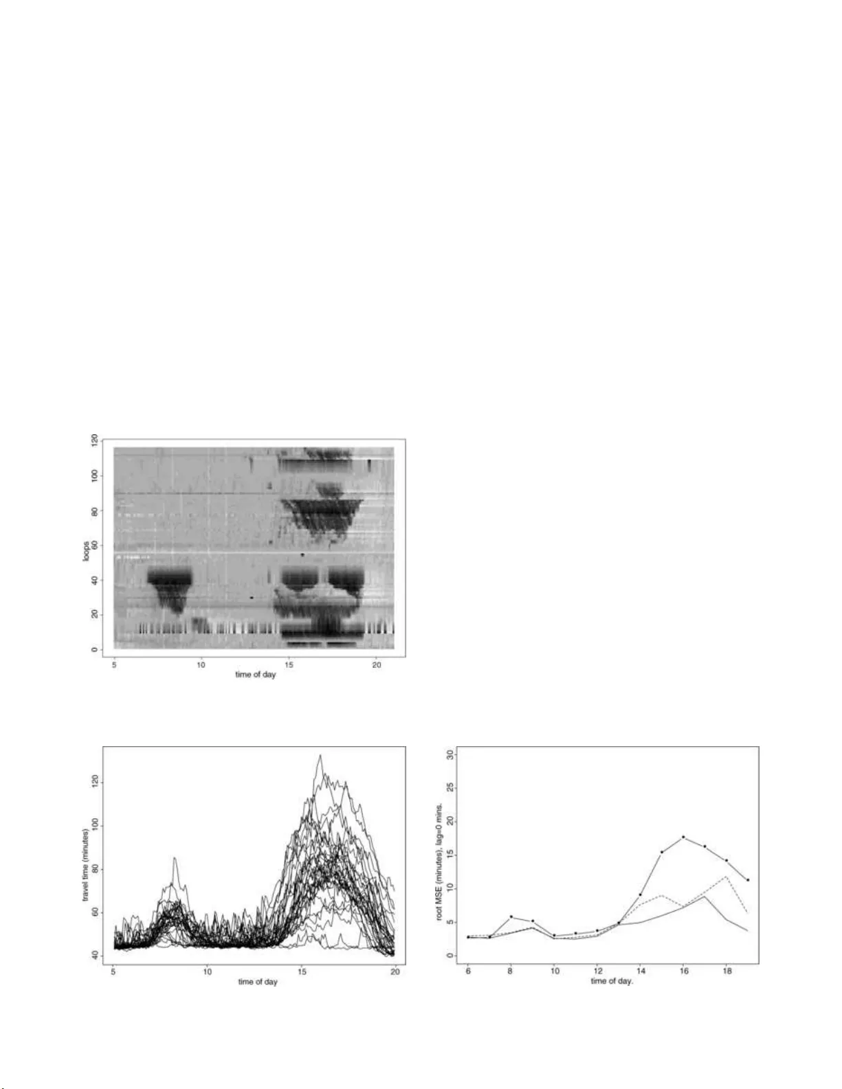
Statistic al Scienc e 2007, V ol. 22 , N o. 4, 581– 597 DOI: 10.1214 /07-STS238 c  Institute of Mathematical Statistics , 2007 Measuring T raffic P eter J. Bick el, Chao Chen, Jaimy oung Kwon, John Rice, Erik van Zw et and Pravin V a raiy a Abstr act. A traffic p erf orm ance mea sur emen t system, PeMS, curren tly functions as a sta tewide rep ository for traffic data gathered b y thou- sands of automat ic sensors. It has in tegrated data collec tion, pro cessing and comm unications infrastructur e wit h data storage and ana lytical to ols. In this pap er, w e discuss statistical issues that ha v e emerged as w e attempt to pro cess a d ata stream of 2 GB p er day of wildly v arying qualit y . In particular, we fo cus on detecting sens or malfunction, impu- tation of missing or b ad data, estimation of vel o cit y and f orecasting of tra v el times on freew a y net w orks. Key wor ds and phr ases: A TIS, freew a y loop data, sp eed esti mation, malfunction d etectio n. 1. INTRODUCTION As v ehicular traffic congestio n has in creased, es- p ecially in u rban areas, so ha v e efforts at dat a co l- lectio n, analysis and mo deling. This pap er discusses the statistical asp ects of a particular effort, the F ree- w a y Performance Mea sur emen t System (Pe MS). W e Peter J. Bi ckel is is Pr ofessor, Dep artment of Statistics, University of Calif ornia, Berkeley, Berkeley, Califo rnia 94720, U S A e-mail: bickel@stat.b erkeley. e du . Chao Chen is a gr aduate student, TFS Capital, 121 N. Walnut Str e et S te 320, West Chester, Pennsylvania 19380 , USA e-mail: chao @tfsc apital.c om . Jaimyoung Kwon is A ssistant Pr ofessor, Dep artment of S t atistics, Califo rnia State U niversity, East Bay, Haywar d, Califo rnia 94542, U S A e-mail: jaimyoung.kw on@csue astb ay.e du . John Ric e is Pr ofesso r, Dep artment of Statistics, U n iversity of Califo rnia, Berkeley, Berkeley, Cali fornia 9472 0, USA e-mail: ric e@stat.b erkeley .e du . Erik van Zwet is with the Mathematic al Institut e, University of L eiden, 2300 RA L eiden, The Netherlands e-m ail: evanzwet@math.leid enun iv.nl . Pr avin V ar aiya is Nortel Networks Distinguishe d Pr ofessor, Dep artment of Ele ctric al Engine eri ng and Computer Scienc e, University of Ca lifornia, Berkeley , Berkeley, California 94720 , USA e-mail: var aiya@e e cs.b erkeley.e du . This is an electronic reprint o f the original ar ticle published by the Institute of Mathematical Statistics in Statistic al Scienc e , 2007 , V o l. 22 , No. 4, 581–5 97 . This reprint differs from the orig inal in pag ination and t yp ogr aphic detail. b egin this introd uction with some general discussion of data collecti on and traffic mod eling and then d e- scrib e PeMS. 1.1 Data Collection a nd T raffic Mo deling T r affic d ata are collec ted b y three types of sen- sors. The first type is a p oint sensor, whic h pro vides estimates of flo w or v olume, o ccupancy and sp eed at a partic ular lo cation on the freewa y , a v eraged o v er 30 seco nds . Ninet y p ercent of p oin t sensors are in- ductiv e loops buried in the pa ve ment; the others are o v erhead video cameras or sid e-fir ed radar d etecto rs. P oin t sensors p r o vide con tin uous measuremen t. The large amo unt of data they pro vide ca n b e used fo r statistic al analysis. The second typ e of sensors are implement ed by floating cars that record GPS or tac hometer read- ings from whic h one can co nstru ct the v ehicle tra jec- tory . Floating c ars are e xp ensiv e since they require driv ers. Departmen ts of T ransp ortation (DoTs) typ- ically d eplo y floating cars once or twic e a yea r on stretc hes of freewa y that are congested to d etermine tra v el time and the exten t of the freewa y that is congested. The dat a are insufficien t for reliable es- timates of tra v el time v ariabilit y . The third type of sensor c an b e u sed i n areas in whic h vehic les are equipp ed with RFID tags. Th ese tags are used for electronic toll collection (ETC ). In the San F r ancisco Ba y Area, for example, ET C tags are us ed for bridge toll collection. ETC readers are deplo ye d at sev eral locations, in addition to the 1 2 P . J. BICKEL ET A L. bridge toll b o oths. These readers collect th e tag ID and add a time stamp. By matc hing these at t w o consecutiv e reader lo cations, one gets the v ehicle’s tra v el time b et w een the t wo lo catio ns. (On e ma y view these data as samp les of floating car tra jec- tories.) The www.511.org sit e displa ys tra v el times estimated using these data. Of course, this t yp e of sensor can only be deplo y ed in a few lo cations. More- o v er, th e penetration of ET C tags in the whole ve- hicle p opulation, and hence the data they pro vide, v arie s b y time of da y and da y of w eek. In addition, there are sp ecial data sets obtained from su rv eys. P oin t sensors implemen ted by ind uctiv e lo ops pro- vide 95% of the data used by DoTs and traffic an- alysts wo rldw ide. These data are used for t w o pur- p oses: r eal-time traffic control and building traffic flo w models for planning. The p rimary traffic con trol mec hanism is ramp metering, whic h co ntrol s the v olume of traffic that en ters th e freewa y at a n o n-ramp. The rate of fl o w dep ends on the densit y of traffic on the freewa y , estimated from r eal-time lo op data. Measurement , mo deling and control are discussed in Papage orgiou ( 1983 ) and P apageorgiou et al. ( 1990 ), for example. Real-time and historical data are also used to es- timate and predict trav el times. T rav el time p r e- dictions are p osted on the web and on c hangeable message signs o n the side of the freew a y . A ttempts to pro cess these data to estimate the o ccurrence of an acciden t h a v e b een unsu ccessful, b ecause of high false alarm rates. Sim ulation mo d els are used by reg ional transp orta- tion planners to predict changes in the p attern of traffic through a f r eew a y net wo rk as a result of pro- jected increase in demand or the additio n of a lane or extension of a high wa y . The mo dels are more fre- quen tly u s ed to predict the impact o f prop osed shop- ping or housing deve lopment , or, in an op erational con text, to compare different alternativ es to reliev e congestio n at some lo cation. Microscopic mo dels, suc h as TSIS/ CORSIM , TRANSIMS , VISSIM and P aramics predict the mo ve ment of eac h individual v ehicle. In macroscopic m o dels, such as TRANSYT , SYNCHR O and D YNASMAR T , the u nit of analy- sis is a plato on of v ehicles or macroscopic v ariables suc h as flo w, density and sp eed. URLs for these sim- ulation mod els are giv en in the list of references. A fascinating o v erview and discussion of microscopic and mac roscopic traffic mo dels is pro vided b y Hel - bing ( 2001 ). Microscopic mo dels are based on car-follo wing a nd gap-acce ptance mo dels of drive r b eha vior: how cl osely do dr iv ers follo w the car in front as a fun ction of distance and relativ e sp eed; and how b ig a gap is needed b efore drivers c hange lanes. The parame- ters in these b eha vioral mo dels are in terpreted as indicators of driv er aggressiv eness and impatience. Microscopic models ha v e scores of p arameters, but they are calibrated using aggregate p oin t d etecto r data. As a result, most parameters are simply set to default v alues and no attempt is mad e to esti- mate them. Macroscopic m o dels ha v e few er param- eters, whic h can b e estimated with p oin t detector data. T ypically , ho we ve r, the estimates are b ased on least squares fi t using a few da ys of d ata, with no attempt to calculate the reliabilit y of the esti- mates. In order to predict n et w ork-wide traffic flo ws, the mo d els need origin-destination flow data. These are conv erted into link-lev el flo ws assu m ing some kind of user equilibriu m in which driv ers tak e routes that ha v e minim um tra v el ti mes. S in ce these trav el times dep end on the link flo ws themselv es, an itera- tiv e pro cedure is needed to calculate the assignmen t of origin-destinatio n flo ws to link flo ws (Y u et al., 2004 ). Origin-destination flo w data themselves are based on surv ey data or t hey are inferred from ac- tivit y mo dels that relate emplo ymen t and household lo cation d ata, obtained from the C ensus. 1.2 The Fre ewa y P erfo rmance Measurement System Ov er a n umber of y ears, the S tate of Califo rn ia has in v ested in dev eloping T ransp ortation Managemen t Cen ters (TMCs) in urban areas to help manage tra f- fic. The TMCs receiv e traffic measuremen ts fr om the field, suc h as a v erage sp eed and v olume. These data, whic h are up dated ev ery 30 seconds, help the op er- ations staff react to traffic conditions, to minimize congestio n and to impr o v e safet y . More recen tly , the California Departmen t of T rans- p ortation (Caltrans) recognized that the data col- lected by the T MCs is v aluable b eyond real-time op erations needs, and a concept of a cen tral data rep ository and analysis system evo lve d. Such a sys- tem wo uld p ro vide the data to transp ortation stak e- holders at all ju risdictional lev els. It was d ecided to pursue this concept at a researc h lev el b efore in v est- ing significan t r esources. Th us, a collaboration b e- t w een Caltrans and P A TH (Pa rtners for Adv anced T r ansit and Highw a ys) at the Unive rsity of Califor- nia at Berkel ey was initiated to dev elop a p erfor- mance measur ement system or P eMS. MEASURING TRAFFIC 3 P eMS cur r en tly fu nctions as a statewide rep osi- tory for traffic data gathered by thousands of au- tomatic sensors. It has in tegrated existing C altrans data collectio n, pro cessing and comm un ications in- frastructure with d ata stora ge and analytical to ols. Through the In ternet ( h ttp://p ems.eecs.b erk eley . edu ), P eM S pro vides immediate a ccess to th e data to a wide v ariet y of users. The system sup p orts sta n- dard In ternet br owsers, such as Netscap e or Ex- plorer, so th at us ers do not need an y sp ecializ ed soft w are. In addition, P eMS pro vides simple plot- ting an d analysis to ols to facilitate standard engi- neering and planning tasks and help users interpret the data. P eMS h as man y differen t users. Op erational traf- fic enginee rs need the latest measuremen ts to base their decisions on the current state of the freew a y net w ork. F or example, traffic co ntrol equipmen t, su c h as ramp-metering and change able messag e sig ns, must b e optimally placed and ev aluated. Caltrans man- agers wa nt to quic kly obtain a uniform and com- prehensive assessmen t of the p erformance of their freew a ys. Plann ers lo ok for long-term trends that ma y require their atten tion; for example, they try to determine whether congestion b ottlenec ks can be al- leviate d b y i mp r o ving o p erations or by minor capital impro v ement s. They conduct freewa y op erational analyses, b ottlenec k identi fication, assessmen t of in- ciden ts and ev al uation of adv anced con trol strate- gies, such as on-ramp metering. Ind ividu al trav ele rs and fleet op erators w ant to kno w curr ent shortest routes and tra ve l time estimates. Researc hers use the data to stud y traffic dynamics and t o ca librate and v alidate simulati on m o dels. P eMS can serv e to guide dev elopmen t and assess d ep loymen t of inte lli- gen t tran s p ortation systems (ITS). P eMS has man y differen t faces, but at some lev el it is just a simple balance sheet. A transp ortation system consumes pub lic resour ces. In return, it p ro- duces transp ortatio n services that mo v e p eople and go o ds. PeMS p r o vides an automate d system to ac- coun t for these ou tp u ts and inputs through a collec- tion of acco unting form ulas that aggreg ate receiv ed data into meaningful indicators. This pro duces a balance sheet for use in t rac king p erformance o v er time and across agencies in a r easonably ob jectiv e manner. Examp les of “meaningful indicators” are: • h ourly , daily , weekl y totals of VMT (v ehicle-mile s tra v eled), VHT (v ehicle -hours tra v eled) and trav el time for selected routes or fr eewa y segmen ts (links), • means and v ariances of VMT, VHT and trav el time. These are simple measures of the vo lume, qualit y and reliabilit y of the output of highw a y links. Pub- licatio n eac h da y of th ese n umb ers tells driv ers and op erators ho w w ell those links are functioning. Time series plots can b e used to gauge monthly , we ekly , daily and hourly trends. Ev ery 30 seconds, Pe MS receiv es detector data o v er the Calt rans w ide area net wo rk (W AN) to w hic h all 12 districts are c onnected. Eac h individual Cal- trans district is connected to PeMS through the W AN o v er a p ermanent A TM virtual circuit. A f r on t end pro cessor (FEP) at eac h district r eceiv es data from freew a y lo ops ev ery 30 seconds. Th e FEP formats these d ata and writes them into the TMC database, as w ell as in to th e P eMS d atabase. Pe MS mainta ins a separate instance of the database for eac h district. Although the table formats v ary slight ly across dis- tricts, they are stored in PeM S in a uniform w a y , so the same soft w are w orks for all d istricts. The Pe MS computer at UC Berkel ey is a four- pro cessor SUN 450 w orkstatio n with 1 GB of RAM and 2 terabyt es of d isk. It u ses a standard O r a- cle d atabase for storag e and retriev al. The maint e- nance and administration of the database is stan- dard but highly sp ecializ ed w ork, wh ic h includes disk manageme nt, crash r eco ve ry and table co nfi g- uration. Also, many parameters must b e tuned to optimize database p erforman ce. A part-time Oracle database administrator is necessary . The P eM S database arc hitect ur e is modu lar and op en. A new district can b e added online with six p erson-wee ks of effort, with no disr uption of the dis- trict’s TMC. Data from new loops can be in corp o- rated as they are dep loy ed. New app licatio ns are added as need arises. P eMS i ncludes soft ware serving three main fu n c- tions: op erating the d atabase, pro cessing and ana- lyzing the data, and providing acc ess to the d ata via the Internet. The pr o cessing of t he data is d one to ensure their reliabilit y . It is a fact of life that the automatic detectors that generate most of our data are prone to malfunction. Detecti ng malfunction in an array of correlated sen s ors has b een a statist ical c hallenge. Th e related problem of imputation of bad or missing v alues is another ma jor concern. P eMS provi des access to the data base through the In ternet. Using a standard bro wser suc h as Netscap e or Int ernet Explorer, the user is able to qu ery the 4 P . J. BICKEL ET A L. database in a v ariet y of w a ys. He or she can u s e built-in to ols to plot the qu ery results, or down- load the data for further stud y . Numerous tools for visualizatio n are pro vided, allo wing users t o exam- ine a v ariet y of phenomena. Visuali zation to ols in- clude real-time m aps sh o wing lev els of congestion, flo w and sp eed p rofiles in space and in time, time series for in dividual d etecto rs, p lots displayi ng de- tector health, profiles of inciden ts in sp ace and time, graphics to aid in the identifica tion of b ottlenec ks, displa ys of dela y as a function of space and time, and graphical summaries of vehicle miles tra v eled b y freew a y segmen t as a fu nction of space and time. In this pap er we will d escrib e ho w PeM S w orks. Our emphasis will b e on the statistic al issues that ha v e emerged as w e attempt to pro cess a data stream of 2 GB p er da y of wildly v arying qualit y . Real- time pro cessing of the data is essen tial and wh ile our metho ds cann ot b e optimal or “b est” in any statistic al sense, we aim for them to b e as “go o d” as p ossible under the circumstances, and impro v able o v er time. The remainder of the pap er is organized as f ol- lo ws. In S ection 2 w e describe the basic sensors up on whic h P eMS r elies, loop detect ors. In Sectio n 3 w e describ e our appr oac hes to detecting s en s or mal- function and in Section 4 describ e ho w we impute v al ues t hat are missing or in error. Sec tion 5 is de- v oted to a description of how we estimate vel o c- it y from the loop d etecto rs, and Section 6 describ es our metho d of predicting tra v el times for u sers. The reader will see that th ese efforts are very muc h a w ork in p rogress, w ith some asp ects w ell d ev elop ed and others under deve lopment. 2. LOOP DETECTORS Caltrans TMCs curren tly operate man y t yp es of automatic sensors: micro wa ve, infr ared, closed cir- cuit televisio n and ind uctiv e lo op. Th e most com- mon t yp e b y far, h o w ev er, is the inductiv e loop de- tector. Inductiv e l o op detectors are w ire loops em- b edded in eac h lane of the roadwa y at regular in- terv als on the net w ork, generally eve ry half-mile. They op erate by detecting the c hange in inductance caused by the metal in v ehicles that pass o ve r th em. A detector rep orts ev ery 3 0 seconds the n um b er of passing v ehicles, and the p ercent age of time that it w as co v ered b y a vehicle . The num b er of v ehicles is ca lled flow , the p ercen t co v erage is called the o c- cup ancy . A roadside con troller b ox op erates a set of loop detectors and transmits the in f ormation to the lo cal Caltrans TMC. This is done through a v arie t y of media, from leased ph one lines to Cal- trans fib er optic s. P eMS currently receiv es data from ab out 22,000 lo op detectors in California. A single in ductance lo op do es not directly mea- sure vel o cit y . Ho wev er, i f the av erag e length of the passing vehicle s we re known, v elo cit y could b e in - ferred f r om flow and occupancy . Es timation of v elo c- it y or, equiv alen tly , av erage vehicl e length has b een an imp ortan t part of our wo rk, wh ic h is th e sub ject of Section 5 . A t selected lo cations, t w o single-loop detectors are p laced in close proximit y to form a “double-loop” d etecto r, whic h do es p ro vide direct measuremen t of velocit y , from the time d ela y b e- t w een ups tream and do wnstream vehicle signatures. Most of the lo op detecto rs in C alifornia are single- lo op d etectors while d ouble-loop detectors are more widely used in Eur op e. F or a particular lo op detect or, the flow (v olume) and o ccupancy at sampling time t (corresp onding to a give n sampling rate) are d efined as q ( t ) = N ( t ) T , k ( t ) = P j ∈ J ( t ) τ j T , (1) where T is the d u ration of th e sampling time in ter- v al , sa y 5 min, N ( t ) is the num b er of cars d etecte d during the sampling int erv al t , τ j is the on-time of v ehicle j , and J ( t ) is the set of cars that are de- tected in time in terv al t . Th e traffic sp eed at time t is defin ed as v ( t ) = 1 N ( t ) X j ∈ J ( t ) v j , where v j is the velocit y of v ehicle j . W e will u se d, t, s, n to d enote day , time of day , detector station and lane, letting them r ange ov er 1 , . . . , D , 1 , . . . , T , 1 , . . . , S and 1 , . . . , N . By “sta- tion” we mean the collec tion of lo op detectors in the v arious lanes at one lo cation. Flo w, occupancy , sp eed measured from station s , lane l at time t of da y d will b e d enoted as q s,l ( d, t ) , k s,l ( d, t ) , v s,l ( d, t ) . W e will also index detecto rs b y i = 1 , . . . , I in some cases and use t to denote sample times, so that no- tations lik e q i ( t ), q s,l ( t ), etc . will b e seen as well. Single-loop detec tors a re the most abundan t source of traffic data in C alifornia, but lo op data are often missing or in v alid. Missing v alues occur when th ere is comm unication error or hardw are b reakdo wn. A MEASURING TRAFFIC 5 lo op detector c an fail in v arious w a ys ev en when it rep orts v alues. P a yne et al. ( 1976 ) iden tified v ari- ous types of detector errors including stuc k sensors, hanging on or hanging off, c hattering, cross-talk, pulse breakup and intermitte nt malfunction. Even under n orm al conditions, the measurements from lo op detectors are noisy; they can b e confu sed by m ulti-axle truc ks, for example. Bad and missing samples present problems for an y algorithm that uses the data for anal ysis, man y of whic h require a complete grid of goo d data. There- fore, w e need to detect when d ata are bad and d is- card them, and impu te b ad or m issing samples in the data with “goo d ” v alues, preferably in real t ime. The goal of d etectio n and imputation is to pro d uce a complete grid of clea n data in real time. 3. DETECTING MALFUNCTION Figure 1 illustrates detector failure. The figure sho ws scatter plots of o ccupancy readings in four lanes at a particular lo cation. F rom these plots it can b e inferr ed that lo ops in the first and second lanes su ffer from transien t malfunction. The problem of detecting malfunctions can b e view ed as a statistical testing problem, wherein the actual flow and o ccupancy are mo deled as follo wing a join t probabilit y distribution o ver all l o op detec- tors and times, and their measured v alues may b e missing or prod uced in a malfunctioning state. Let ∆ i ( t ) = 0 , 1 , 2 according as the state of d etector i at time t is go o d, malfunctioning, or the data are missing. The problem of detecting malfun ctioning is that of simultaneously testing H : ∆ i ( t ) = 0 versus K : ∆ i ( t ) = 1 or of estimating the p osterior proba- bilities, P (∆ i ( t ) = 1 | data). Since the mo del is to o general and high dimen- sional for practical use, simp lification is necessary . The most extreme and con ve nient simplification is to consider only the marginal distribution of individ- ual (30-second) samples at an individual dete ctor. In that case, the accepta nce region and the rejection region p artition the ( q , k ) plane. The early w ork in malfunction detection u s ed heuristic delineatio ns of this partition. P a yne et al. ( 1976 ) presented sev eral w a ys to detec t v arious t yp es of lo op malfunctions from 20-seco nd and 5-min ute v olume and o ccupancy measurement s. These meth- o ds place th r esholds on minim um and maxim um flo w, densit y and sp eed, and declare data to b e in- v al id if they fail any of the tests. Along the same Fig. 2. A c c eptanc e r e gion of Washington algorithm. line, Jacob on, Nihan and Bender ( 1990 ) at the Un i- v ersit y of W ashington defined an acceptable region in the ( q , k ) plane, and declared samp les to b e go o d only if t hey fell inside. W e will refer to this as the Washington Algor ithm. This has an acc eptance re- gion of the form sho wn in Figure 2 . P eMS currently uses a Daily S tatistic s Algo rithm (DSA), prop osed b y Chen et al. ( 2003 ), whic h pr o- ceeds as follo w s. A detector is assumed to b e either go o d or bad thr oughout the entire da y . F or day d , the follo wing scores are calculate d: • S 1 ( i, d ) = n um b er of samples that ha v e o ccupan- cy = 0, • S 2 ( i, d ) = n um b er of samples that ha v e o ccupan- cy > 0 and flo w = 0, • S 3 ( i, d ) = n um b er of samples that ha v e o ccupan- cy > k ∗ (=0.35), • S 4 ( i, d ) = en trop y of occupancy samples [ − P x : p ( x ) > 0 p ( x ) log p ( x ) wh ere p ( x ) is the his- togram of the o ccupancy]. If k i ( d, t ) is constan t in t , for example, its en trop y is zero. Then the decision ∆ i = 1 is made whenever S j > s ∗ j for any j = 1 , . . . , 4. The v alues s ∗ j w ere c hosen empirically . Since this algorit hm do es not run in real time, a detector is flagged as b ad on the cur ren t da y if it w as bad on the previous day . The idea b ehind this algorithm is that some lo ops seem to pro du ce reasonable data all the time, while others prod uce susp ect data all the time. Although it is v ery hard to tell if a single 30-second sample is go o d or bad un less it is truly abnormal, by lo oking 6 P . J. BICKEL ET A L. at the time series of measuremen ts f or an en tire da y , one can usually easily distinguish bad b eha vior from go o d. This pro cedure effectiv ely corresp onds to a mo d el in w hic h flo w a nd o ccup ancy mea surement failures are indep end en t and identic ally d istributed across lo ops. The tra jectory of d etecto r i , { q i ( t ); k i ( t ); t = 1 , . . . , T } is a p oint in the pro du ct space Q × K × T , where Q , K and T are the space of q , k and t . Unlik e the W ashington algorithm, the p artition is complicate d and imp ossible to visualize. The Daily Statistic s Algorithm u ses many samples (time p oints) of a single detector. Its main d r a w- bac ks are (1) that the da y-b y-day decision is to o crude, and (2) the spati al correlat ion of go o d sam- ples is not exploited. Because of (1), a mo derate n umb er of bad samples at an otherwise go o d de- tector will nev er b e flagge d. By (2), w e mean that some errors that are not visible fr om a single d e- tector can b e readily recognized if its relationship with its spatial and temp oral neighbors is consid- ered. F or example, for neighborin g detectors i and j , if the absolute difference | q i ( t ) − q j ( t ) | is to o b ig, either ∆ i = 1 or ∆ j = 1 or b oth. This has to do w ith the high lane-to-lane (and lo cation-to -lo cation) cor- relation o f b oth q and k . Figure 1 illustrate s th ese p oint s. Lo ops in the first and second lanes suffer from tran s ient malfunctions, whic h cannot b e eas- ily d etecte d from one-dimensional marginal d istri- butions, but whic h are i mmediately clear from the t w o-dimensional join t distributions. F rom their r ela- tionships with lanes thr ee and four, one ca n concl ud e that b oth detectors are bad. The W ashington algorithm and the DSA are ad ho c in conception, and can surely b e impro v ed up on. A systematic and principled algorithm is hard to dev elop mainly due to the size and complexit y of the p roblem. An ideal detect ion algorithm needs to w ork well with thousands of detectors, all with p o- ten tially unkno wn t yp es of malfun ction. Even co n- structing a training set is n ot trivial since there is so muc h data to examine and it is not alwa ys p ossible to b e absolutely sur e if the data are cor- rect eve n after careful visual insp ection. [F or ex- ample, supp ose a detec tor rep orts ( q , k ) = (0 , 0). It could b e that the detector is stuc k at “off ” p osi- tion but goo d detectors will also rep ort (0 , 0) when there are no ve hicles in the detection p eriod . Sim- ilarly , o ccupancy measurements stuc k at a reason- able v alue will not trigger any alarm i f one consid- ers only a single d etecto r and a sin gle time.] New approac hes should include a method of delineating acceptance /rejection regions for k and q for m ultiple sensors, com bining traffic dynamics theory a nd man- ual iden tification of goo d or bad data p oin ts, with the h elp of int eractiv e data analysis tools such as X Gobi ( h ttp://www.researc h.att.com/ areas/stat/ xgobi/ ), and an int elligen t wa y of com bining evi- dence from v arious sensors to make decisions ab out a p articular sensor/observ ati on. 4. IMPUT A TION Holes in the data due to missing or bad observ a- tions must b e fi lled w ith impu ted v alues. Because of Fig. 1. Sc att er pl ots of o c cup ancies at station 25 of westb ound I-210. MEASURING TRAFFIC 7 the high lane-to-l ane and lo cation-to-location corre- lation of q and k , it is natural to us e measuremen ts from neigh b oring detectors. Although there is flexi- bilit y in the choi ce of a neigh b orho o d, in practice w e use the neigh b orho o d defined b y the set of loops at the same lo cation. Let N ( i ) d enote th e set of n eigh- b oring detectors of i and consid er imputing flow, for example. A natural imputation algorit hm is the prediction of q i ( t ) based on its neigh b ors: ˆ q i ( t ) = ˆ g ( q N ( i ) ( t )) , (2) where the prediction function ˆ g is fit from h istorical data { ( q i ( t ) , q N ( i ) ( t ) , t = 1 , . . . , T ) } . (Note that the prediction f unction m ust b e able to prop erly tak e in to accoun t p ossible confi gurations of miss in g and bad v al ues among the neighbors; the latter are es- p ecially problematic, since bad readings ma y not b e flagged as suc h.) The simplest idea would b e estimatio n b y the mean ˆ q i ( d, t ) = 1 P j ∈N ( i ) 1( ˆ ∆ j ( d, t ) = 0) · X j ∈N ( i ) q j ( d, t )1( ˆ ∆ j ( d, t ) = 0) or median ˆ q i ( d, t ) = median { ˆ q j ( d, t ) : j ∈ N ( i ) , ˆ ∆ j ( d, t ) = 0 } to b e more robust. Ho w ev er, s u c h simple interp ola- tion is not d esirable sin ce the relationships b etw een o ccupancy and flows in neigh b oring loops are non- trivial, that is, q i ( t ) 6 = q j ( t ), j ∈ N ( i ), in general. F or example, at many freew a y lo cations, the in n er lane has higher fl o w and lo w er o ccupancy f or general free flo w condition than do the outer lanes. Also, if one is close to on- or off-ramps, the relationships can b e quite d ifferen t. The prediction fu nction is rather hard to manage in its full g eneralit y b ecause of its high dimension- alit y and b ecause one do es not know whic h v alues will corresp ond to correctly functioning detectors [∆ j ( t ) = 0]. F rom a computational p oin t of view, the follo wing algorithm is th us app ealing: ˆ q i ( t ) = a v erage ( ˆ q ij ( t ) : j ∈ N ( i ) , ˆ ∆ j = 0) , (3) where ˆ q ij ( t ) = ˆ g ij ( q j ( t )) is th e r egression of q i ( t ) on q j ( t ). One computes ˆ q ij ( t ) for all j ∈ N ( i ) and a v- erages o ve r only those v al ues regressed on “go o d ” neigh b ors. T he “a v erage” can b e either mean or a robust lo catio n estimate suc h as the median. The latter seems preferable since all bad samples from detectors j ∈ N ( i ) ma y not b e flagge d. Individual regression function g ij ( q j ( t )) can b e fi t in v arious w a ys. Chen et al. ( 2003 ) considered the linear r egression q i ( t ) = α 0 ( i, j ) + α 1 ( i, j ) q j ( t ) + noise to pr o duce ˆ q i,j ( d, t ) = α 0 ( i, j ) + α 1 ( i, j ) q j ( d, t ) for eac h pair of neigh b ors ( i, j ), where the parame - ters α 0 ( i, j ) , α 1 ( i, j ) are estimated b y the least squ are using historical d ata. Th is is the app roac h curren tly b eing u sed by P eMS. Since this approac h relies u p on using h istorical data to learn h o w pairs of n eigh b oring lo ops b eha v e, estimatio n of the regression functions m ust b e able to cop e with b ad d ata as we ll. Cleaning the h istorical data to detect malfunctions is thus necessary , and robust estimat ion p ro cedures ma y b e preferable to least squares. W e also note that an empirical Ba y es p ersp ectiv e ma y be useful in join tly estimat ing the large set of regression functions. 5. ESTIMA TING VELOCITY As we hav e noted earlier, single-lo op detectors do not directly m easur e v elo cit y . This is unfortun ate, b ecause v elocity is p erhaps the single most useful v aria ble for traffic control and trav elle r information systems. In this section we p resen t the metho d cur - ren tly b eing used to estimate v elo cit y from single- lo op data. Let us fix a da y d and a time of day t and con- sider the follo wing situatio n. Supp ose that at a give n detector durin g a 30-second time in terv al, N v e- hicles pass with (effecti ve ) lengths L 1 , . . . , L N and v elo cities v 1 , . . . , v N . (Th e effe ctive vehicle length is equal to the length of the vehicle plus the length of the lo op’s d etecto r zone.) The o ccup an cy is giv en b y k = P N i =1 L i /v i . No w, if all v elo cities are equal, v = v 1 = · · · = v N , it follo ws that k = 1 v N X i =1 L i = N ¯ L v , (4) where ¯ L = P N i =1 L i / N is the a v erage of the v ehicle lengths. W e see that if the av erag e vehicl e length is kno wn, we ca n inf er the common v elocit y . W e mo del the lengths L i as random v aria bles with common mean µ . Note that the L i and ¯ L are not dir ectly observ ed. If µ w ere known, while the a v erage ¯ L is 8 P . J. BICKEL ET A L. Fig. 3. V elo city (top) and effe ctive vehicle length (b ottom) f or four we ekdays on I-80. not, then a sensible estimate of the co mmon velocit y ma y b e obtained by replacing the a vera ge by the mean in ( 4 ): ˆ v = N µ k . (5) Rewriting, we fi nd ˆ v = v µ/ ¯ L . Since the exp ectat ion of 1 / ¯ L is not equal to 1 /µ , the exp ectation of ˆ v is not equal to v . In other words, ˆ v is not an unbiased estimator of v , despite our assump tion that all v i are equal. How ev er, if t he n umber of v ehic les N is not to o small, then ¯ L sh ould b e reasonably close to its mean and the bias negligible. Hencefo rth, we n eglect this bias issue and use form ula ( 5 ) to estimate v e- lo cit y . W e th us fo cus on estimating the mean v ehicle length, µ . 5.1 Estimation of t he Mean V ehicle Length Currently , it is a widespread practic e to take the mean v ehicle length to b e constant, indep endent of the time of d a y . T he v alidit y of th is assump tion has b een examined by man y authors (e.g. , Hall and P er- saud, 1989 and Pu shk ar et al., 1994 ), including our - selv es (Jia et al., 2001 ) and it is no w generally rec- ognized that it d o es n ot generally h old. This is fu r- ther illustrated b y doub le-lo op data from Interstate 80 near San F rancisco, w hic h allo ws direct measure- men t of v elocit y . Figure 3 sho ws the v elocit y and the a v erage (effectiv e) vehic le length at d etecto r station 2 in the eastb oun d outer lane 5. W e b eliev e that the clear daily trend can b e ascrib ed to the ratio of truc ks to cars v arying with the time of d a y . This is confirmed by the f act that the v ehicle length in the fast lanes 1 and 2, with negligible truc k presence, is almost constan t. W e th us assu me that the mean v ehicle length dep ends on the time of d a y , d enote it b y µ t to reflect this dep endence, a nd consider ho w µ t can b e estimated. Supp ose we ha v e observed N ( d, t ) and k ( d, t ) for a n umb er of da ys. Let α 0 . 6 denote the 60th p ercent ile of th e observ ed o ccupancies. Assume that dur in g all time in terv als when k ( d, t ) < α 0 . 6 all v ehicles trav el at a common v elo city v F F . Since w e ma y assume that any freew a y is uncongeste d at least 60% of the time, v F F ma y b e regarded as the f r ee flo w vel o cit y . Throughout this pap er we assume that v F F is known or estimated from exterior sources of informatio n. By our assum ption on constan t free flow velocit y , w e ha v e f or all ( d, t ) suc h that k ( d, t ) < α 0 . 6 ¯ L ( d, t ) = v F F k ( d, t ) N ( d, t ) . If we assume that the a v erage v ehicle length ¯ L ( d, t ) do es not d ep end on wh ether the o ccupancy is ab o ve or b elo w the threshold, then E ( ¯ L ( d, t ) | k ( d, t ) < α 0 . 6 ) = E ¯ L ( d, t ) = µ t . MEASURING TRAFFIC 9 F or fi xed t we can obtain an u n biased estimate of µ t as ˆ µ t = 1 # { d : k ( d, t ) < α 0 . 6 } X d : k ( d,t ) <α 0 . 6 v F F k ( d, t ) N ( d, t ) . In Figure 4 we hav e plotted the time of d a y t ve rsus v F F k ( d, t ) / N ( d, t ) for all times ( d, t ) wh en k ( d, t ) < α 0 . 6 . W e can no w estimate the exp ectation µ t of the effectiv e v ehicle length by fitting a regression line to this scatter plot, via lo ess (Clev eland, 1979 ). The smo oth regression line seen in Fig ure 4 is our estimator ˆ µ t of µ t . Note th e abs en ce of p oin ts for times b et w een 3 p.m. and 6 p.m. w hen I-80 East is alw a ys congested [ k ( d, t ) > α 0 . 6 ]. Once w e ha v e an est imator ˆ µ t of µ t , w e define a (preliminary) estimator of v ( d, t ) as ˆ v ( d, t ) = N ( d, t ) ˆ µ t k ( d, t ) . (6) This estimator and the v elocit y found b y the double- lo op detector are plotted in Figure 5 . W e see that it p erforms very well du r ing hea vy traffic and conges- tion. In particular, it exhibits littl e bias during the time p erio d 3 p.m. to 6 p .m. o ver whic h the smo oth- ing sho wn in Figure 4 was extrap olated. Unfortu- nately , the v ariance of the estimator du ring times of ligh t traffic, parti cularly in the early hours of eac h da y , is un acceptably large. This is cle arly visible in Figure 5 with estimat ed v el o cities on d a y 3 around 1 a.m. sh o oting up to 120 mph shortly b efore plum- meting to 30 mph . Th e true velocit y at that time is nearly constan t at 64 mph. Recall that our pre- liminary estimate ( 6 ) is obtained by replacing the a v erage (effectiv e) v ehicle length ¯ L ( d, t ) by (an esti- mate of ) its exp ectat ion µ t . When only a few vehi- cles p ass the detect or during a giv en t ime in terv al, the a ve rage v ehicle length will ha ve a large v ariance. Hence, in light traffic, the av erage vehic le length is lik ely to differ substan tially from the mean. F or in- stance, if only 10 v ehicles pass, then it mak es a big difference if th ere are 6 cars a nd 4 truc ks or 7 cars and 3 trucks. This explains the large fluctuations of our p reliminary estimator ˆ v during ligh t traffic. 5.2 Smo othing Coifman ( 2001 ) suggests a simp le fix for the un- stable b eha vior of ˆ v d uring ligh t traffic. He sets the estimated v elo cit y equal t o the free flow v elo cit y v F F when the o ccupancy is lo w: ˆ v coifman ( d, t ) =  ˆ v ( d, t ) , if k ( d, t ) ≥ α 0 . 6 , v F F , otherwise. The p erformance of this estimator, in terms of mean squared err or, is certainly not bad. Ho w ev er, ab out 16 out of ev ery 24 hours (60%), the estimated v e- lo cit y is a constan t and that is n ot realistic. W e can do b etter, in app earance as wel l as in mean squared error. It is clear that we need to smo oth our preliminary estimate ˆ v ( d, t ), but only when the v olume is small. F or the pu rp ose of r eal-time traffic managemen t, it is imp ortant that our smo other be causal and e asy to compu te w ith minimal data storage. T aking all this in to consideration, w e used an exp onen tial filter with v arying w eigh ts. A smo othed v ersion ˜ v of ˆ v is defined recursively as ˜ v ( d, t ) = w ( d, t )ˆ v ( d, t ) (7) + (1 − w ( d, t )) ˜ v ( d, t − 1) , where w ( d, t ) = N ( d, t ) N ( d, t ) + C , (8) and C is a smo othing paramet er to b e specified. If the time in terv al is of length 5 min utes, th en a r ea- sonable v alue w ould b e C = 50. Wit h this v alue of C , if the volume N ( d, t ) appr oac hes capacit y , sa y N ( d, t ) = 100 ve hicles p er 5 minutes, then there is hardly a ny need for smo othing and the new obs er- v at ion receiv es s ubstan tial weig ht 2 / 3. On the other hand, if t he volume is v ery small, sa y N ( d, t ) = 10, then the smo othing is quite sev ere with th e new ob- serv at ion receiving a w eigh t of only 1 / 6. Our filte red estimator ˜ v is plott ed in Figure 6 . The corresp ondence with th e true v elo cit y is v ery go o d. The large v ariabilit y during light traffic that plagued the preliminary estimator ˆ v has b een su ppressed, while its go o d p erform ance dur in g h ea vy traffic and congestio n has b een r etained. W e will no w explain ho w our filter is “insp ired” b y the familia r Kalman filter. Supp ose th at the true, unobserve d ve lo cit y ev olv es as a simple rand om walk: v t = v t − 1 + ε t , ε t ∼ N (0 , τ 2 ) . (9) Supp ose w e observ e ˆ v t = N t ˆ µ t /k t = v t µ t / ¯ L t , wh ere ˆ µ t is our estimate of E ¯ L t = µ t . W e will w ork con- ditionally on the observed vo lume N t . T he condi- tional exp ectation of ˆ v t is—though not quite equal— hop efully close to v t . Usin g a one-step T a ylor ap- pro ximation, we find that the conditional v ariance 10 P . J. BICKEL ET A L. Fig. 4. Estimation of the me an effe ctive vehicle length µ t . of ˆ v t is of the ord er 1 / N t . This “inspires” a measure- men t equatio n ˆ v t = v t + ξ t , (10) ξ t ∼ N (0 , σ 2 t ) = N (0 , σ 2 / N t ) . Finally , we assume that all error terms ε t and ξ t are indep end en t. Note that the v ariance of the m ea- surement error ξ t dep ends in v ersely on the observed v olume N t . In light traffic, when N t is s mall the v ari- ance is large. This is exactly the problem w e noted in Figure 5 . Fig. 5. Our pr eliminary estimate, define d in ( 6 ), sup erimp ose d on the true velo city. MEASURING TRAFFIC 11 The Kalman fi lter recursive ly computes the condi- tional expectation of the unobserve d st ate v ariable v t giv en the presen t and past observ ations ˆ v 1 , ˆ v 2 , . . . , ˆ v t : ˜ v t = E ( v t | ˆ v 1 , ˆ v 2 , . . . , ˆ v t ) . In our simple model w e can easily d eriv e the Kalman recursions. Th ey are ˜ v t = w t ˆ v t + (1 − w t ) ˜ v t − 1 , with w t = P t − 1 + τ 2 P t − 1 + τ 2 + σ 2 t = N t N t + σ 2 / ( P t − 1 + τ 2 ) , where P t is the prediction error E ( v t − ˜ v t ) 2 . W e note the similarit y of these Kalman r ecursions with our fi lter ( 7 ), although C in ( 7 ) is constan t and the analogue in the Kalman filter is n ot. W e decided not to try to estimate σ 2 and τ 2 partly b ecause we feel that w ould b e d ifficult to do reliably and partly b ecause that would mean taking our simple mod el a little too seriously . 5.3 Kno wn Free Flo w Vel o cit y W e assu m e that the free flow ve lo cit y v F F is kno wn, whic h is t ypically not true. W e b eliev e that fr ee flo w v elo cit y dep ends primarily on the num b er of lanes and on the lane n umber, so in practice we use v alues lik e those s h o wn in T ab le 1 , whic h are lo osely based T able 1 Me asur e d aver age f r e e flow sp e e ds ( mp h ) f or e ach lane (r ows) of a multilane fr e eway dep ending on the total numb er of lanes (c olumns) Number of lanes Lane num b er 2 3 4 5 1 71.3 71.9 74.8 76.5 2 65.8 69.7 71.0 74.0 3 62.7 67.4 72.0 4 62.8 69.2 5 64.5 on exp erience and empirical evidence from lo catio ns with doub le-loop detecto rs. Clearly , it would b e preferable to ha v e an inde- p endent metho d to estimate site-sp ecific f ree flo w v elo cit y . Pe tt y et al.’s ( 1998 ) cross-correla tion ap- proac h w orks we ll wh en occupancy and v olume are measured in 1-se cond in terv als. Ho w ev er, 20- or 30- second measuremen t interv als a re more common and at su ch aggregat ion this method breaks d o wn. 5.4 F urther Assumptions on Mean V ehicle Length W e ha v e assumed that the mean (expected) v e- hicle length µ t dep ends on the time of day only . Ho w ev er, w e ha ve noticed that µ t also dep end s on: Fig. 6. Our estimate ˜ V , define d in ( 7 ), sup erimp ose d on the true velo city. 12 P . J. BICKEL ET A L. 1. Day of the we ek. The v ehicle mix on a Mo nday differs fr om a Sunda y . 2. L ane. There is a h igher fraction of trucks in the outer lanes. 3. L o c ation of the dete ctor station . C ertain r outes are more hea vily tra v eled by truc ks than others. 4. De te ctor sensitivity. Lo op detectors are fairly crude instruments that are almost impossib le to calibrate accurately . If a detector is not pr op erly calibrated, t he o ccupancy m easur emen ts will b e biased. T o accoun t for all this, w e must form separate esti- mates of µ t to co v er these differen t situations. W e store estimates of µ t for ev ery 5-min ute in terv al, for ev ery da y of the week and for ev ery lane at ev ery de- tector station. In real ti me, the app ropriate v alues are r etrieve d, multiplied by the observ ed v olume-to- o ccupancy ratio and filtered. 5.5 Other Metho ds W e b riefly review t wo other metho d s that also do not assu me a fixed v alue for ¯ L ( d, t ), b eginning with a metho d describ ed in J ia et al. ( 2001 ). S upp ose that w e ha ve a state v ariable X ( d, t ) which is 0 d u ring congestio n and 1 during free flo w. Th e state v ari- able m a y b e d efined, for instance, by thresholding the o ccupancy k ( d, t ). While the state is “free fl ow,” the algorithm trac ks ¯ L ( d, t ), assumin g constan t f ree flo w ve lo cit y . As so on as the state b ecomes “con- gested,” ¯ L ( d, t ) is ke pt fixed and the v elocit y v ( d, t ) is trac k ed. The main problem w e exp erienced with this al- gorithm is that it dep ends crucially on X ( d, t ). In particular, if X ( d, t ) = 1 (free flow) while congestio n has already set in, the metho d go es badly astra y . W e found it difficult to deve lop a go o d rule to defin e X ( d, t ). In fact, t his difficult y w as the ma in reason for us to lo ok for a differen t approac h. Building on w ork of Dailey ( 1999 ), W ang and Ni- han ( 2000 ) prop ose a model-based approac h to es- timate ¯ L ( d, t ) and v ( d, t ). Th eir log-linear mo del r e- lates ¯ L ( d, t ) to th e exp ectati on and v ariance of the o ccupancy k ( d, t ), to the vol ume N ( d, t ) and to t w o indicator fu n ctions that distinguish b et w een high flo w and lo w flo w situations. The mo d el has five pa- rameters whic h need to be estimated from double- lo op data. I t is not at all clea r if these parameter estimates carry o v er to a particular, single-lo op lo - cation of interest. W ang and Nihan ( 2000 ) defer this issue to future researc h. 6. PREDICTION W e now turn our atten tion to tra v el t ime predic- tion b et w een any t w o p oin ts of a freewa y netw ork for an y fu ture departure time. Regular drive rs, such as commuters, c ho ose their r outes based on histori- cal exp erience, but factors in clud ing daily v ariation in demand, en vironmenta l co nditions a nd incidents can c hange traffic co nditions. Since hea vy conge stion o ccurs at the time that m ost dr iv ers need tra ve l time information, free flo w tra v el times, su c h as those pr o- vided b y MapQuest, are of little use. The result may b e inefficien t u se of the n et w ork. Route gu id ance sys- tems based on current tra v el time p redictions such as v ariable message b oards could th us improv e net- w ork efficiency . W e are curr en tly dev eloping an In ternet a pplica- tion w hic h will giv e the commuters of Caltrans Dis- trict 7 (Los Angeles) the opp ortu n it y to query the prediction algorithm w e describ e b elo w. Th e user will access our In ternet site and state origin, desti- nation and time of d ep artu r e (or desired time of ar- riv al ), either u sing text input or in teractiv ely query- ing a map of the freew a y system by p oin ting and clic king. He or she will then rece iv e a prediction of the tra ve l time and the b est (fastest) route to tak e. It w ould also b e p ossible to make our service a v ail- able for users of cell ular tel ephones, and in fact w e plan to do so in the n ear f u ture. 6.1 Metho ds of Predi ction The task is to forecast the time of a trip from lo op a to lo op b departing at s ome time in the future, using the inf ormation recorded u p to the current time fr om all in terv ening loop detectors. One p ossi- ble approac h w ould b e to model the ph ysical pro cess of traffic fl o w, using, for exa mple a sim ulation p ro- gram su ch as those mentio ned in t he In tro duction. Ho w ev er, suc h sim ulations w ould hav e to b e run in real time and b e calibrated precisely . In general, it is not clear that the b est w a y to predict a functional of the complex pr o cess of traffic flow is via mo deling the entire pro cess. F or this r eason, v arious purely statistic al approac hes, including m ultiv ariate state- space metho ds (Stathap oulis and Karlaftis, 2003 ), space–time autoregressiv e int egrated moving av er- age mo del (Kamarianakis and Prastacos, 2005 ), and neural netw orks (Doughert y and Cobb ett, 1997 ; V an Lin t and Ho ogendo orn, 200 2 ) hav e b een pr op osed. It is not ob vious h o w to use the information fr om all the in terv ening loops, bu t w e hav e found a metho d MEASURING TRAFFIC 13 based on a simple compr ession (feature) of this d ata to be remark ably effectiv e (Rice and v an Zwet , 2004 ; Zhang and Rice , 2003 ). F rom v ev aluated at an ar- ra y of times and lo ops, we can compute tra v el times T d ( t ) that sh ould approximat e the time it to ok to tra v el f rom loop a to lo op b s tarting at time t on da y d , b y “w alking” t hr ough the v elo cit y field. W e can also compute a proxy for th ese tra v el times whic h is defined by T ∗ d ( t ) = b − 1 X i = a 2 u i v i ( d, t ) + v i +1 ( d, t ) , (11) where u i denotes the distance from lo op i to lo op ( i + 1). W e call T ∗ the cu r ren t status tra v el time (a.k.a. the snap-shot or frozen field tra v el time). It is the tra v el time that wo uld hav e resulted from d e- parture from lo op a at time t on da y d w ere th ere n o c hanges in the v elocit y field un til loop b w as r eac hed. It is imp ortan t to notice that the computation of T ∗ d ( t ) only r equires information a v ai lable at time t , whereas computation of T d ( t ) requires information at later times. Supp ose we h a v e observed v l ( d, t ) for a num b er of da ys d ∈ D in the p ast, that a new day e has b egun , and w e hav e observ ed v l ( e, t ) at times t ≤ τ . W e call τ the “curr en t ti me.” Our aim is to predict T e ( τ + δ ), the time a trip that departs fr om a at time τ + δ will tak e to reac h b . Not e that ev en f or δ = 0 this is n ot trivial. Define the historical mean tra v el time as ν ( t ) = 1 | D | X d ∈ D T d ( t ) . (12) Tw o naiv e p redictors of T e ( τ + δ ) are T ∗ e ( τ ) and ν ( τ + δ ). W e exp ect—and indeed this is confirmed b y exp erimen t—that T ∗ e ( τ ) p redicts w ell f or small δ and ν ( τ + δ ) predicts b etter for large δ . W e aim to impro v e on b oth these predictors for all δ . 6.1.1 Line ar r e gr ession. F rom the extensiv e P eMS data, w e ha v e observ ed an empirical fact: that there exist linear relationships b et w een T ∗ ( t ) and T ( t + δ ) for all t and δ . Th is empirical finding has h eld up in all of n umerous fr eewa y s egmen ts in California that w e hav e examined. I t is illustrated by Figures 7 and 8 , whic h are scatter plots of T ∗ ( t ) versus T ( t + δ ) for a 48-mile stretc h of I-10 East in Lo s A ngeles. Not e that the relation v aries with the c hoice of t and δ . W e th us p rop ose th e follo wing m o del: T ( t + δ ) = α ( t, δ ) + β ( t, δ ) T ∗ ( t ) + ε, (13) where ε is a zero mean random v ariable m o deling random fluctuations and measuremen t errors. Note that the parameters α and β are allo w ed to v ary with t and δ . Linear mo dels with v arying parameters are d iscussed in Hast ie and Tibshirani ( 1993 ). Fitting the mo del to our data is a familiar lin- ear regression problem which w e so lve by w eigh ted least squ ares. Define the pair ( ˆ α ( t, δ ) , ˆ β ( t, δ )) to min- imize X d ∈ D s ∈ T ( T d ( s ) − α ( t, δ ) − β ( t, δ ) T ∗ d ( t )) 2 (14) · K ( t + δ − s ) , where K d enotes th e Gaussian density with mean zero and a v ariance whic h is a b and width param- eter. The purp ose o f this w eigh t function is to im- p ose smo othn ess on α and β as functions of t and δ . W e assume that α and β are smo oth in t and δ b ecause we exp ect that a v erage prop erties of the traffic do not c hange abruptly . The actual prediction of T e ( τ + δ ) b ecomes ˆ T e ( τ + δ ) = ˆ α ( τ , δ ) + ˆ β ( τ , δ ) T ∗ e ( τ ) . (15) W riting α ( t, δ ) = α ′ ( t, δ ) ν ( t + δ ), w e see that ( 13 ) expresses a f uture tra vel time as a linear co mbina- tion of the historical mean and the curren t status tra v el time, our t wo n aiv e predictors. Hence our new predictor ma y b e interpreted as the b est linear com- bination of our naiv e p redictors. F rom this p oin t of view, we can exp ect our predictor to do b etter than b oth, and it do es, as is demonstrated b elo w. Fig. 7 . T ∗ (9 a. m. ) vs. T (9 a.m. + 0 min ). A lso shown is the r e gr ession line with slop e α (9 a.m. , 0 min ) = 0 . 65 and inter c ept β (9 a.m. , 0 min) = 17 . 3 . 14 P . J. BICKEL ET A L. Fig. 8. T ∗ (3 p. m. ) vs. T (3 p.m . + 60 min ). Also shown is the r e gr ession line with slop e α (3 p.m. , 60 min ) = 1 . 1 and inter c ept β (3 p.m. , 60 min ) = 9 . 5 . Another w a y to think ab out ( 13 ) is by remember- ing that the w ord “regression” arose from the phrase “regression to the mean.” In our con text, w e w ould exp ect that if T ∗ is m uch larger than a ve rage, signi- fying sev ere conge stion, then congestion will proba- bly ease d uring the cours e of the trip. On the other hand, if T ∗ is m uc h smaller than a v erage, congestion is unusually ligh t and the situation w ill probably w orsen during the journey . In addition to comparing our predictor to the his- torical mean and the curren t status trav el time, we sub ject it to a mo re comp etitiv e test. W e consider t w o other predictors that ma y b e exp ected to d o w ell, one resulting from principal comp onent anal- ysis and one from the nearest-neig hb ors pr inciple. Next, we describ e these t wo metho ds. 6.1.2 Princip al c omp onents. Our pr edictor ˆ T only uses inform ation at one time p oint : the “current time” τ . Ho w ev er, we do ha v e information prior to that time. The follo wing metho d attempts to ex- ploit this by using the en tire tra jectories of T e and T ∗ e whic h are kno wn up to time τ . F ormally , let us assu m e that the tra v el times on differen t days are indep endent ly and iden tically dis- tributed and that for a giv en d a y d , { T d ( t ) : t ∈ T } and { T ∗ d ( t ) : t ∈ T } are join tly m ultiv ariat e normal. W e estimate the large co v ariance matrix of this m ul- tiv ariate normal distribution by ret aining only a few of the largest eigenv alues in the singular v alue de- comp osition of the emp irical co v ariance of { ( T d ( t ) , T ∗ d ( t )) : d ∈ D , t ∈ T } . Define t ′ to b e the largest t suc h that t + T e ( t ) ≤ τ . That is, t ′ is the (random) start time of the latest trip that we would hav e seen completed if w e observ ed da y d u ntil time τ . With the estimated co v ariance we can no w com- pute the conditional exp ectation of T e ( τ + δ ) giv en { T e ( t ) : t ≤ t ′ } and { T ∗ e ( t ) : t ≤ τ } . This is a stan- dard computation whic h is described, for instance, in Mardia et al. ( 1979 ). The resulting predictor is b T PC e ( τ + δ ) . 6.1.3 Ne ar est neig hb ors. As an alternativ e, w e no w consider another attempt to use inform ation prior to the curren t time τ , based on nearest neigh b ors. This nonp arametric metho d make s fewer assump- tions (suc h as join t normalit y) on the relation b e- t w een T ∗ and T than do es the principal comp onents metho d, b ut is tied to a particular metric. The nearest-neigh b or metho d uses that da y in the past w hic h is most similar to the presen t day in some appropriate sense. T he remainder of that past da y b ey ond time τ is then tak en as a predictor of the remainder of the pr esen t day . The m etho d requires a suitable distance m b e- t w een da ys. W e ha v e in ve stigated t w o p ossible dis- tances: m 1 ( e, d ) = X i = a,...,b,t ≤ τ | v i ( e, t ) − v i ( d, t ) | (16) and m 2 ( e, d ) = X t ≤ τ ( T ∗ e ( t ) − T ∗ d ( t )) 2 ! 1 / 2 . (17) No w, if d a y d ′ minimizes the distance to e among all d ∈ D , our prediction is b T N N e ( τ + δ ) = T d ′ ( τ + δ ) . (18) Sensible mo difications of the method are w indo we d nearest neigh b ors and k -nearest neigh b ors. Wind o w ed- NN recognizes that n ot all information p rior to τ is equally relev ant . Ch o osing a windo w size w , it tak es the ab o ve su mmation to range o ve r all t b etw een τ − w and τ . T he k -nearest neigh b or mo difi cation finds the k closest d a ys in D and bases a predic- tion on a (p ossibly w eigh ted) com bination of these. Ho w ev er, neither of these v arian ts app ears to signif- ican tly impro v e on the v anilla b T N N . 6.2 Results T o compare these metho ds w e used flow and o c- cupancy data fr om 116 sin gle-lo op detectors along 48 miles of I-10 East in Los Angeles (b etw een p ost- miles 1.28 and 48.525). Measurement s w ere done at MEASURING TRAFFIC 15 5-min ute aggregatio n at times t ranging from 5 a.m. to 9 p .m. for 34 weekda ys b et w een June 16 and Septem b er 8, 2000. W e used the metho ds w e ha v e previously describ ed to conv ert fl o w and o ccupancy to vel o cit y . The qu alit y of our I-10 d ata is quite go o d and w e ha v e used simp le inte rp olation t o impute wron g or missing v alues. Th e r esulting v elo cit y field v i ( d, t ) is sh own in Figure 9 where da y d is Jun e 16. T he horizon tal streaks typica lly ind icate detector mal- function. F rom the velocities we compu ted tra v el times for trips starting b et w een 5 a.m. and 8 p.m. Fig ure 10 sho ws these T d ( t ) where time of da y t is on the hor- izon tal axis. Note the d istinctiv e morning and after- no on co ngestions and the h uge v ariabilit y of tra ve l Fig. 9. V elo city field V ( d, l, t ) wher e day d = June 16, 2000. Darker shades i ndic ate lower sp e e ds . Fig. 10. T r ave l times T d ( · ) for 34 days on a 48-mile str etch of I-10 East. times, esp eciall y d uring those p erio ds. During after- no on rush h our w e fin d tra v el times of 45 minutes to up to t wo hour s. Included in the data are holida ys July 3 and 4 whic h may readily b e recognized b y their ve ry short trav el times. W e ha v e estimated the ro ot mean s q u ared (RMS) error of our v arious pr ediction metho d s for a n um b er of “curr en t times” τ ( τ = 6 a.m. , 7 a.m. , . . . , 7 p.m. ) and lags δ ( δ = 0 and 60 min utes). The RMS errors w ere estimated by lea ving out on e day at a time, p erforming the p rediction for that da y on th e ba- sis of the remaining other days, and a v eraging the squared prediction errors. The prediction metho ds all ha ve smo othing pa- rameters that must b e sp ecified. F or t he regressio n metho d we c hose the standard deviation of the Ga us- sian k ernel K to b e 10 minutes. F or the principal comp onen ts metho d we c hose the n um b er of eige n- v al ues retained to b e four. F or th e nearest-neigh b ors metho d we ha v e chosen distance function ( 17 ), a windo w w of 20 minutes an d the n umb er k of near- est neighbors t o be t wo. The results w ere fai rly in- sensitiv e to these pr ecise c hoices. Figures 1 1 and 13 sho w the estimated RMS pre- diction errors of the historical mean ν ( τ + δ ) , the current status predictor T ∗ e ( τ ) and our regression predictor ( 15 ) for lag δ equal to 0 and 60 minutes, resp ectiv ely. Note how T ∗ e ( τ ) p erforms well for small δ ( δ = 0) and ho w the historical mean do es not b e- come worse as δ increases. Most imp ortan tly , ho w- ev er, n otice ho w the regression pr ed ictor dominates b oth. Figures 12 and 14 again sho w the RMS predic- tion error of the reg ression estima tor. This time, it Fig. 11. Estimate d RMSE, lag = 0 m i nutes. Historic al me an (– · –), curr ent status (- - -) and l ine ar r e gr ession (—). 16 P . J. BICKEL ET A L. Fig. 12. Est imate d RMSE, l ag = 0 mi nutes. Princip al c om- p onents (– · –), ne ar est neighb ors (- - -) and line ar r e gr es sion (—). is co mpared to the principal co mp onen ts predictor and the nearest-neigh b ors p r edictor ( 18 ). Again, the regression pred ictor comes out on top, although the nearest-neigh b ors pr edictor sho ws comparable p er- formance. The RMS err or of th e regression predictor sta ys b elo w 10 minutes ev en w h en pr edicting an h our ahead. W e feel that this is impressive for a trip of 48 miles thr ough the heart of Los Angele s during rush hour. Comparison of the regression pr edictor to the prin- cipal comp onents and nearest-neigh b ors pred ictors is su rprising: the results ind icate t hat giv en T ∗ ( τ ), there is not muc h information l eft in the earlier T ∗ ( t ) ( t < τ ) that is u seful for p redicting T ( τ + δ ), at least Fig. 13. Estimate d RM SE, lag = 60 mi nutes. Historic al me an (– · –), curr ent status (- - -) and line ar r e gr ession (—). Fig. 14. Estimate d RMSE, lag = 60 minutes. Princip al c om- p onents (– · –), ne ar est neighb ors (- - - ) and line ar r e gr ession (—). b y the m etho ds we ha v e considered. In fact, we ha v e come to b eliev e that for the purp ose of p redicting tra v el times, all the inform ation in th e v l ( d, t ) up to time τ is w ell summ arized by one sin gle n umb er: T ∗ ( τ ). Recen tly , Nik o vski et al. ( 2005 ) compared the p er- formance of several stati stical metho d s on d ata from a 15-km stretc h of free wa y in Japan. Their conclu- sions mirrored ours: a r egression approac h outp er- formed neural net w orks, regression trees and nearest- neigh b or metho ds. Th ey also reac hed the conclusion that the predictiv e information is con tained in the current tra ve l time. 6.3 F urther Remarks It is of pr actica l imp ortance to n ote that ou r p re- diction can b e p erformed in real time. Computation of the parameters ˆ α and ˆ β is time consuming but it can b e d one off-line in reasonable t ime. The actual prediction is then trivial to compute. W e conclude this section by briefly p oint ing out t w o extensions of our pred iction m etho d: 1. F or trips from a to c via b we h a v e T d ( a, c, t ) = T d ( a, b, t ) (19) + T d ( b, c, t + T d ( a, b, t )) . W e ha v e found that it is sometimes more practi- cal or adv anta geous to p redict the terms on the righ t-hand side than to predict T d ( a, c, t ) directly . F or instance, when pr edicting tr av el times across net w orks (graphs), w e need only predict tra v el MEASURING TRAFFIC 17 times for the edges and then use ( 19 ) to piece these together to obtain p r edictions for arbitrary routes. 2. In the discussion ab o v e w e r egressed the trav el time T d ( t + δ ) on th e current status T ∗ d ( t ), wh ere T d ( t + δ ) is the tra vel ti me departing at time t + δ . No w, define S d ( t ) to b e the tra v el time arriving at time t on da y d . Regressing S d ( t + δ ) on T ∗ d ( t ) allo ws us to mak e predictions on the tra v el time sub ject to arr ival at time t + δ . The user can th us ask what time he or she should d epart in order to reac h an in tended destination at a desired time. 7. CONCLUSION Mo dern communicat ion and compu tational facil- ities mak e p ossible, in principle, systematic use of the v ast quantiti es of h istorical and real-t ime data collec ted by traffic managemen t cente rs. Su c h ef- forts in v ariably require su bstan tial use of statistical metho dology , o ften of a nonstandard v ariet y , sensi- tiv e to computational efficie ncy . This pap er has concentrat ed on data collecte d by inductance lo ops in freewa y s , but similar data is of- ten a v aila ble on arterial streets as w ell, wh ic h ha v e more complex flo ws and geometry . There is also in- formation from other t yp es of sensors. F or example, declining costs make video monitoring an attractiv e tec hnology , bringing with it c hallenging problems in computer vision and statistic s. As another example, data derive d f rom transp onders installed in individ- ual ve hicles for automatic toll pa yment s is a p oten- tially ric h source of information ab out traffic flo w, since the tags can in p r inciple b e sen s ed at lo catio ns other than toll b o oths. E ffectiv e extraction of infor- mation will requ ir e activ e collaborations of statis- ticians, traffic engineers, and sp ecialists in v arious other disciplines. A CKNO WLEDGMENTS This stud y is part of the P eMS pro ject, whic h is supp orted b y gran ts from Caltrans to the California P A TH Program. W e are v ery grateful to Caltrans T r affic Op erations engineers for t heir supp ort. Our researc h h as also b een sup p orted in part b y grants from the Natio nal Science F oundation. The con ten ts of this pap er r efl ect the views of th e authors, wh o are resp onsible f or the facts and the accuracy of the d ata present ed h erein. The con ten ts do not necessarily reflect the official views of or p ol- icy of the California Department of T ransp ortation. This paper do es n ot constit ute a standard, sp ecifi- cation or regulatio n. REFERENCES Chen, C., Kwon, J., Rice, J., Skabardonis, A. and V araiy a, P. (2003). Detecting errors and imputing miss- ing data for single loop surveilla nce systems. T ransporta- tion Research R ecord no. 185 5, T ransp ortation Researc h Board 160–167. Cleveland, W . S. (1979). R obust locally weigh ted regres- sion and smoothing scatterplots. J. Amer. Statist. Asso c. 74 829–836 . MR055647 6 Coifman, B. A. (2001). I mprov ed velocit y estimation using single loop detectors. T r ansp ortat ion R ese ar ch A 35 863– 880. CORSIM. http:// www-mctrans.ce.ufl.edu/featured/TSIS/ V ersion5/corsim.h tm . Dailey, D. J. (19 99). A statistical algorithm for estimating speed from single loop volume and o ccupancy measure- ments. T r ansp ort ation Re se ar ch B 33 31 3–322. Dougher ty, M . S. and Cobbett, M. R. (1997). Short-term inter-urban traffic forecasts using neural netw orks. Inter- national J. F or e c asting 13 21–31. DYNASMAR T. http://ww w.dynasmart.com / . Hall, F. L. and Persaud, B. N. (1989). Ev aluation of speed estimates made with single-detector data from free- w ay traffic management systems. T r ans p ortation R ese ar ch R e c or d 123 2 9–16. Hastie, T. and Ti bshirani, R. (199 3). V arying-co efficient models (with discussion). J. R oy. Statist. So c. Ser. B 55 757–79 6. MR122988 1 Helbing, D. ( 2001). T raffic and related self-drive n many- particle systems. R ev. Mo d. Phys. 73 10671141. Ja cobson, L., Nihan, N. and Bender, J. (1990). Detecting erroneous loop detector data in a freewa y traffic manage- ment system. T r ansp ortation R ese ar ch R e c or d 1287 151– 166. Jia, Z. , Che n, C., Coifman, B. A. and V arai y a, P. P. (2001). The P eMS alg orithms for accurate, real-time es - timates of g-factors and sp eeds from single-loop detectors. Intel l i gent T r ansp ortation Sy stems. Pr o c e e dings IEEE 536– 541. Kamarianakis, Y. and Poulicos, P. (2005). Space–time modeling of traffic flow. Computers and Ge oscienc es 31 119–13 3. Mardia, K. V., Kent, J. T. and Bibby, S. M. (197 9). Mul- tivariate Analysis . Academic Press, London. Niko vski, D., Nishiu ma, N., Goto, Y. and Kumaza w a, H. (2 005). Univ ariate short term prediction of road trav el times. International I EEE Confer enc e on Intel ligent T r ans- p ortat ion Systems 1074–10 79. P ap a georgiou, M. (1983). Applic at ions of Automatic Con- tr ol Conc epts to T r affic Flow Mo deling and Contr ol . Springer, Berlin. MR071650 0 P ap a georgiou, M., Bloseville, J.-M. and Hadj- Salen, H. (1990). Mo delling and real-time control of traffic on the southern part of Boulev ard P eripherique in P aris—Pa rts I: Mod elling, and II : Coordinated on-ramp metering. T r ansp ortation R ese ar ch A 24 345–370. P aramics . http://www .paramics.com/ . P a y ne, H. J., Helfenbein , E. D. and Knobel, H . C. (1976). Developmen t and testing of incident detection algo- 18 P . J. BICKEL ET A L. rithms. T ec hnical Rep ort FHW A-RD- 76-20, F ederal High- w ay Administration. Petty, K. F., Bickel, P. J., Jiang, J., Ostland, M., Rice, J., R ito v, Y. and S choenberg, F. (199 8). A ccu- rate estimation of trav el times from single-loop detectors. T r ansp ort ation Re se ar ch A 32 1–17. Pushkar, A., Hall, F. L. and Acha-D aza, J. A. (1994). Estimation of s p eeds from sing le-lo op freewa y flo w and oc- cupancy d ata using cusp catas trophe theory model. T r ans- p ortat ion R ese ar ch R e c or d 1457 149–157. Rice, J. and v an Zwet, E. (2004). A simple and effec- tive method for predicting trav el times on freew ays. IEEE T r ansactions on Intel li gent T r ansp orta tion Systems 5 200– 207. St a thopoulis, A. and Karlaftis, M. G. (2003). A multi- v ariate state space approach for urb an traffic flow modeling and prediction. T r ansp ortat ion R ese ar ch C 11 121–135. TRANSIMS. http://transims .tsasa.lanl.gov/ . TRANSYT. http:// www.trlsoft w are.co.uk/products/detail. asp?aid=4&c=2&pid=66 . V an Lint, J. W . C. and Hoogendoorn, S . P. (2002). F reewa y t rave l time prediction with state-space neural netw orks. In 81st A nnual T r ansp ortat ion R ese ar ch Bo ar d Me eting . Yu, N., Zh ang, H. M . and Lee, D.-H. (2004). Models and algorithms for the traffic assignmen t problem with link ca- pacit y constraints . T r ansp ortation R ese ar ch B 38 2 85–312. W ang, Y. and Nihan, N. (20 00). F reewa y traffic sp eed esti- mation with single lo op outputs. T r ansp ortation R es e ar ch R e c or d 172 7 120–126. VISSIM. http://www .trafficgroup.c om/services/vissim.html . Zhang, X. and Rice , J. (20 03). S hort-term tra vel time pre- diction using a time-v arying coefficien t linear mo del. T r ans- p ortat ion R ese ar ch C 11 187– 210.