Bias-Variance Tradeoffs: Novel Applications

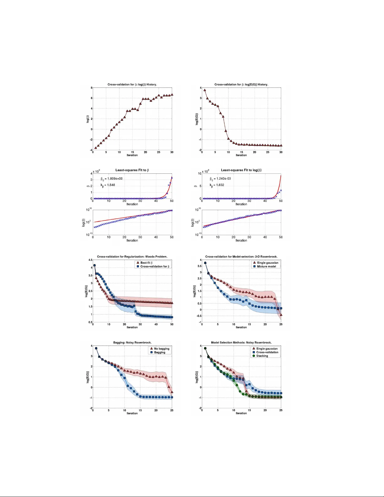
Bias-V ariance T rade-offs: No v el Applications Dev Ra jnara yan Da vid W olp ert No vem ber 18, 2021 Synon yms Bias-v ariance trade-offs, bias plus v ariance. Definition Consider a giv en random v ariable F and a random v ariable that we can modify , ˆ F . W e wish to use a sample of ˆ F as an estimate of a sample of F . The mean squared error betw een suc h a pair of samples is a sum of four terms. The first term reflects the statistical coupling b etw een F and ˆ F and is conv entionally ignored in bias-v ariance analysis. The second term reflects the inherent noise in F and is indep endent of the estimator ˆ F . Accordingly , w e c annot affect this term. In con trast, the third and fourth terms dep end on ˆ F . The third term, called the bias, is indep endent of the precise samples of b oth F and ˆ F , and reflects the difference b et ween the means of F and ˆ F . The fourth term, called the v ariance, is indep enden t of the precise sample of F , and reflects the inherent noise in the estimator as one samples it. These last tw o terms can b e mo dified by changing the choice of the estimator. In particular, on small sample sets, w e can often decrease our mean squared error b y , for instance, introducing a small bias that causes a large reduction the v ariance. While most commonly used in mac hine learning, this article shows that suc h bias-v ariance trade-offs are applicable in a m uch broader con text and in a v ariety of situations. W e also show, using exp eriments, ho w existing bias-v ariance trade-offs can b e applied in no vel circumstances to improv e the p erformance of a class of optimization algorithms. Motiv ation and Bac kground In its simplest form, the bias-v ariance decomp osition is based on the following idea. Sa y we hav e a Euclidean random v ariable F taking on v alues F distributed according to a densit y function p ( F ). W e w ant to estimate what v alue we w ould get if w ere to sample p ( F ). Ho wev er w e do not (or cannot) do this simply b y sampling F directly . Instead, to form our estimate, w e sample a differen t Euclidean random v ariable ˆ F taking on v alues ˆ F distributed according to p ( ˆ F ). Assuming a quadratic loss function, the qualit y of our estimate is measured by its Mean Squared Error (MSE): MSE( ˆ F ) ≡ Z p ( ˆ F , F ) ( ˆ F − F ) 2 d ˆ F dF . (1) Example 1: T o illustrate Eq. 1, consider the simplest t yp e of sup ervised machine learning problem, where there is a finite input space X , the output space Y is real num b ers, and there is no noise. In suc h learning there is some deterministic ‘target function’ f that maps eac h elemen t of X to a single elemen t of Y . There is a ‘prior’ probabilit y density function π ( f ) ov er target functions, and it gets sampled to pro duce some particular target function, f . Next, f is I ID sampled at a set of m inputs to produce a ‘training set’ D of input-output pairs. 1 F or simplicity , say there is some single fixed “prediction p oin t” x ∈ X . Our goal in sup ervised learning is to estimate f ( x ). How ev er f is not known to us. Accordingly , to p erform the estimation the training set is presen ted to a ‘learning algorithm’, which in resp onse to the training set pro duces a guess g ( x ) for the v alue f ( x ). This en tire sto chastic pro cedure defines a join t distribution π ( f , D , f ( x ) , g ( x )). W e can marginalize it to get a distribution π ( f ( x ) , g ( x )). Since g ( x ) is supp osed to b e an estimate of f ( x ), we can iden tify g ( x ) as the v alue ˆ F of the random v ariable ˆ F and f ( x ) as the v alue F of F . In other w ords, we can define p ( F , ˆ F ) = π ( f ( x ) , g ( x )). If we no w ask what the mean squared error is of the guess made by our learning algorithm for the v alue f ( x ), w e get Eq. 1. Note that one would exp ect that this F and ˆ F are statistically dep endent (Indeed, if they w eren’t dep enden t, then the dep endence of thelearning algorithm on D w ould b e p ointless.) F ormally , the dep endence can b e established b y writing p ( f ( x ) , g ( x )) = Z d D p ( f ( x ) , g ( x ) | D ) p ( D ) = Z d D p ( g ( x ) | f ( x ) , D ) p ( f ( x ) | D ) p ( D ) = Z d D p ( g ( x ) | D ) p ( f ( x ) | D ) p ( D ) (since the guess of the learning algorithm is determined in full by the training set), and then noting that in general this in tegral differs from the product p ( f ( x )) p ( g ( x )) =  Z d D p ( f ( x ) | D ) p ( D )   Z d D p ( g ( x ) | D ) p ( D )  . In Ex. 1 F and ˆ F are statistically coupled. Such coupling is extremely common. In practice though, suc h coupling is simply ignored in analyses of bias plus v ariance, without an y justification. In particular Ba yesian supervised learning av oids an y explicit consideration of bias plus v ariance. F or its part, non- Ba yesian sup ervised learning av oids consideration of the coupling by replacing the distribution p ( F, ˆ F ) with the asso ciated product of marginals, p ( F ) p ( ˆ F ). F or now we follow that latter practice. So our equation for MSE reduces to MSE( ˆ F ) = Z p ( ˆ F ) p ( F ) ( ˆ F − F ) 2 d ˆ F dF . (2) (If w e were to account for the coupling of ˆ F and ˆ F an additive correction term would need to b e added to the right-hand side. F or instance, see W olp ert [1997].) Using simple algebra, the righ t hand side of Eq. 2 can be written as the sum of three terms. The first is the v ariance of F . Since this is b eyond our con trol in designing the estimator ˆ F , we ignore it for the rest of this article. The second term inv olv es a mean that describ es the deterministic comp onen t of the error. This term dep ends on b oth the distribution of F and that of ˆ F , and quantifies ho w close the means of those distributions are. The third term is a v ariance that describ es sto c hastic v ariations from one sample to the next. This term is indep enden t of the random v ariable b eing estimated. F ormally , up 2 to an ov erall additive constant, we can write MSE( ˆ F ) = Z p ( ˆ F )( ˆ F 2 − 2 F ˆ F + F 2 ) d ˆ F , = Z p ( ˆ F ) ˆ F 2 d ˆ F − 2 F Z p ( ˆ F ) ˆ F d ˆ F + F 2 , = z }| { V ( ˆ F ) + [ E ( ˆ F )] 2 − 2 F E ( ˆ F ) + F 2 , = V ( ˆ F ) + [ F − E ( ˆ F )] 2 | {z } , = v ariance + bias 2 . (3) In light of Eq. 3, one wa y to try to reduce afexp ected quadratic e rror is to mo dify an estimator to trade-off bias and v ariance. Some of the most famous applications of such bias-v ariance trade-offs o ccur in parametric machine learning, where man y techniques hav e b een developed to exploit the trade-off. Ho wev er there are some extensions of that trade-off that could be applied in parametric mac hine learning that hav e b een ignored b y the comm unity . W e illustrate one of them here. Moreo ver, the bias-v ariance trade-off arises in many other fields b esides parameteric machine learn- ing. In particular, as we illustrate here, it arises in integral estimation and optimization. In the rest of this pap er we present some no vel applications of the bias-v ariance trade-off, and describ e some in- teresting features in eac h case. A recurring theme is that whenever a bias-v ariance trade-off arises in a particular field, w e can use man y techniques from parametric mac hine learning that ha v e b een dev elop ed for exploiting this trade-off. The nov el applications of the tradeoff discussed here are instances of the Probabilit y Collectiv es (PC) W olp ert and Ra jnara yan [2007], W olp ert et al. [2006], W olp ert and Bieni- a wski [2004a,b], Macready and W olp ert [2005], a general approach to using probability distributions to do blackbox optimization. Applications In this section, w e describ e some applications of the bias-v ariance tradeoff. First, we describ e Monte Carlo (MC) tec hniques for the estimation of integrals, and pro vide a brief analysis of bias-v ariance trade- offs in this context. Next, w e introduce the field of Monte Carlo Optimization (MCO), and illustrate that there are more subtleties inv olv ed than in simple MC. Then, w e describ e the field of Parametric Mac hine Learning, whic h, as will show, is formally iden tical to MCO. Finally , we present an application of P arametric Learning (PL) tec hniques to impro ve the p erformance of MCO algorithms. W e do this in the context of an MCO problem that is central to how PC addresses black-box optimization. Mon te Carlo Estimation of In tegrals Using Imp ortance Sampling Mon te Carlo metho ds are often the method of choice for estimating difficult high-dimensional integrals. Consider a function f : X → R , whic h we wan t to integrate ov er some region X ⊆ X , yielding the v alue F , as given by F = Z X dx f ( x ) . W e can view this as a random v ariable F , with density function given by a Dirac delta function centered on F . Therefore, the v ariance of F is 0, and Eq. 3 is exact. A p opular MC metho d to estimate this in tegral is imp ortance sampling [see Rob ert and Casella, 2004]. This exploits the la w of large num b ers as follows: i.i.d. samples x ( i ) , i = 1 , . . . , m are generated from a so-called importance distribution h ( x ) that w e con trol, and the associated v alues of the in tegrand, f ( x ( i ) ) are computed. Denote these ‘data’ by D = { ( x ( i ) , f ( x ( i ) ) , i = 1 , . . . , m } . (4) 3 No w, F = Z X dx h ( x ) f ( x ) h ( x ) , = lim m →∞ 1 m m X i =1 f ( x ( i ) ) h ( x ( i ) ) with probability 1. Denote by ˆ F the random v ariable with v alue given b y the sample av erage for D : ˆ F = 1 m m X i =1 f ( x ( i ) ) h ( x ( i ) ) . W e use ˆ F as our statistical estimator for F , as we broadly describ ed in the introductory section. Assum- ing a quadratic loss function, L ( ˆ F , F ) = ( F − ˆ F ) 2 , the bias-v ariance decomp osition describ ed in Eq. 3 applies exactly . It can b e sho wn that the estimator ˆ F is unbiased, that is, E ( ˆ F ) = F , where the mean is o ver samples of h . Consequently , the MSE of this estimator is just its v ariance. The c hoice of sampling distribution h that minimizes this v ariance is giv en b y [see Rob ert and Casella, 2004] h ? ( x ) = | f ( x ) | R X | f ( x 0 ) | dx 0 . By itself, this result is not very helpful, since the equation for the optimal imp ortance distribution con tains a similar in tegral to the one w e are trying to estimate. F or non-negative integrands f ( x ), the VEGAS algorithm [Lepage, 1978] describ es an adaptive metho d to find successiv ely b etter imp ortance distributions, by iteratively estimating F , and then using that estimate to generate the next imp ortance distribution h . In the case of these unbiased estimators, there is no trade-off b et ween bias and v ariance, and minimizing MSE is achiev ed by minimizing v ariance. Mon te Carlo Optimization Instead of a fixe d integral to ev aluate, consider a parametrized integral F ( θ ) = Z X dx f θ ( x ) . F urther, supp ose we are interested in finding the v alue of the parameter θ ∈ Θ that minimizes F ( θ ): θ ? = arg min θ ∈ Θ F ( θ ) . In the case where the functional form of f θ is not explicitly known, one approach to solv e this problem is a tec hnique called Mon te Carlo Optimization (MCO) [see Ermoliev and Norkin, 1998], in volving rep eated MC estimation of the integral in question with adaptive mo dification of the parameter θ . W e proceed by analogy to the case with MC. First, we in tro duce the θ -indexed random v ariable F ( θ ), all of whose components hav e delta-function distributions about the associated v alues F ( θ ). Next, we in tro duce a θ -indexed vector random v ariable ˆ F with v alues ˆ F ≡ { ˆ F ( θ ) ∀ θ ∈ Θ } . (5) Eac h real-v alued component ˆ F ( θ ) can b e sampled and viewed as an estimate of F ( θ ). F or example, let D b e a data set as describ ed in Eq. 4. Then for every θ , an y sample of D pro vides an asso ciated estimate ˆ F ( θ ) = 1 m m X i =1 f θ ( x ( i ) ) h ( x ( i ) ) . 4 That av erage serves as an estimate of F ( θ ). F ormally , ˆ F is a function of the random v ariable D , and is giv en by suc h av eraging ov er the elements of D . So, a sample of D pro vides a sample of ˆ F . A priori , w e make no restrictions on ˆ F , and so, in general, its comp onents may b e statistically coupled with one another. Note that this coupling arises ev en though we are, for simplicity , treating each function F ( θ ) as having a delta-function distribution, rather than as having a non-zero v ariance that w ould reflect our lac k of knowledge of the f ( θ ) functions. Ho wev er ˆ F is defined, given a sample of ˆ F , one wa y to estimate θ ? is ˆ θ ? = arg min θ ∈ Θ ˆ F ( θ ) W e call this approac h ‘natural’ MCO. As an example, say that D is a set of m samples of h , and let ˆ F ( θ ) , 1 m m X i =1 f θ ( x ( i ) ) h ( x ( i ) ) , as ab ov e. Under this choice for ˆ F , ˆ θ ? = arg min θ ∈ Θ 1 m m X i =1 f θ ( x ( i ) ) h ( x ( i ) ) . (6) W e call this approac h ‘naiv e’ MCO. Consider any algorithm that estimates θ ? as a single-v alued function of ˆ F . The estimate of θ ? pro duced by that algorithm is itself a random v ariable, since it is a function of the random v ariable ˆ F . Call this random v ariable ˆ θ ? , taking on v alues ˆ θ ? . Any MCO algorithm is defined by ˆ θ ? ; that random v ariable encapsulates the output estimate made by the algorithm. T o analyze the error of such an algorithm, consider the asso ciated random v ariable given by the true parametrized integral F ( ˆ θ ? ). The difference b etw een a sample of F ( ˆ θ ? ) and the true minimal v alue of the integral, F ( θ ? ) = min θ F ( θ ), is the error introduced b y our estimating that optimal θ as a sample of ˆ θ ? . Since our aim in MCO is to minimize F ( θ ), w e adopt the loss function L ( ˆ θ ? , θ ? ) , F ( ˆ θ ? ) − F ( θ ? ). This is in contrast to our discussion on MC integration, which inv olved quadratic loss. The curren t loss function just equals F ( ˆ θ ? ) up to an additive constan t F ( θ ? ) that is fixed by the MCO problem at hand and is b eyond our control. Up to that additive constant, the asso ciated exp ected loss is E ( L ) = Z d ˆ θ ? p ( ˆ θ ? ) F ( ˆ θ ? ) . (7) No w change co ordinates in this integral from the v alues of the scalar random v ariable ˆ θ ? to the v alues of the underlying v ector random v ariable ˆ F . The exp ected loss now b ecomes E ( L ) = Z d ˆ F p ( ˆ F ) F ( ˆ θ ? ( ˆ F )) . The natural MCO algorithm provides some insight into these results. F or that algorithm, E ( L ) = Z d ˆ F p ( ˆ F ) F (arg min θ ˆ F ( θ )) = Z d ˆ F ( θ 1 ) d ˆ F ( θ 2 ) . . . p ( ˆ F ( θ 1 ) , ˆ F ( θ 2 ) , . . . ) F (arg min θ ˆ F ( θ )) . (8) F or any fixed θ , there is an error betw een samples of ˆ F ( θ ) and the true v alue F ( θ ). Bias-v ariance considerations apply to this error, exacty as in the discussion of MC ab ov e. W e are not, how ev er, concerned with ˆ F for a single comp onent θ , but rather for a set Θ of θ ’s. 5 The simplest such case is where the comp onen ts of ˆ F (Θ) are indep endent. Ev en so, arg min θ ˆ F ( θ ) is distributed according to the laws for extrema of m ultiple indep endent random v ariables, and this distribution dep ends on higher-order moments of each random v ariable ˆ F ( θ ). This means that E [ L ] also dep ends on such higher-order moments. Only the first tw o moments, how ev er, arise in the bias and v ariance for any single θ . Thus, even in the simplest possible case, the bias-v ariance considerations for the individual θ do not provide a complete analysis. In most cases, the comp onents of ˆ F are not indep enden t. Therefore, in order to analyze E [ L ], in addition to higher moments of the distribution for eac h θ , w e must now also consider higher-order momen ts coupling the estimates ˆ F ( θ ) for different θ . Due to these effects, it ma y b e quite acceptable for all the comp onents ˆ F ( θ ) to hav e b oth a large bias and a large v ariance, as long as they still order the θ ’s correctly with res pect to the true F ( θ ). In such a situation, large co v ariances could ensure that if some ˆ F ( θ ) were incorrectly large, then ˆ F ( θ 0 ) , θ 0 6 = θ w ould also b e incorrectly large. This coupling b etw een the comp onents of ˆ F w ould preserve the ordering of θ ’s under F . So, ev en with large bias and v ariance for each θ , the estimator as a whole would still w ork w ell. Nev ertheless, it is sufficient to design estimators ˆ F ( θ ) with sufficiently small bias plus v ariance for each single θ . More precisely , supp ose that those terms are v ery small on the scale of differences F ( θ ) − F ( θ 0 ) for an y θ and θ 0 . Then by Chebyc hev’s inequality , w e know that the density functions of the random v ariables ˆ F ( θ ) and ˆ F ( θ 0 ) ha ve almost no o verlap. Accordingly , the probabilit y that a sample of ˆ F ( θ ) − ˆ F ( θ 0 ) has the opp osite sign of F ( θ ) − F ( θ 0 ) is almost zero. Eviden tly , E [ L ] is generally determined by a complicated relationship in volving bias, v ariance, co- v ariance, and higher moments. Natural MCO in general, and naive MCO in particular, ignore all of these effects, and consequen tly , often p erform quite p o orly in practice. In the next section w e discuss some wa ys of addressing this problem. P arametric Mac hine Learning There are man y versions of the basic MCO problem describ ed in the previous section. Some of the b est-explored arise in parametric densit y estimation and parametric sup ervised learning, whic h together comprise the field of Parametric mac hine Learning (PL). In particular, parametric sup ervised learning attempts to solve arg min θ ∈ Θ Z dx p ( x ) Z dy p ( y | x ) f θ ( x ) . Here, the v alues x represent inputs, and the v alues y represent corresp onding outputs, generated ac- cording to some sto chastic pro cess defined b y a set of conditional distributions { p ( y | x ) , x ∈ X } . T ypically , one tries to solv e this problem by casting it as an MCO problem, F or instance, say we adopt a quadratic loss betw een a predictor z θ ( x ) and the true v alue of y . Using MCO notation, we can express the asso ciated sup ervised learning problem as finding arg min θ F ( θ ), where l θ ( x ) = Z dy p ( y | x ) ( z θ ( x ) − y ) 2 , f θ ( x ) = p ( x ) l θ ( x ) , F ( θ ) = Z dx f θ ( x ) . (9) Next, the argmin is estimated by minimizing a sample-based estimate of the F ( θ )’s. More precisely , w e are giv en a ‘training set’ of samples of p ( y | x ) p ( x ), { ( x ( i ) , y i ) i = 1 , . . . , m } . This training set pro vides a set of asso ciated estimates of F ( θ ): ˆ F ( θ ) = 1 m m X i =1 l θ ( x ( i ) ) . 6 These are used to estimate arg min θ F ( θ ), exactly as in MCO. In particular, one could estimate the minimizer of F ( θ ) by finding the minimium of ˆ F ( θ ), just as in natural MCO. As mentioned ab o ve, this MCO algorithm can p erform very p o orly in practice. In PL, this p o or performance is called ‘ov erfitting the data’. There are several formal approaches that hav e been explored in PL to try to address this ‘o verfitting the data’. In terestingly , none are based on direct consideration of the random v ariable F ( ˆ θ ? ( ˆ F )) and the ramifications of its distribution for exp ected loss (cf. Eq. 8). In particular, no work has applied the mathematics of extrema of m ultiple random v ariables to analyze the bias-v ariance-cov ariance trade-offs encapsulated in Eq. 8. The PL approac h that p erhaps comes closest to such direct consideration of the distribution of F ( ˆ θ ? ) is uniform conv ergence theory , which is a cen tral part of Computational Learning Theory [see Angluin, 1992]. Uniform con vergence theory starts by crudely encapsulating the quadratic loss formula for exp ected loss under natural MCO, Eq. 8. It do es this by considering the worst-case b ound, o ver p ossible p ( x ) and p ( y | x ), of the probability that F ( θ ? ) exceeds min θ F ( θ ) by more than κ . It then examines how that b ound v aries with κ . In particular, it relates such v ariation to characteristics of the set of functions { f θ : θ ∈ Θ } , e.g., the ‘VC dimension’ of that set [see V apnik, 1982, 1995]. Another, historically earlier approach, is to apply bias-plus-v ariance considerations to the entire PL algorithm ˆ θ ? , rather than to eac h ˆ F ( θ ) separately . This approac h is applicable for algorithms that do not use natural MCO, and even for non-parametric supervised learning. As formulated for parameteric sup ervised learning, this approac h combines the formulas in Eq. 9 to write F ( θ ) = Z dxdy p ( x ) p ( y | x )( z θ ( x ) − y ) 2 . This is then substituted into Eq. 7, giving E [ L ] = Z d ˆ θ ? dx dy p ( x ) p ( y | x ) p ( ˆ θ ? )( z ˆ θ ? ( x ) − y ) 2 = Z dx p ( x )  Z d ˆ θ ? dy p ( x ) p ( y | x ) p ( ˆ θ ? )( z ˆ θ ? ( x ) − y ) 2  . (10) The term in square brac kets is an x -parameterized exp ected quadratic loss, which can b e decomp osed in to a bias, v ariance, etc., in the usual w ay . This form ulation eliminates an y direct concern for issues lik e the distribution of extrema of multiple random v ariables, co v ariances betw een ˆ F ( θ ) and ˆ F ( θ 0 ) for differen t v alues of θ , and so on. There are n umerous other approac hes for addressing the problems of natural MCO that hav e b een explored in PL. P articulary imp ortan t among these are Ba y esian approaches, e.g., Buntine and W eigend [1991], Berger [1985], Mack ay [2003]. Based on these approaches, as well as on intuition, many p ow erful tec hniques for addressing data-ov erfitting ha ve b een explored in PL, including regularization, cross- v alidation, stacking, bagging, etc. Essen tially all of these tec hniques can b e applied to any MCO problem, not just PL problems. Since many of these tec hniques can b e justified using Eq. 10, they pro vide a wa y to exploit the bias-v ariance trade-off in other domains b esides PL. PLMCO In this section, we illustrate how PL techniques that exploit the bias-v ariance decomp osition of Eq. 10 can b e used to improv e an MCO algorithm used in a domain outside of PL. This MCO algorithm is a v ersion of adaptive imp ortance sampling, somewhat similar to the CE metho d [Rubinstein and Kro ese, 2004], and is related to function smo othing on contin uous spaces. The PL tec hniques describ ed are applicable to any other MCO problem, and this particular one is chosen just as an example. 7 MCO Problem Description Consider the problem of finding the θ -parameterized distribution q θ that minimizes the asso ciated ex- p ected v alue of a function G : R n → R , i.e., find arg min θ E q θ [ G ] . W e are interested in versions of this problem where we do not know the functional form of G , but can obtain its v alue G ( x ) at any x ∈ X . Similarly w e cannot assume that G is smo oth, nor can we ev aluate its deriv ativ es directly . This scenario arises in man y fields, including blackbox optimization [see W olp ert et al., 2006], and risk minimization [see Ermoliev and Norkin, 1998]. W e b egin by expressing this minimization problem as an MCO problem. W rite E q θ [ G ] = Z X dx q θ ( x ) G ( x ) Using MCO terminology , f θ ( x ) = q θ ( x ) G ( x ) and F ( θ ) = E q θ [ G ]. T o apply MCO, we m ust define a v ector-v alued random v ariable ˆ F with comp onents indexed by θ , and then use a sample of ˆ F to estimate arg min θ E q θ [ G ]. In particular, to apply naive MCO to estimate arg min θ E q θ ( G ), w e first i.i.d. sample a densit y function h ( x ). By ev aluating the asso ciated v alues of G ( x ) we get a data set D ≡ ( D X , D G ) = ( { x ( i ) : i = 1 , . . . , m } , { G ( x ( i ) ) : i = 1 , . . . , m } ) . The asso ciated estimates of F ( θ ) for each θ are ˆ F ( θ ) , 1 m m X i =1 q θ ( x ( i ) ) G ( x ( i ) ) h ( x ( i ) ) . (11) The asso ciated naive MCO estimate of arg min θ E q θ [ G ] is ˆ θ ? ≡ arg min θ ˆ F ( θ ) . Supp ose Θ includes all p ossible densit y functions o ver x ’s. Then the q θ minimizing our estimate is a delta function ab out the x ( i ) ∈ D X with the low est asso ciated v alue of G ( x ( i ) ) /h ( x ( i ) ). This is clearly a p oor estimate in general; it suffers from ‘data-o verfitting’. Pro ceeding as in PL, one wa y to address this data-o verfitting is to use regularization. In particular, we can use the entropic regularizer, giv en b y the negativ e of the Shannon en tropy S ( q θ ). So we now wan t to find the minimizer of E q θ [ G ( x )] − T S ( q θ ), where T is the regularization parameter. Equiv alently , we can minimize β E q θ [ G ( x )] − S ( q θ ), where β = 1 /T . This changes the definition of ˆ F from the function given in Eq. 11 to ˆ F ( θ ) , 1 m m X i =1 β q θ ( x ( i ) ) G ( x ( i ) ) h ( x ( i ) ) − S ( q θ ) . Find the solution to this minimization problem is the fo cus of the PC approach to blackbox optimization. Solution Methodology Unfortunately , it can b e difficult to find the θ globally minimizing this new ˆ F for an arbitrary D . An alternativ e is to find a close approximation to that optimal θ . One w ay to do this is as follo ws. First, w e find the minimizer of 1 m m X i =1 β p ( x ( i ) ) G ( x ( i ) ) h ( x ( i ) ) − S ( p ) (12) 8 o ver the set of al l p ossible distributions p ( x ) with domain X . W e then find the q θ that has minimal Kullbac k-Leibler (KL) div ergence from this p , ev aluated ov er D X . That serv es as our approximation to arg min θ ˆ F ( θ ), and therefore as our estimate of the θ that minimizes E q θ ( G ). The minimizer p of Eq. 12 can b e found in closed form; ov er D X it is the Boltzmann distribution p β ( x ( i ) ) ∝ exp( − β G ( x ( i ) )) . The KL div ergence in D X from this Boltzmann distribution to q θ is F ( θ ) = KL( p β k q θ ) = Z X dx p β ( x ) log  p β ( x ) q θ ( x )  . The minimizer of this KL divergence is given b y θ † = arg min θ [ − m X i =1 exp( − β G ( x ( i ) )) h ( x ( i ) ) log( q θ ( x ( i ) ))] . (13) θ † is an appro ximation to the estimate of the θ that minimizes E q θ ( G ) given by the regularized version of naiv e MCO. Our incorp oration of regularization here has the same motiv ation as it do es in PL: to reduce bias plus v ariance. Log-conca ve Densities If q θ is log-conca ve in its parameters θ , then the minimization problem in Eq. 13 is a con v ex optimization problem, and the optimal parameters can b e found closed-form. Denote the likelihoo d ratios by s ( i ) = exp( − β G ( x ( i ) )) /h ( x ( i ) ). Differen tiating Eq. 13 with resp ect to the parameters µ and Σ − 1 and setting them to zero yields µ ? = P D s ( i ) x ( i ) P D s ( i ) Σ ? = P D s ( i ) ( x ( i ) − µ ? )( x ( i ) − µ ? ) T P D s ( i ) Mixture Models The single Gaussian is a fairly restrictive class of mo dels. Mixture mo dels can significantly improv e flexibilit y , but at the cost of conv exity of the KL distance minimization problem. Ho wev er, a plethora of tec hniques from supervized learning, in particular the Exp ectation Maximization (EM) algorithm, can b e applied with minor mo difications. Supp ose q θ is a mixture of M Gaussians, that is, θ = ( µ, Σ , φ ) where φ is the mixing p.m.f, w e can view the problem as one where a hidden v ariable z decides which mixture comp onent eac h sample is dra wn from. W e then hav e the optimization problem minimize − X D p ( x ( i ) ) h ( x ( i ) ) log  q θ ( x ( i ) , z ( i ) )  . F ollo wing the standard EM pro cedure, w e get the algorithm describ ed in Eq. 14. Since this is a noncon vex problem, one t ypically runs the algorithm m ultiple times with random initializations of the parameters. E-step: F or eac h i, set Q i ( z ( i ) ) = p ( z ( i ) | x ( i ) ) , that is, w ( i ) j = q µ, Σ ,φ ( z ( i ) = j | x ( i ) ) , j = 1 , . . . , M . M-step: Set µ j = P D w ( i ) j s ( i ) x ( i ) P D w ( i ) j s ( i ) , Σ j = P D w ( i ) j s ( i ) ( x ( i ) − µ j )( x ( i ) − µ j ) T P D w ( i ) j s ( i ) , φ j = P D w ( i ) j s ( i ) P D s ( i ) , (14) 9 T est Problems T o compare the p erformance of this algorithm with and without the use of PL techniques, w e use a couple of very simple academic problems in tw o and four dimensions - the Rosen bro ck function in t wo dimensions, given b y G R ( x ) = 100( x 2 − x 2 1 ) 2 + (1 − x 1 ) 2 , and the W o o ds function in four dimensions, given by giv en b y G woods ( x ) = 100( x 2 − x 1 ) 2 + (1 − x 1 ) 2 + 90( x 4 − x 2 3 ) 2 + (1 − x 3 ) 2 +10 . 1[(1 − x 2 ) 2 + (1 − x 4 ) 2 ] + 19 . 8(1 − x 2 )(1 − x 4 ) . F or the Rosenbrock, the optimum v alue of 0 is achiev ed at x = (1 , 1), and for the W o o ds problem, the optim um v alue of 0 is ac hieved at x = (1 , 1 , 1 , 1). Application of PL T ec hniques As mentioned ab ov e, there are many PL tec hniques beyond regularization that are designed to optimize the trade-off b etw een bias and v ariance. So having cast the solution of arg min q θ E ( G ) as an MCO problem, we can apply those other PL tec hniques instead of (or in addition to) entropic regularization. This should improv e the performance of our MCO algorithm, for the exact same reason that using those tec hniques to trade off bias and v ariance improv es p erformance in PL. W e briefly men tion some of those alternativ e tec hniques here. The ov erall MCO algorithm is broadly describ ed in Alg. 1. F or the W o o ds problem, 20 samples of x are drawn from the up dated q θ at each iteration, and for the Rosenbrock, 10 samples. F or comparing v arious metho ds and plotting purp oses, 1000 samples of G ( x ) are drawn to ev aluate E q θ [ G ( x )]. Note: in an actual optimization, we will not b e drawing these test samples! All the p erformance results in Fig. 1 are based on 50 runs of the PC algorithm, randomly initialized eac h time. The sample mean p erformance across these runs is plotted along with 95% confidence interv als for this sample mean (shaded regions). Algorithm 1 Ov erview of pq minimization using Gaussian mixtures 1: Draw uniform random samples on X 2: Initialize regularization parameter β 3: Compute G ( x ) v alues for those samples 4: rep eat 5: Find a mixture distribution q θ to minimize sampled pq KL distance 6: Sample from q θ 7: Compute G ( x ) for those samples 8: Up date β 9: until T ermination 10: Sample final q θ to get solution(s). Cross-v alidation for Regularization: W e note that we are using regularization to reduce v ariance, but that regularization introduces bias. As is done in PL, we use standard k -fold cross-v alidation to tradeoff this bias and v ariance. W e do this b y partitioning the data in to k disjoin t sets. The held-out data for the i th fold is just the i th partition, and the held-in data is the union of all other partitions. First, we ‘train’ the regularized algorithm on the held-in data D t to get an optimal set of parameters θ ? , then ‘test’ this θ ? b y considering unregularized p erformance on the held-out data D v . In our context, ‘training’ refers to finding optimal parameters by KL distance minimization using the held-in data, and ‘testing’ refers to estimating E q θ [ G ( x )] on the held-out data using the follo wing formula [Rob ert and 10 Casella, 2004]. b g ( θ ) = X D v q θ ( x ( i ) ) G ( x ( i ) ) h ( x ( i ) ) X D v q θ ( x ( i ) ) h ( x ( i ) ) . W e do this for several v alues of the regularization parameter β in the interv al k 1 β < β < k 2 β , and c ho ose the one that yield the best held-out performance, a veraged o ver all folds. F or our experiments, k 1 = 0 . 5 , k 2 = 3, and we use 5 equally-spaced v alues in this in terv al. Having found the b est regularization parameter in this range, we then use al l the data to minimize KL distance using this optimal v alue of β . Note that all cross-v alidation is done without an y additional ev aluations of G ( x ). Cross-v alidation for β in PC is similar to optimizing the annealing schedule in sim ulated annealing. This ‘auto-annealing’ is seen in Fig. 1.a, which shows the v ariation of β with iterations of the Rosenbrock problem. It can b e seen that β v alue sometimes decreases from one iteration to the next. This can never happen in an y kind of ‘geometric annealing sc hedule’, β ← k β β , k β > 1, of the sort that is often used in most algorithms in the literature. In fact, we ran 50 trials of this algorithm on the Rosenbrock and then computed a b est-fit geometric v ariation for β , that is, a nonlinear least squares fit to v ariation of β , and a linear least squares fit to the v ariation of log( β ). These are shown in Figs. 1.c. and 1.d. As can b e seen, neither is a v ery go o d fit. W e then ran 50 trials of the algorithm with the fixed up date rule obtained by b est-fit to log( β ), and found that the adaptive setting of β using cross-v alidation p erformed an order of magnitude b etter, as shown in Fig. 1.e. Cross-v alidation for Mo del Selection: Given a set Θ (sometimes called a mo del class) to choose θ from, w e can find an optimal θ ∈ Θ. But ho w do w e choose the set Θ? In PL, this is done using cross-v alidation. W e choose that set Θ such that arg min θ ∈ Θ ˆ F ( θ ) has the best held-out p erformance. As b efore, we use that mo del class Θ that yields the lo west estimate of E q θ [ G ( x )] on the held-out data. W e demonstrate the use of this PL technique for minimizing the Rosenbrock problem, which has a long curved v alley that is p o orly approximated by a single Gaussian. W e use cross-v alidation to choose b et ween a Gaussian mixture with up to 4 components. The improv emen t in p erformance is sho wn in Fig. 1.d. Bagging: In bagging Breiman [1996a], we generate multiple data sets b y resampling the given data set with replacemen t. These new data sets will, in general, contain replicates. W e ‘train’ the learning algorithm on each of these resampled data sets, and a verage the results. In our case, we av erage the q θ got by our KL div ergence minimization on each data set. PC works even on sto c hastic ob jective functions, and on the noisy Rosen bro ck, we implemented PC with bagging by resam pling 10 times, and obtained significant performance gains, as seen in Fig. 1.g. Stac king: In bagging, we com bine estimates of the same learning algorithm on different data sets generated by resampling, whereas in stacking Breiman [1996b], Smyth and W olp ert [1999], we com bine estimates of different learning algorithms on the same data set. These combined estimated are often b etter than any of the single estimates. In our case, we combine the q θ obtained from our KL divergence minimization algorithm using multiple models Θ. Again, Fig. 1.h shows that cross-v alidation for mo del selection p erforms better than a single mo del, and stacking p erforms slightly b etter than cross-v alidation. Conclusions The conv en tional goal of reducing bias plus v ariance has interesting applications in a v ariety of fields. In straigh tforward applications, the bias-v ariance trade-offs can decrease the MSE of estimators, reduce the generalization error of learning algorithms, and so on. In this article, w e describ ed a nov el application of bias-v ariance trade-offs: we placed bias-v ariance trade-offs in the context of Mon te Carlo Optimization, and discussed the need for higher momen ts in the trade-off, suc h as a bias-v ariance-co v ariance trade-off. W e also show ed a wa y of applying just a bias-v ariance trade-off, as used in P arametric Learning, to impro ve the p erformance of Mon te Carlo Optimization algorithms. 11 a. b. c. d. e. f. g. h. Figure 1: V arious PL T ec hniques Impro ve MCO p erformance. 12 References D. H. W olp ert. On bias plus v ariance. Neur al Computation , 9:1211–1244, 1997. D. H. W olp ert and D. Ra jnaray an. Parametric learning and monte carlo optimization. Av ailable at h ttp://arxiv.org/abs/0704.1274, 2007. D. H. W olp ert, C. E. M. Strauss, and D. Ra jnaray an. Adv ances in distributed optimization using probabilit y collectiv es. A dvanc es in Complex Systems , 9(4):383–436, 2006. D. H. W olpert and S. Bieniawski. Distributed control by lagrangian steep est descent. In Pr o c. of the IEEE Contr ol and De cision Conf. , pages 1562–1567, 2004a. D. H. W olp ert and S. Bieniawski. Adaptive distributed control: b eyond single-instant categorical v ari- ables. In A. Sko wron et al, editor, Pr o c e e dings of MSRAS04 . Springer V erlag, 2004b. William Macready and David H. W olp ert. Distributed constrained optimization with semico ordinate transformations. submitted to Journal of Op erations Research, 2005. C. P . Rob ert and G. Casella. Monte Carlo Statistic al Metho ds . Springer-V erlag, New Y ork, 2004. G. P . Lepage. A new algorithm for adaptive m ultidimensional integration. Journal of Computational Physics , 27:192–203, 1978. Y. M. Ermoliev and V. I. Norkin. Monte carlo optimization and path dep endent nonstationary laws of large n umbers. T ec hnical Rep ort IR-98-009, International Institute for Applied Systems Analysis, Marc h 1998. D. Angluin. Computational learning theory: Survey and selected bibliography . In Pr o c e e dings of the Twenty-F ourth Annual ACM Symp osium on The ory of Computing, May 1992 , 1992. V. N. V apnik. Estimation of Dep endenc es Base d on Empiric al Data . Springer, 1982. V. N. V apnik. The Natur e of Statistic al L e arning The ory . Springer, 1995. W. Buntine and A. W eigend. Bay esian back-propagation. Complex Systems , 5:603–643, 1991. J. M. Berger. Statistic al De cision the ory and Bayesian Analysis . Springer-V erlag, 1985. D. Mack ay . Information the ory, infer enc e, and le arning algorithms . Cam bridge Universit y Press, 2003. R. Rubinstein and D. Kro ese. The Cr oss-Entr opy Metho d . Springer, 2004. L. Breiman. Bagging predictors. Machine L e arning , 24(2):123–140, 1996a. L. Breiman. Stac ked regression. Machine L e arning , 24(1):49–64, 1996b. P . Sm yth and D. W olp ert. Linearly combining density estimators via stacking. Machine L e arning , 36 (1-2):59–83, 1999. 13