Analysis of the Karmarkar-Karp Differencing Algorithm

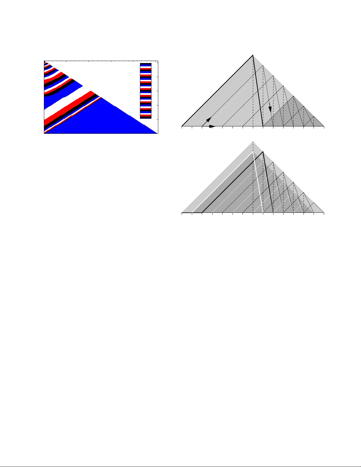
EPJ manuscript No. (will be inserted by the editor) Analysis of the Karmarkar -Karp Differencing Algorithm Stefan Boettcher 1 and Stephan Mertens 2 , 3 1 Department of Physics, Emory Uni versity , Atlanta GA 30322-243 0, U.S.A. 2 Institut f ¨ ur Theoretische Physik, Otto-von -Guericke Univ ersit ¨ at, PF 4120, 39016 Magdeb urg, Germany 3 Santa Fe Institute, 1399 Hyde Park Road , Santa Fe, New Mex ico 87501, U.S. A. October 27, 2018 Abstract The Karmarkar-Karp differen cing algorithm is t he best known polynomial time heuristic for t he number partitioning problem, fundamental in both theoretical computer science and statistical physics. W e analyze the per- formance of the diffe rencing algorithm on random instances by mapping it to a nonlinear rate equation. Our analysis rev eals strong finite size ef fects that explain why the precise asymptotics of the differencing solution is hard to establish by simulations. The asymptotic series emerging from the rate equation satisfies all kno wn bounds on the Karmarkar- Karp a lgorithm and p rojects a scaling n − c ln n , where c = 1 / ( 2 l n 2 ) = 0 . 7213 . . . . Our calculations re veal subtle relations between the algorithm and Fibonacci-like sequen ces, and we establish an e xplicit identity to that effect. P A CS. 02.60.Pn Numerical optimization – 89.75.Da Systems ob eying scaling laws – 89.75.Fb St ructures and orga- nization in comple x systems 1 Introduction Consider a list of n positi ve numbers. Replacing the two largest number s by their dif ference yields a ne w list of n − 1 numbers. Iterating this operation n − 1 times lea ves us with a single num- ber . Intuiti vely we expect this number to be much smaller than all the n umbers in the orig inal list. But ho w small? T his is the question that we address in the present paper . The operation that replaces two numbers in a list by their difference is called differ encing , and the proce dure that itera- ti vely selects the tw o lar gest numbers for dif feren cing is k nown as lar ges t differ encing method or LDM. This metho d was intro- duced in 19 82 b y Ka rmarkar and Karp [1] as an algorithm for solving the number partitioning problem ( N P P ) : Given a list a 1 , a 2 , . . . , a n of positive numbers, find a partition, i.e . a subset A ⊂ { 1 , . . . , n } s uch that the discrepan cy D ( A ) =    ∑ i ∈ A a i − ∑ i 6∈ A a i    , (1) is minimized. Obviously , LDM amounts to deciding iterati vely that the two largest numbers will b e put on different sides of the partition , b ut to def er the decision on what side to pu t each number . The final num ber then represents the discrepancy . Despite its simple definition , the N P P is o f consid erable importan ce both in theoretical computer science an d statisti- cal physics. The N P P is NP-hard, which mean s (a) that no al- gorithm is known that is essentially faster than exhaustively searching through all 2 n partitions, and ( b) that th e N P P is com - putationally eq uiv alent to m any famous problems like th e Tra v- eling Salesman Problem or the Satisfiability Prob lem [2]. In fact, the N P P is o ne of Gar ey and John son’ s six basic NP-h ard problem s that lie at the heart of the theory of NP-completeness [3], and it is the only on e of these pr oblems that actually deals with n umbers. Hence it is o ften cho sen as a ba se for NP-h ard- ness proo fs o f other pr oblems in volving n umbers, like bin p ack- ing, m ultiprocessor scheduling [4], quad ratic prog ramming o r knapsack pr oblems. Th e N P P was also th e ba se of one of the first public key crypto systems [5]. In statistical p hysics, the significance of th e N P P results from the fact that it was the first system for which th e local REM scenario was established [6, 7]. The notion loc al REM scenario r efers to systems which loca lly (o n the energy scale) behaves like Der rida’ s random energy m odel [8, 9]. It is con- jectured to be a universal featur e of ran dom, discrete systems [10]. Recently , this conjecture has been proven for se veral spin glass models [11, 12] and for directed polymer s in random me- dia [13]. Considering the NP-hard ness of the prob lem it is no sur- prise that LDM (which runs in polynomial ti me) will generally not find the o ptimal so lution but an a pproxim ation. Our initial question ask s for the q uality o f the LDM solu tion to N P P , and to a ddress this qu estion we will f ocus on ran dom instances of the N P P wh ere the numbers a j are indepe ndent, identically dis- tributed ( i.i.d.) rando m numb ers, u niformly distributed in the unit interval. L et L n denote the outp ut o f L DM on such a list. Y akir [14] proved tha t th e expec tation E [ L n ] is asym ptotically bound ed by n − b ln n ≤ E [ L n ] ≤ n − a ln n , (2) where a and b are (unknown) constants such that b ≥ a ≥ 1 2 ln 2 = 0 . 721 3 . . . . (3) In this contribution we will argue that b = a = 1 2 ln 2 . 2 Stefan Boettcher, Stephan Mertens: Analysis of the Karmarkar-Karp Dif ferencing Algorithm The pap er is organized as follows. W e start with a comp re- hensive descriptio n of the differencing algorithm, a simple (b ut wrong) argumen t that yields th e scaling (2) a nd a presentation of simulation d ata th at seems to vio late the asymp totic bou nd (3). In section 3 we refo rmulate LDM in terms o f a stochastic recursion on parameters of exponential v ariates. This recursion will then be simplified to a deter ministic, n onlinear rate equ a- tion in section 4. A numerical investigation o f this rate equation reveals a s tructur e in the dynamics of LDM that can be used as an Ansatz to simplify both the exact recur sions and the r ate equation. Th is will lead to a simple, Fib onacci like recu rsion (section 5 ) and to an analytic solution of the rate equation (sec- tion 6) . In b oth cases we can derive the asymptotics includ ing the correction s to scaling, and we claim tha t a similar asymp- totic expansion holds for the o riginal LDM. The latter claim is corrob orated by fitting th e asymptotic expansion to the avail- able numerical data on LDM. 2 Differencing Algorithm (c) (d) (a) (b) 1 5 6 7 8 3 1 2 1 4 4 Figure 1. The dif ferencing algorithm in action. The d ifferencing scheme a s descr ibed in the introdu ction giv es th e value of the d iscrepancy , b ut not th e actu al p artition. For that we need some addition al bookkeep ing, which is most easily implem ented in terms of gr aphs ( Fig. 1 ). The algo rithm maintains a list of roo ted trees where ea ch ro ot is labeled with a numb er . The algorith m starts with n tre es of size o ne and the roots labeled with the numbers a i . Then the follo wing steps are iterated until a single rooted tree of size n remains: 1. Among all roo ts, find those with th e largest ( x ) and second largest ( y ) label. 2. Join nodes x and y with an edge, declar e node x as the r oot of the new tree and relabel it with x − y . After n − 1 iteratio ns all nodes are spa nned by a tree w hose root is lab eled by the final discrep ancy . This tree can easily be two-colored, and the colors represent the desired partition. Fig. 1 illustrates this p rocedur e on the instance ( 4 , 5 , 6 , 7 , 8 ) . The final tw o colorin g co rrespond s to the partition ( 4 , 5 , 7 ) ver- sus ( 6 , 8 ) with discrepan cy 2. Note that the optim um p artition ( 4 , 5 , 6 ) versus ( 7 , 8 ) ac hiev es discrepancy 0. T echn ically , L DM boils d own to d eleting items fro m and inserting items into a sorted list of size n . This can be done in time O ( n ln n ) using an advanced data stru cture like a h eap [15]. Henc e LDM is very efficient, but how goo d is it? As we have alread y seen in the example, LDM can miss th e op- timal partition. And for rand om instance s, th e cor ridor ( 2) is far above the tru e optimu m, which is known to scale like Θ ( √ n 2 − n ) [7]. Y et LDM yield s the best r esults th at can be ach iev ed in polyno mial time. Many alternative algor ithms have b een in ves- tigated in the past [16, 17], but th ey all pr oduce results worse than (2). The fe w algorithms th at can ac tually compete with the Karmarkar-Karp procedu re use the same elementary differenc- ing ope ration [1 8, 19]. It seems as if the differencing scheme marks an inherent barrier for polyno mial time algorithms. The following argumen t explains th e scaling ( 2). The typ- ical distance between ad jacent p airs of the n num bers in th e interval [ 0 , 1 ] is n − 1 . Hen ce after n / 2 d ifferencing oper ations we are left with n / 2 numb ers in the in terval [ 0 , n − 1 ] . Th e typi- cal distance between pairs is now 2 n − 2 . After another round of n / 4 d ifferencing operation s we get n / 4 nu mbers in the r ange [ 0 , 8 n − 3 ] . I n gener al, after 2 k differencing operation s we are left with n / 2 k number s in the r ange [ 0 , 2 ( k 2 ) n − k ] . Reducin g the original list to a single numbe r requires k = lo g 2 n differencing operation s, and applying the above argument all the w ay down suggests that E [ L n ] ∝ n − c ln n (4) with c = 1 2 ln 2 = 0 . 721 . . . . (5) As we w ill see, this is the right scaling , y et the argument ca n- not be correc t. This follows from the fact th at it predicts the same scalin g for the pair ed differencing metho d (PDM). Here in each r ound all pair s of adjacen t number s are replaced by their difference in parallel. This method, howe ver , yields an av erage discrepancy of order Θ ( n − 1 ) [20]. Y et, our analysis belo w sug- gests that (4) an d (5) ind eed descr ibe the asympto tic behavior correctly , although a far more subtle treatment is required. An obviou s app roach to find th e quality o f LDM are sim- ulations. W e ran LDM on ran dom instances of varying size n , and Figu re 2 shows the r esults for E [ L n ] . Ap parently ln E [ L n ] scales like ln 2 n , in agree ment with ( 2) and (4). A linear fit seems to yield c ≃ 0 . 65 for the co nstant in (4), which clearly violates the boun d c ≥ 1 / 2 ln 2. App arently even n = 1 0 6 is to o small to see the tru e asymptotic behavior . This may be t he reason why Monte Carlo studies of LDM nev er ha ve been published. A plot of th e probability density function (pdf) of L n / E [ L n ] reveals a data collapse varying values of n (Fig. 3). Apparently the complete statistics of L n is asymptotically do minated by a single scale n − c ln n . Some technical notes ab out simulating LDM ar e app ro- priate. Differencin g means sub tracting nu mbers over a nd over again. Th e numerica l p recision must be adju sted car efully to Stefan Boettcher, Stephan Mertens: Analysis of the Karmarkar-Karp Dif ferencing Algorithm 3 50 100 150 ln 2 n 0 25 50 75 100 -ln E[ L n ] Figure 2. R esults of L DM applied to n random i.i. d. numbers, uni- formly drawn from the unit interval. Each data point represents be- tween 10 5 (large n ) and 10 7 samples (small n ). The solid line is the linear fit − ln E [ L n ] = 1 . 42 + 0 . 65 ln 2 n . 0 2 4 6 8 L n / E[L n ] 10 -3 10 -2 10 -1 10 0 n = 10 2 n = 10 3 n = 10 4 n = 10 5 Figure 3. Prob ability density function of L n / E [ L n ] . support this and to be able to repre sent the fina l d iscrepancy of order n − c ln n . W e used the freely av ailable GMP librar y [21 ] for the require d multiple precision arithmetic and ran all simu- lations on ℓ -bit integers wh ere th e numb er o f bits ran ges from ℓ = 40 (for n = 2 0) to ℓ = 30 0 for n = 1 . 5 · 1 0 7 . Th e integer discrepancies w ere th en re scaled by 2 − ℓ . The p seudo ran dom number generator was taken from the TRNG library [2 2]. 3 Exact Recursions A commo n problem in the average-case analysis of algo rithms like LDM is that num bers become conditioned and cease to be indepen dent as the algo rithm pro ceeds. Lueker [2 0] pro posed to use e xpon ential instead of uniform variates to cope with this problem . Let X 1 , . . . , X n + 1 be i.i.d . ran dom exponentials with mean 1 and consid er the par tial sums S k = ∑ k i = 1 X i . Th en the joint distrib ution of the ratios S k / S n + 1 , k = 1 , . . . , n , is the same as that o f the ord er statistics of n i.i.d . unifor m variates f rom [ 0 , 1 ] [2 3]. As a consequence, LDM will produce the same dis- tribution of d ata no matter whether it is run on unifor m v ariates or on S k / S n + 1 . Let ˆ L n denote the result of LDM on the par- tial sums S 1 , S 2 , . . . , S n . Since the output of LDM is linear in its input, we ha ve ˆ L n D = S n + 1 L n , (6) where S n + 1 is th e sum of n + 1 i.i.d. exponen tial variates an d the notatio n X D = Y indica tes that the rando m v ariable X an d Y have the same distribution. T he pro bability density of S n + 1 is the gamma density g n + 1 ( s ) = s n n ! e − s . (7) T aking expectations of both sides of (6) we get E [ L n ] = E  ˆ L n  n + 1 . (8) This allows us to derive the asympto tics of E [ L n ] fr om the asymptotics of E  ˆ L n  . Expon ential variates are well suited for the analysis of LDM because the sum and dif ference of two exponen tial variates are again expon ential variates. Once started o n expon ential vari- ates, LDM keeps working on expo nentials all th e tim e. This allows us to express the operation of LDM in ter ms of a re cur- si ve equatio n fo r th e param eters of exp onential densities [14]. W e start with the following Lemma: Lemma 1 Let X 1 and X 2 be in depende nt exponen tial random variables with pa rameter λ 1 and λ 2 , resp.. The pr obability of the event X 1 < X 2 is given by P ( X 1 < X 2 ) = λ 1 λ 1 + λ 2 . (9) Furthermore , co nditioned o n th e event X 1 < X 2 , the varia bles X 1 and X 2 − X 1 ar e indep endent exponentials with parameters λ 1 + λ 2 (for X 1 ) and λ 2 for X 2 − X 1 . The p roof o f Lemma 1 c onsists of tr i vial integrations of th e exponential densities and is om itted here. Next we consider generalized partial sums of exponentials, described by n -tuples ( λ 1 , λ 2 , . . . , λ n ) . This n -tuple is shorthand for the sequence of partial sums ( X 1 , X 1 + X 2 , . . . , n ∑ i = 1 X i ) with X i = EXP ( λ i ) . Now let us look at th e result of one itera tion of LDM on ( λ 1 , λ 2 , . . . , λ n ) . The two largest numb ers are removed and re- placed b y their difference X n which is an EXP ( λ n ) variate. Lemma 1 tells u s, that th e proba bility that this numb er is the smallest in the list is P ( X n < X 1 ) = λ n λ 1 + λ n , 4 Stefan Boettcher, Stephan Mertens: Analysis of the Karmarkar-Karp Dif ferencing Algorithm and con ditioned on that event, the smallest n umber is an EXP ( λ 1 + λ n ) variate and the increm ent to the 2nd smallest number X 1 − X n is an independen t EXP ( λ 1 ) variate. Conditioned on X n < X 1 we get another λ -tuple as the input for the next iteration: X n < X 1 ⇒ ( λ 1 + λ n , λ 1 , λ 2 , . . . , λ n − 2 ) The proba bility that X n ≥ X 1 is P ( X n ≥ X 1 ) = λ 1 λ 1 + λ n , and in this case X 1 is an EXP ( λ n + λ 1 ) variate, whereas the difference X n − X 1 is an E XP ( λ n ) variate. Now the pro bability that the new number X n is second in the new l ist reads P ( X n ≥ X 1 ∩ X n < X 1 + X 2 ) = P ( X n ≥ X 1 ∩ X n − X 1 < X 2 ) = λ 1 λ 1 + λ n λ n λ 2 + λ n and conditio ned on that e vent the input for the new iteration is ( λ 1 + λ n , λ 2 + λ n , λ 2 , . . . , λ n − 2 ) . This argument can be iterated to calculate the prob ability of X n becoming the k -th numb er in the new list. Deno ting the partial sums by S k we get P ( X n ≥ S k − 1 ∩ X n < S k ) = λ n λ k + λ n k − 1 ∏ i = 1 λ i λ i + λ n (10) for k = 1 , . . . , n − 2 an d condition ed o n th at event the new list is ( λ 1 + λ n , . . . , λ k + λ n , λ k , λ k + 1 , . . . , λ n − 2 ) . (11) The final case is that X n becomes the lar gest numb er in the ne w list. This happens with prob ability P ( X n ≥ S n − 2 ) = n − 2 ∏ i = 1 λ i λ i + λ n (12) and leads to the list ( λ 1 + λ n , . . . , λ n − 2 + λ n , λ n ) . (13) In all cases we stay within the set o f instances given by partial sums of ind ependen t exponentials, and we can ap ply Eqs. (10) to (13) recu rsi vely until we h av e r educed the original p roblem to a ( λ 1 , λ 2 ) -instance wh ich tells u s that the final d ifference is an EXP ( λ 2 ) variate. Fig. 4 sho ws the result of this analy sis on the input ( 1 , 1 , 1 , 1 ) , our origin al problem with n = 4 . W e have to explore th e tree that b ranches accord ing to the po sition that is taken by the new number in serted in the shortened list. Th e numb ers writ- ten on the edges of the tree ar e the p robabilities for the co r- respond ing transition. N ote tha t we have co mbined the two branch es emerging from the roo t th at bo th lead to a ( 2 , 2 , 1 ) - configur ation into a single one by adding their prob abilities. In the end we get p 4 ( x ) = 2 3 e − x + 2 3 e − 2 x (1 , 1 , 1 , 1) (2 , 1 , 1) (2 , 2 , 1) (3 , 2) (3 , 1) (3 , 2) (3 , 1) 1 2 1 2 1 3 2 3 1 3 2 3 Figure 4. Statistics of L DM on n = 4. The fi nal difference i s dis- tributed according to p 4 ( x ) = 2 3 · e − x + 1 3 · 2e − 2 x k \ n 4 5 6 7 8 1 2 3 13 24 41 120 49 180 431 2520 2 1 3 1 6 5 18 1 8 527 3456 3 7 24 7 72 1073 4320 3079 38880 4 41 180 47 720 1229 5600 5 1 18 53 360 149 2100 6 7 72 486359 5443200 7 161 4320 343 4320 8 1 135 11 144 9 26083 604800 10 859 77760 11 941 155520 12 1 1050 13 1 1800 T able 1. Coef ficients a ( n ) k in (14). for the pr obability den sity fun ction (pdf) of ˆ L 4 . In g eneral, the pdf of ˆ L n is a sum of exponentials, p n ( x ) = ∑ k a ( n ) k k e − kx (14) where a ( n ) k is the p robab ility of LDM retu rning an EXP ( k ) - variate. For small values of n , this pr obabilities can be calcu- lated by expanding th e recursion s explicitly ( T a ble 1), but fo r larger values of n this appro ach is proh ibited b y th e exponen - tial growths of the nu mber K ( n ) of br anches th at have to b e explored. Alternatively we can explor e the tree of λ -tuples by walk- ing it ran domly . G i ven a tuple ( λ 1 . . . , λ n ) , we gener ate a ran- dom integer 1 ≤ k ≤ n − 1 with probability P ( k ≤ ℓ ) = ( 1 − ∏ ℓ j = 1 λ j λ j + λ n ( ℓ < n − 1 ) 1 ( ℓ = n − 1 ) (15) Stefan Boettcher, Stephan Mertens: Analysis of the Karmarkar-Karp Dif ferencing Algorithm 5 0 1 2 λ 2 / Ε[λ 2 ] 0 0.2 0.4 0.6 0.8 n = 50 n = 100 n = 500 n = 1000 Figure 5. Probability density func tion of λ 2 / E [ λ 2 ] . and using this r andom k we g enerate a n ew tuple of size n − 1 accordin g to Eqs. (11) or (13). This process is iterated until the tuple size is two, an d th e final value of λ 2 is the par ameter for the statistics of ˆ L . The p robab ility d ensity o f λ 2 / E [ λ 2 ] is shown in Fig. 5). Ag ain the d ata collapse corr oborates the c laim that the statistics of LDM is domin ated by a single scale. 4 Rate Equati on W e can turn th e exact recu rsions fr om Sec. 3 into a set of rate equations for the time-e volution of the average λ -tuple. Let λ t i denote the value of λ i after t itera tions, such that  λ t 1 , λ t 2 , . . . , λ t n − t  →  λ t + 1 1 , λ t + 1 2 , . . . , λ t + 1 n − t − 1  . (16) As explained in Sec. 3, at “time” t a number k , 1 ≤ k ≤ n − 1 − t is chosen with proba bility P t ( k ≤ ℓ ) =    1 − ∏ ℓ j = 1 λ t j λ t j + λ t n − t ( ℓ < n − 1 − t ) 1 ( ℓ = n − 1 − t ) . (17) Dependin g on the choice of k , Eqs. (11) and (13) suggest that λ t + 1 i only takes on one of two possible values. For 1 ≤ i < n − t − 1, these are λ t + 1 i = ( λ t i + λ t n − t ( i ≤ k ≤ n − t − 1 ) λ t i − 1 ( 1 ≤ k < i ) , (1 8) whereas for i = n − t − 1, the two v alues are λ t + 1 n − t − 1 = ( λ t n − t ( k = n − t − 1 ) λ t n − t − 2 ( 1 ≤ k < n − t − 1 ) . (19) W e in troduce the shorthan d P t i = i − 1 ∏ j = 1 λ t j λ t j + λ t n − t , (20) for the probab ility of k ≥ i at iteration t . On a verage, the e v olu- tion of λ t i is giv en by the rate equation λ t + 1 i = λ t i − 1  1 − P t i  +  λ t i + λ t n − t  P t i , (21) for all 1 ≤ i < n − 1 − t , and at the upper boundar y λ t + 1 n − ( t + 1 ) = λ t n − 2 − t  1 − P t n − 1 − t  + λ t n − t P t n − 1 − t . (22) These equation s ar e de fined on the triangular doma in 0 ≤ t ≤ n − 1, 1 ≤ i ≤ n − t . The initial condition s are λ t = 0 i = 1 ( 1 ≤ i ≤ n ) . (23) As described in Sec. 3, the process terminates at t = n − 2 with λ n − 2 2 characterizin g the exponential v ariate fo r the final differ- ence in LDM. Y et, Eq. (22 ) for t = n − 2 implies λ n − 1 1 = λ n − 2 2 , reflecting the final, trivial differencing step, and it will pr ove conceptu ally advantageous to focu s o n the asympto tic pro per- ties of λ n − 1 1 instead. Since the rate equation is an approxim ation to the exact re- cursion, we n eed to ch eck how accu rate it is. W e h av e solved the rate eq uations (21-23) nu merically up to n = 5 · 10 6 . Fig. 8 shows ln  λ n − 1 1 ( n + 1 )  ln 2 n from th e rate equation versus 1 / ln n . If λ n − 1 1 were c alculated as an av erage from the exact recursion, it should be equal to − ln E [ L n ] ln 2 n from the direct simu lation of LDM. Fig. 8 sh ows this quantity , too. Appar ently the erro r in troduced by appr oximating the ex- act recu rsion by the ra te equ ation vanishes for n → ∞ , and our conjecture is th at the ra te equation and th e exact recur sion are asymptotically equiv alent. Judging from our num erical studies below , see T ab. 2, both asymp totic series ha ve a relati ve differ - ence of size ln ln n / ln 2 ( n ) . The time to solve the rate equation num erically scales like O  n 2  , so it is actually mo re efficient to simulate LDM di- rectly , not least because the sampling for the latter can be done efficiently on a parallel mach ine. For an alytic appr oaches, how- ev er, the rate e quation is more con venient. The initial probabilities decay exponentially , P 0 i = 2 − i , (24) which implies that o nly the first values λ 1 , λ 2 , . . . increase. Ev- erywhere else, P i is essentially zero, and those entries will not increase until th e first term of (2 1) h as copied th e values from the low index boundary . H ence we expect a “wa vefront” of in- creased λ -values to trav el with a velocity one index per time step toward the up per bo undary , which in turn travels with the same velocity to wards the lower bound ary . As c an be seen from Fig. 6, this traveling wa vefronts o f inc reasing heights are a hall- mark o f the rate eq uation for all times t . W e will use this in tu- iti ve p icture fo r an An satz to analy ze both the exact recursion and the rate equation in the next t wo sections. 6 Stefan Boettcher, Stephan Mertens: Analysis of the Karmarkar-Karp Dif ferencing Algorithm i t 0 50 100 150 200 250 50 100 150 200 250 0 2 4 6 8 l og 1 0 ( λ i, t ) Figure 6. Contour plot on a logarithmic scale for the numerical solu- tion λ t i of the rate eq uations (21-23) at n = 256. The solution is λ t i ≃ 1 throughou t the entire lower triangle, and i t increases monoton ically fo r increasing t abov e that. The solution rises by about a decade between each repeat of a band color . Note the ev er more-rapid alternation be- tween narrowing a nd widen ing bands, signifying re gions of rapid gain interrupted by extended plateaus. The regular banded structure along diagonals t − i = cons t justifies the similarity solution in Eq. (38). The only notable excep tions occur in asymptotically diminishing regions near i = 1 and t = n / 2 , 3 n / 4 , 7 n / 8 , . . . . 5 Fibonacci Model Both the exact recursion and the rate equations yield λ t + 1 1 = λ t 1 + λ t n − t (25) for the lower b ounda ry th at we are ultimately interested in. This recursion connec ts the lower and the upper bounda ries at i = 1 and at i = n − t . Unfortun ately , λ t n − 1 depend s in a comp licated way on entries of the λ -tuple at different tim es an d different places. Howe ver , Fig. 6 suggests a similarity Ansatz λ t i = λ t − x i − x , (26) which makes the upper boundar y readily a vailable: λ t + 1 1 = λ t 1 + λ 2 t − n + 1 1 ( 0 ≤ t < n − 1 ) λ t 1 = 1 ( t ≤ 0 ) (27) Note that we have extended the initial conditions λ t i = 1 to h old for all negati ve times, too. It tu rns out that one can exp ress the final value λ n − 1 1 of this recu rsion in te rms of the correspo nding values in smaller systems, which leads to a simp le r ecursion in n . T o derive this recursion it is convenient to visualize (2 7) in ter ms o f paths in a right-a ngled triangle ∆ n (Fig. 7). The hypo tenuse o f ∆ n represents t and ranges from − n + 1 to n − 1, the he ight is n − 1. Let us discuss t he basic mechanism for the example n = 8. The final recursion reads λ 7 1 = λ 6 1 + λ 5 1 , and the two term s on the r ight hand side corr espond to two paths: on e that con nects 6 with 7 along the hypo tenuse, the other conn ects 5 with 7 alon g the path that is “reflected ” at the 0 − 1 − 3 − 5 − 7 1 2 3 4 5 6 7 − 6 − 4 − 2 0 − 1 − 3 − 5 − 7 1 2 3 4 5 6 7 − 6 − 4 − 2 Figure 7. Proof of the Fibonacci recursion: The number of different paths from the leftmost point to the rightmost point in the triangle for n is t he sum of the number of paths in the corresponding tri angle of size [ n / 2 ] (top) plus t he number of paths in t he t riangle of size n − 1 (bottom). right leg of ∆ 8 . In our case a r eflected path moves d iagonally upward until it touch es the righ t leg above point i . Fro m there it moves downward to point i + 1. This peculiar “law of refrac- tion” implies that only e very second point of the left half of the hypoten use is connected to the right half by a reflected path. W e c an apply the recursion again and write λ 7 1 = λ 6 1 + λ 5 1 = λ 5 1 + λ 3 1 + λ 4 1 + λ 1 1 Here we have co nnected 6 with 5 alo ng th e h ypotenu se and with 3 along a reflected path , and similarly for 5 . W e iterate this path find ing process until all paths end on the left half of the h ypotenu se (negativ e t ). Here the path s co llect the initial values λ t 1 = 1, hen ce λ 7 1 equals the n umber of different p aths that connec t th e points − 7 , − 5 , . . . , − 1 to the point 7 o n the hy- potenuse. In stead of con sidering each p aths that star ts on the left half o f the h ypoten use separately we let all paths start in the lef tmost po int − 7 . Th e ru le for p ath fin ding then is: if you are o n an even index, move one unit to the rig ht. If you are on an odd in dex, th ere are two br anches: one to the right, th e other 45 degrees upward an d reflected do wn to the hypotenuse. Obviously , λ 7 1 equals th e nu mber of different p aths that con- nects the leftmost po int of ∆ 8 to the r ightmost point ac cording to this rules. Let T n ( i ) den ote the number of path s that connect the point i with n − 1 in ∆ n . Then we hav e T n ( − n + 1 ) = λ n − 1 1 . Stefan Boettcher, Stephan Mertens: Analysis of the Karmarkar-Karp Dif ferencing Algorithm 7 Now , starting at − n + 1, we have two choices: move up ward for a reflection that will take us to poin t 1 o r move alon g th e hypoten use to point − n + 3: T n ( − n + 1 ) = T n ( 1 ) + T n ( − n + 3 ) . As w e can see in Fig. 7 (top), the num ber of p aths fr om 1 to n − 1 is exactly the same as the total num ber of p aths in ∆ n / 2 . Hence T n ( 1 ) = T n / 2 ( − n / 2 + 1 ) . Similarly , the numb er of paths from − n + 3 to n − 1 equals the total numb er of paths in a slightly smaller trian gle, as ca n be seen in Fig. 7 (bottom) . Hence we have T n ( − n + 3 ) = T n − 1 ( − n + 2 ) , and all three equations yield T n ( − n + 1 ) = T n / 2 ( − n / 2 + 1 ) + T n − 1 ( − n + 2 ) . The deriv ation of a correspond ing eq uation for odd values of n is straightforward. If we define F ( n ) : = T n ( − n + 1 ) = λ n − 1 1 , (28) the recursion for T n translates into the Fibonacci like recursion F ( n ) = F ( n − 1 ) + F ([ n / 2 ]) F ( 1 ) = 1 (29) where [ x ] refers to the integer part of x . The resulting sequence is kn own as A0334 85 in [24]. The ge nerating fun ction g ( z ) = ∑ n F ( n ) z n satisfies the function al equation g ( z ) ( 1 − z ) = z + ( 1 + z ) g ( z 2 ) , (30) and is given by g ( z ) = 1 2 ( 1 − z ) − 1 ∏ k ≥ 0 ( 1 − z 2 k ) − 1 ! . (31) F ( n ) ca n be e valuated n umerically for values of n that are larger than the values feasible fo r simulations o f LDM or for solving the rate equa tion. The bottleneck fo r calculating F ( n ) is mem- ory , not CPU time, sin ce n / 2 v alues must be stored to get F ( n ) . W ith 3 GByte of m emory , we ma naged to calcula te F ( n ) for n ≤ 6 · 10 8 . W e will d erive the asym ptotics of F ( n ) in the next section. Fig 8 shows F ( n ) within the same scalin g as the simula- tions of LDM and th e nu merical solution o f the rate eq uation. Apparen tly the s imilarity Ansatz does not capture the full com- plexity of the LDM algorithm or the rate equation . Y et it yields a very similar qua litative behavior . And in the next section we will show that lim n → ∞ ln F ( n ) ln 2 n = 1 2 ln 2 . (32) 0 0.05 0.1 0.15 1/ln(n) 0.63 0.64 0.65 0.66 0.67 0.68 0.69 0.70 0.71 0.72 ln[Z(n+1)] / ln 2 n rate eq. LDM F(n) (Fibonacci) f(n) (cont. limit) Figure 8. Four models of L DM: Direct simulation ( Z = 1 / E [ n L n ] ), rate equation ( Z = λ n − 1 1 ), the F ibonacci model Z = F ( n ) from (29) and the si milarity solution Z = f ( n ) of the continuous rate equation, gi ven by (49). The dashed line represents (50). All dotted lines are numerical fits of the type (51). 6 Continuum Limit T o a nalyze the rate equ ations (21-23), it is convenient to con - sider the continuum limit for n → ∞ . Asymptotically , a con- tinuum solution may differ fro m the discrete problem in cor- rections o f orde r 1 / n . As we will see, such corr ections ar e in- accessible, as the asymp totic expansion is a series in ter ms of 1 / ln ( n ) . W e r ewrite Eq. (21) in terms of discrete differences, λ t + 1 i − λ t i = −  λ t i − λ t i − 1  +  λ t i − λ t i − 1 + λ t n − t  P t i . (33) Setting t = sn ( 0 ≤ s ≤ 1 ) , i = xn ( 0 ≤ x ≤ 1 − s ) , (34) λ t i = y ( x , s ) , we obtain for large n 1 n  ∂ ∂ x + ∂ ∂ s  y ( x , s ) = Π ( x , s )  ∂ n ∂ x y ( x , s ) + y ( 1 − s , s )  , (35) where we have set P t i → Π ( x , s ) = exp  n Z x 0 d ξ ln α ( ξ , s )  (36) with α ( x , s ) = y ( x , s ) y ( x , s ) + y ( 1 − s , s ) ≤ 1 . (37) The left-h and side of Eq. (35), as well as the numer ical solu- tion of the full rate equations (21-23) displayed in Fig. 6, again suggest a similarity Ansatz y ( x , s ) = γ ( s − x ) . (38) 8 Stefan Boettcher, Stephan Mertens: Analysis of the Karmarkar-Karp Dif ferencing Algorithm This Ansatz yields immediately for Eq. (35): 0 = Π ( x , s )  − 1 n γ ′ ( s − x ) + γ ( 2 s − 1 )  . (39) For alm ost all x > 0, the rig ht-hand side vanishes b y v irtue of Π ( x , s ) → 0, as in dicated by Eq. (36) for α < 1 and n → ∞ . Correspon dingly , Π ( x = 1 − s , s ) = 0 at th e up per b ounda ry , which justifies the similar ity solution for the c ontinuu m limit of Eq. (22). Y et, Π ( x = 0 , s ) = 1 f or a ll s , hence we are left with 1 n γ ′ ( s ) = γ ( 2 s − 1 ) , (40) which can be in terpreted as the contin uous version of (2 7). From the initial con ditions of the discrete p roblem in (23) it is clear that y ( x , 0 ) = 1. For the similarity solution, this implies that γ ( s ) = 1 , ( − 1 ≤ s ≤ 0 ) . (41) Integrating (40), we formally obtain γ ( s ) = γ ( 0 ) + n Z s 0 d ξ γ ( 2 ξ − 1 ) . (42) Thus, we can ev aluate the inte gral for 0 ≤ s ≤ 1 2 to get γ ( s ) = 1 + n s ,  0 ≤ s ≤ 1 2  . (43) W e can co ntinue this process for 1 2 ≤ s ≤ 3 4 , i. e., 0 ≤ 2 s − 1 ≤ 1 2 , exactly the domain of v alidity of (43), to obtain γ ( s ) = γ ( 0 ) + n Z 1 2 0 d ξ γ ( 2 ξ − 1 ) + n Z s 1 2 d ξ γ ( 2 ξ − 1 ) , = 1 + ns + n 2 4 ( 2 s − 1 ) 2  1 2 ≤ s ≤ 3 4  . (44 ) The emergent pattern is best represented by defining γ k ( s ) = γ ( s ) ,  1 − 2 1 − k ≤ s ≤ 1 − 2 − k  , (45) for k = 0 , 1 , 2 , . . . , wher e Eqs. (41-44) represent k = 0, 1 and 2. In general, we find that γ k + 1 ( s ) = γ k  1 − 2 − k  + n Z s 1 − 2 − k d ξ γ k ( 2 ξ − 1 ) , (46) which is solved by γ k ( s ) = k ∑ j = 0 n j j ! 2 ( j 2 )  2 j − 1 s − 2 j − 1 + 1  j . (47) For any n , we are interested in γ ( s → 1 ) ∼ lim t → n − 1 λ t 1 , hence γ ( 1 ) = lim k → ∞ γ k  1 − 2 − k  = ∞ ∑ j = 0 n j j ! 2 ( j 2 ) , (48) which con cludes o ur solution of (40). Th e sum fo r γ ( 1 ) still depend s on n , hence we define f ( n ) = ∞ ∑ j = 0 n j j ! 2 ( j 2 ) . (49) Z f F λ n − 1 1 E [ n L n ] − 1 c 1 -1.44 -1.45 -1.22 -1.24 c 2 -1.00 -1.42 -3.06 -3.86 c 3 0.72 1.01 1.23 1.55 T able 2. Parameters for (51) used in Fig. 8. Now f ( n ) can b e ev aluated numerica lly for very large values of n . Fig. 8 shows the re sult f or n ≤ 2 2000 . Don’t try this at home u nless yo u have a co mputer algebr a system. Interest- ingly , ln f ( n ) / ln 2 n asympto tically app roaches a value that is extremely close to 1 / 2 ln 2. In fact, an asymptotic analysis (see Append ix) re veals ln [ f ( n )( n + 1 )] ln 2 n ≃ 1 2 ln 2 + 1 ln n  ln ln 2 + 1 ln 2 + 3 2  + 1 ln 2 n  ln 2 + 4 ln ln 2 8 − ln 2 ln 2 2 ln 2  − ln ln n ln n 1 ln 2 − ln ln n ln 2 n + ln 2 ln n ln 2 n 1 2 ln 2 , (50) which is the d ashed line in Fig . 8. Th e do tted lines are nu mer- ical least squ are fits o f the ln ln n terms of this scaling , i.e. , fits of the form ln [ Z ( n )( n + 1 )] ln 2 n ≃ 1 2 ln 2 + 1 ln n  ln ln 2 + 1 ln 2 + 3 2  + 1 ln 2 n  ln 2 + 4 ln ln 2 8 − ln 2 ln 2 2 ln 2  + ln ln n ln n c 1 + ln ln n ln 2 n c 2 + ln 2 ln n ln 2 n c 3 . (51) with values for c i as shown sho wn in T able 2. Note that the se- ries (4 9) as a solu tion of ( 40) and th e first ter ms of the asymp - totic expansion ( 50) have b een der i ved ind ependen tly in the context of dynam ical systems [25]. 7 Conclusion The numerical data supports the claim that the complete statis- tics of LDM is dom inated by a single scale ∼ n − c ln n , not just the expectation as d escribed in (2). T he available data is not sufficient to pin down the precise asymptotic scaling, howe ver . In fact a naive extrapo lation of the av ailable data even con- tradicts the k nown asymptotic boun d (3). With its O ( n ln n ) complexity , LDM is a very efficient algorithm, b ut prob ing the asymptotics requires ln n to be large. This discrepancy of scales eliminates simulations as a means to study the asymp totics o f LDM and calls for alternative approaches. W e have taken a step in the dire ction of a rigo rous asymp- totic an alysis b y m apping the differencing algorithm onto a rate equation. Th e structu re seen in the evolution of this rate equ a- tion (Fig. 6) suggests a similarity Ansatz ( 26). With the help of this Ansatz we cou ld re duce the exact rec ursion in λ -space to the Fib onacci mo del (29). Th e asympto tics of this model can be calcu lated, and it agrees with ( 2) and ( 3). Th e same Stefan Boettcher, Stephan Mertens: Analysis of the Karmarkar-Karp Dif ferencing Algorithm 9 Ansatz p lugged in to th e rate equatio n even allo ws us to calcu - late the first terms of an asymptotic expansion (50). Altho ugh our Ansatz does not y ield a proo f, the extracted asymptotic behavior satisfies all pr evious constrain ts and pr ovides a co n- sistent interp retation of the n umerical resu lts. Hence, our r ate equations pave the way for further systematic in ves tigations. W e appreciate stimulating discussions George E. Hentschel and Cri s Moore. S.M. enjoyed the hospitality of t he Cherry L . Emerson Cen- ter for Scientific Computation at Emory Univ ersity , where part of this work was done. Most simulations were run o n the Linux-Cluster T I N A at Magdeb urg Univ ersity . S .M. was sponsored by the European Com- munity’ s FP6 Information Society T echnologies programme, contract IST -001935, EVERGRO W . A Asymptoti c Anal ysis T o evaluate the series (4 9) we apply Laplace ’ s saddle-po int method for sums as described on p. 304 of Ref. [26]. For a j = n j j ! 2 ( j 2 ) = e φ j , the saddle p oint is d etermined by D φ j = φ j − φ j − 1 = 0, i. e., 0 = D ln ( a j ) = ln  a j / a j − 1  , or 1 = a j a j − 1 = n j 2 j − 1 . (52) Hence, we obtain a moving ( n -dependen t) saddle point at j 0 ∼ ln n ln 2 − ln  ln n ln 2  ln 2 + 1 + ln  ln n ln 2  ln 2 ln n − 1 ln n + . . . , (53) including term s to th e ord er needed to deter mine f ( n ) u p to the co rrect prefactor . W e keep the 1 / ln ( n ) -correction s, sin ce φ j contains terms like j 0 ln ( n ) . In particular, it is φ j = j ln n − ln j ! − j ( j − 1 ) 2 ln 2 . (54) As th e sadd le point j 0 is large f or la rge n , we can replace j ! by its Stirling-series [ 26]. T hen, we expand a round th e sadd le point by substitutin g j = j 0 + η , keeping only term s to 2nd order in η and those that are non-vanishing for n → ∞ . W e find φ j 0 + η ∼ ln 2 n 2 ln 2 − 1 2 ln ( 2 π ) − ln 2 2 η ( η + 1 ) + C ( n ) , with log-poly nomial correction s C ( n ) ∼ − ln n ln 2  ln  ln n ln 2  − 1 − ln 2 2  +  1 2 ln 2 ln 2  ln n ln ( 2 )  − ln  ln n ln ( 2 )  . (55) W e fin ally obtain for the asymptotic expansion of (50): f ( n ) ∼ Z ∞ − ∞ d η exp  φ j 0 + η  ∼ 2 1 8 √ ln 2 exp  ln 2 n 2 ln 2 + C ( n )  (56) References 1. Narend ra Karmarkar and Richard M. Karp. The differen cing method of set partitioning. T echnical Report UCB /CSD 81/113, Computer Science Division , Univ ersity of California, Berkele y , 1982. 2. Stephan Mertens and Cristoph er Moore. The Natur e of Computa- tion . Oxford Univ ersity Press, Oxford, 2008. 3. Micha el R. Garey and David S. Johnson. Computers and Intractab ility . A Guide to the Theory of NP-Completeness . W .H. Freeman, New Y ork, 199 7. 4. Heik o Bauke, Stephan Mertens, and Andreas Engel. Phase transition in multiprocesso r scheduling. Phys. Rev . Lett , 90(15):1587 01, 2003. 5. R. C. Merkle and M. E. Hellman. Hi ding info rmations and signa- tures in trapdoor knapsacks. IEEE Tr ansactions on Information Theory , 24:525–5 30, 1978. 6. Stephan Mertens. Random costs in combinatorial optimization. Phys. Rev . Lett. , 84(6):1347–1 350, February 2000. 7. Christian Borgs, Jennifer Chayes, and Boris Pitt el. Phase tran- sition and fi nite-size scaling for the integer partitioning problem. Rand. Struct. Alg. , 19(3– 4):247–288, 2001. 8. Bernard Derrida. Random-ener gy model: Limit of a family of disordered models. Phys. Rev . Lett. , 45:79–82, 1980. 9. Bernard Derrida. Random-ener gy model: An exactly solvable model of disordered systems. Phys. Rev . B , 24(5):2613–2626 , 1981. 10. Heiko Bauke and Stephan Mertens. Univ ersality in the level statistics of disordered systems. Phys. Rev . E , 70:02510 2(R), 2004. 11. Anton Bovier and Irina Kurko v a. L ocal energy statistics in dis- ordered systems: a proof of t he local REM conjecture. Commun. Math. Phys. , 263:513–53 3, 2006. 12. Anton Bovier and Irina Kurko v a. Local energy statistics in spin glasse. J. Sta t. Phys. , 126:933–949 , 2007. 13. Ir ina Kurko va. L ocal energy stati stics in directed polymers. Elec- tr onic J ournal of Pr obability , 13:5–25, 2008. 14. Benjamin Y akir . The differencing algorithm LDM for partit ion- ing: a proof of a conjecture of Karmarkar and Karp. Math. Oper . Res. , 21(1):85–99 , 1996. 15. Jon Kleinberg and ´ Eva T ardos. Algorithm Design . Addison W es- ley , Boston, 2006. 16. David S. Johnson, Cecicilia R. Aragon, L yle A. McGeoch, and Catherine Schevron. Optimization by simulated annealing: an experimen tal ev aluation ; part II , graph coloring and number par- titioning. Operations Resear c h , 39(2):378–406, May-June 1991. 17. W . Ruml, J.T . Ngo, J. Marks, and S .M. Shieber . Easily searched encodings for number partitioning. Jo urnal of Optimization The- ory and Applications , 89(2):251–291 , May 1996. 18. Ri chard E. Korf. A complete anytime algorithm for number par- titioning. Artificial Intelligence , 106:181 –203, 1998. 19. Robert H. S torer , Seth W . Flanders, and S. David W u. P roblem space local search for number partitioning. Annals of Operations Resear ch , 63(4):465–48 7, 1996. 20. George S. Lueker . A note on the average-case behavior of a simple differen cing method for partitioning. Oper . Res. Lett. , 6(6):285–28 7, 1987. 21. T he GNU Multiple Precision Arithmetic Library . http://gmplib .org . 22. T RNG - portable random number generators for parallel comput- ing. http:// trng.berlios.d e/ . 23. William Fell er . An I ntr oduction to Proba bility and Its Applica- tions , volume 2. John Wile y & Sons, 2 edition, 1972. 10 Stefan Boettcher, Stephan Mertens: Analysis of the Karmarkar-Karp Dif ferencing Algorithm 24. N.J.A. S loane. The on-line encycloped ia of integer sequences. http://www.re search.att.com / ˜ njas/sequence s . 25. Cristopher Moore and Porus Lakdaw ala. Queues, stacks, and transcendentality at the t ransition to chaos. Physica D , 135:24– 40, 2000. 26. Carl M. Bender and Stev en A. Orszag. Advanced Mathematical Methods f or Scientists and Engineers . McGraw-Hill, New Y ork, 1978.