Prediction of multivariate responses with a select number of principal components

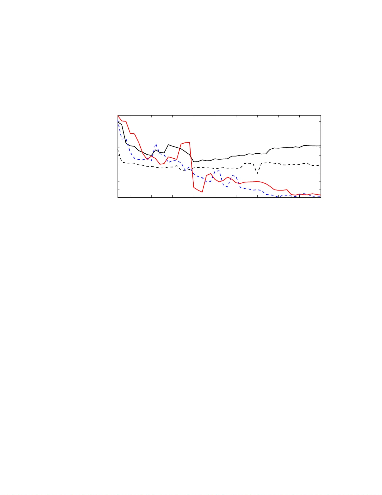
Electronic Journal of Stati stics ISSN: 1935-7524 Predictio n of m ultiv ariate resp onses with a select n um b er o f principal comp onen t s Inge Ko c h Scho ol of Mathematics and Statist ics University of New South Wales Au str alia e-mail: inge@ unsw.edu .au and Kan ta Naito Dep artment of Mathematics Shimane University Jap an e-mail: naito@riko.sh imane-u. ac.jp Abstract: This paper proposes a new method and algorithm for predicting multiv ariate responses in a regression setting. Research in to classification of High Dimension Lo w Sample Size (HDLSS) data, i n particular microar- ray data, has made considerable adv ances, but regression prediction for high-dimensional data wi th con tin uous resp onses has had less atten tion. Recen tly Bair et al (2006) proposed an efficien t pr ediction method based on supervised principal componen t regression (PCR). Motiv ated by the fact that a larger num ber of principal comp onen ts resul ts in better regression perf ormance, this pap er exte nds the m ethod of Bair et al in sev eral wa ys: a comprehensive v ariable ranking is combined with a selection of the best n umber of components for PCR, and the new metho d further extends to re- gression with multiv ariate resp onses. The new m ethod is particularly suited to HDLSS problems. Applications to simulated and real data demonstrate the p erformance of the new method. Comparisons with Bair et al (2006) sho w that for high-dim ensional data in particular the new r anking results in a smaller n umber of predictors and smaller errors. AMS 2000 sub ject classi fications: Pri mary 62J99; secondary 62H99. Keywords and phrases: Di m ension Selection, Mul tiv ariate Regression, Multiv ariate Responses, Principal C omp onent Regression, V ari able Rank- ing, V ari able Selection. 1. In tro duction Classification of high-dimensional data – motiv ated mainly by the imp ortance of tumor classificatio ns for high-dimensional microa rray da ta – has attra cted m uch recent attention. T o date les s attent ion has b een paid to the prediction of surviv al times for gene expr ession data, although s uch prediction can pro- vide v aluable a dditional knowledge and impor tant information in the selection 1 imsart-e js ver. 2008/01/24 file: ejs_2008_278.te x date: March 2, 2022 Ko ch & Naito/Pr e diction wit h a sele ct numb er of c omp onents 2 of relev ant g enes. O ne imp ortant adv a nc e in this area is Bair et al ( 2006) who prop osed a prediction metho d for m ultiple reg ression based on sup ervised princi- pal comp onents. They prop ose d not only a new metho d, but also an underlying mo del based on la tent v ariables which provides a g o o d and theo r etically founded explanation of their metho d. In this pap er we fo cus on predictio n of co n tin uo us r esp onse v ariables in a very gene r al linear r egressio n framework and extend the research of Bair et al (2006) in a n umber o f c r ucial wa ys. Like Bair et al we allow a very lar ge nu m ber of pr e dictors, but in addition we cons ider multiv ariate rep onses as met in practice, for example, in the prediction of treatmen t pla cement and facilities in drug related offences. Including m ultiv ar iate resp onses in our mo de l is a genuine extens ion ov er Bair et al whose approa ch c a nnot handle such data. A central problem in linea r reg ression fro m multiv ar iate predictor s is the choice o f v ariables that are included in the pr ediction mo del. Section 2 briefly reviews the classical case and principal compo nen t r egressio n (PCR). F or hig h- dimensional data PCR has a n in uitive appeal for regr ession prediction, and w e follow that path - similar to B air et al (2006). But unlike their appr oach, which uses the first principal comp onent only , we in tegr ate the dimension selection of Ko ch and Naito (2007 ) into PCR, whic h yields a b etter fit bas ed on more than one principal co mp onent. Compared to Bair et al , our predictio n mo del is mor e complex and extensive; our choice of dimension has a theore tica l foundation, and sinc e w e use more than one pr e dictor, our prediction mo del results in mor e accurate prediction. Another prediction method with applications in chemometrics has b een pro- po sed in Gustafsso n (2005 ). This approach also falls into the PCR fra mework but then uses a further rota tion of the sphered principa l comp onents. F or re - gressio n pr edictions such rotations hav e no effect, since they would cancel o ut in an appropriate verson of (5 ). F or this reason we compare our results to those of Bair et al (20 0 6). A key issue in class ification a nd prediction of a contin uous resp onse v ariable from high-dimensio nal data is the preselection of a mo de r ate num b er of v aria bles that hav e strong predictive p ow er. In microa rray analysis this first selectio n is often achieved b y univ ariate t- tes ts. Bair et al (2006) replac e these tests, essen- tially by calcula ting the univ ariate corr elation co efficient b etw ee n each predictor and the resp onse v ar iable, and mak e a pr eselection o f the v ar iables based on the absolute v a lue o f these cor relation co efficients. This prese le ction is simple to im- plement and understa nd, but do es not capture the in teraction of the v ariables or genes . W e address the pres election problem a nd prop os e a rank ing of the v ariables which ta kes into acco un t all predictors simultaneously , a nd th us takes care of v aluable interaction b etw een the v ariables in the pre selection. Our prediction metho d can b e regarded as a tw o-step v a riable selection. The first step s e le cts the v aria bles that are most imp or tant for prediction, while the second step summarises thes e v ariables in a smaller, and judiciously chosen, nu m ber of comp onents. The pap er is organis ed as follows. Section 2 r eviews regres sion prediction, and describ es v ar iable ra nk ing based on a canonical cor r elation approa ch. Section imsart-e js ver. 2008/01/24 file: ejs_2008_278.te x date: March 2, 2022 Ko ch & Naito/Pr e diction wit h a sele ct numb er of c omp onents 3 3 prop oses our regres sion algorithm which is based on v ariable r anking and di- mension sele ction. Section 4 provides more details and prop er ties of our v ariable selection, a nd includes compa r isons with the metho d of Bair et al (2006). Sec- tion 5 shows how our metho d per forms in practice fo r sim ula ted and real data, including an exa mple of high-dimensional microar r ay data, a nd gives compar - isons with the approach of Ba ir et al (2006). W e c o nclude with a discussion o f our metho d a nd a lgorithm in Section 6. 2. Prediction and Canoni cal Co rrelations 2.1. R e gr ession Pr e dicti on W e co nsider the multiv ar iate regr e ssion setting: Y = XB + E , (1) where Y = [ y 1 · · · y N ] T denotes the ma trix o f res po nses, and, each resp onse y i is a v ector of length q . F urther , B = [ β 1 · · · β p ] T is the p × q matrix o f co efficients, and E is the N × q error matrix. The design matrix is the same a s in a m ultiple regres s ion setting: X = [ x 1 · · · x p ] , so eac h v ariable o r feature vector x j is o f length N . Throughout this pap er w e will assume that the co lumns of X are centred. An estimator for B is given by b B = ( ˜ X T ˜ X ) − 1 ˜ X T Y , (2) where ˜ X is derived from X , a nd a new q - dimens ional res po nse b y is predicted for a single p -dimensional datum x 0 by b y T = x T 0 ( ˜ X T ˜ X ) − 1 ˜ X T Y . (3) If p < N and ( X T X ) − 1 exists, then ˜ X = X leads to an estimator and new predictions based on all v ar iables. If the inverse ( X T X ) − 1 do es not exist or is unstable, then a s mo o thed or pena lised inv er se as in ridge reg ression or the more r ecent lasso - see Hastie et al (2007 ) or Meier and B¨ uhlmann (2007) and references there in - is commonly used. In this pa per we shall not b e concerned with such in verses. In mult iple linear r egressio n the aim is to r educe the num b er of v ariables. Without go ing into the differ e n t metho ds of finding such subs ets of v aria bles, but assuming instead one has found a subset X − where the super script − indicates that some v ar iables are omitted, then ˜ X = X − and ˜ x 0 = x − 0 in (2) a nd (3). PCR does not leav e o ut v ariables, but uses weighted sums of all v ar iables, with weigh ts allo ca ted a ccording to the contribution to v a riance of the v aria bles. Let Z ( k ) = X Γ k = [ z 1 · · · z k ] . (4) Then Z ( k ) is an N × k matrix, with k ≤ p , Γ k denotes the ma tr ix whic h c o nsists of the first k eig env ectors of the sample cov ar iance matr ix of the predictors, and imsart-e js ver. 2008/01/24 file: ejs_2008_278.te x date: March 2, 2022 Ko ch & Naito/Pr e diction wit h a sele ct numb er of c omp onents 4 the i -th column vector z i is obtained by pro jecting X on to the i -th eigen vector γ i of Γ k . In the PCR setting ˜ X = Z ( k ) and ˜ x 0 = z ( k ) 0 , and one obtains the estimator b B and predicto r b y g iven by b B =  Z ( k ) T Z ( k )  − 1 Z ( k ) T Y =  Γ T k X T X Γ k  − 1 Γ T k X T Y and b y T = x T 0 Γ k  Γ T k X T X Γ k  − 1 Γ T k X T Y . (5) Since z 1 is a linear co m bination of a ll v ariables, k = 1 is often used in PCR, for example in Bair et al (200 6). This first principal compo nen t often do es not sufficiently summarise the predictors, and then it is impo rtant to find an appropria te v a lue for k . W e return to this c ho ice in Section 3.5 .2. 2.2. V ariable R anking and Canoni c al Corr elations In univ ariate regr ession the cor relation coefficie nt ρ of X and Y is defined by ρ = cov ( X , Y ) p v ar [ X ] v ar [ Y ] , (6) where cov refers to the cov ariance and v ar to the v ariance. F or reg r ession, this co efficient rela tes the standar dised resp onse and predictor v ariables. In m ultiple linear reg ression the absolute v alue of the correlatio n co efficient can b e used to order the predicto r v ariables according to the strength of their correla tion with a univ ariate r e s po nse Y , so [ x 1 · · · x p ] →  x (1) · · · x ( p )  where the vectors x ( i ) are ordered such that | ρ (1) | ≥ | ρ (2) | · · · | ρ ( p ) | , and ρ ( i ) denotes the correlatio n betw een a resp onse vector y and x ( i ) . As po int ed out in Section 1, the correla tion co efficient takes into account one fea ture vector at a time - so c o nsiders only the marginals - and cannot account for any interaction betw een the x j s. F urther, the correlatio n co efficients and the ab ov e or dering do not extend to m ultiv ar iate resp onses. F or a m ultiv ar ia te pre dictor X and a m ultiv ar iate r esp onse Y a na tural generalisa tion of ρ is the ma trix of canonica l c o rrelatio ns C = Σ − 1 / 2 X Σ X Y Σ − 1 / 2 Y , (7) which r eplaces the univ ar iate cov ( X , Y ) of (6) by the p × q co v ar iance matrix Σ X Y of X and Y , and each of v a r [ X ] and v ar [ Y ] by their r e s pec tive v aria nce matrices Σ X and Σ Y . The matrix C is commonly used in cano nical correlatio n analysis, and contains information ab out the strength of the relations hip o f the individual v ariables . F or a univ ariate resp ons e Y , the matrix C reduce s to a p × 1 v e c tor whose entries give rise to an o rdering or ranking of the p v ariables of X which makes use of all interactions of the data. In Step 1 of our alg orithm we show ho w the matrix C induces a a r anking of the data v a r iables which als o applies imsart-e js ver. 2008/01/24 file: ejs_2008_278.te x date: March 2, 2022 Ko ch & Naito/Pr e diction wit h a sele ct numb er of c omp onents 5 1. to multiv a riate resp ons es Y , and 2. to data who se dimension p exceeds the sample s iz e N . 3. A R egression Algori thm Based on Ranking and Dimensio n Selection 3.1. The Underlying L atent V ar iable Mo del The mo del for a single resp onse vector y is y = W T s + δ , (8) where W T is a q × H matrix, s is an H × 1 latent vector with non-Gaussia n comp onents, H ≪ p , and δ is a q × 1 err or vector. Let I deno te a prop er subs et of { 1 , ..., p } and set | I | = m < p . F or i ∈ I , the i -th feature of the input vector x is mo delled by x i = p T i s + η i , (9) where the p i s are H - dimensional vectors, the η i are error s, and H ≤ m . Com- bining (8) and (9), w e hav e  x ∗ y  =  P W T  s +  η δ  , (10) where x ∗ is a m × 1 subv ector of x defined b y the compone nts o f (9) and P is a m × H matrix having p T i ( i ∈ I ) as its rows. T he m -dimensiona l vector x ∗ contains the feature s which are mos t relev ant for prediction a nd which are mo delled by a smaller n um b er H of laten t v aria bles. Step 1 of the algorithm shows how w e obtain the v ector m , and Step 2 elucidates the c ho ice of H . 3.2. V ariable R anking with C W e beg in with a n ins pectio n of the matrix C given in (7) which can b e re g arded as a m ultiv ar iate corr elation coefficient of size p × q . T o be able to rank the v ariables of X , we use the fact that the str ongest correlation b etw een the X and Y v ariables is g iven by the larges t eig env alue, κ 1 , of C . The first left and right eigenv ec tors of C , denoted by h 1 and g 1 resp ectively , satisfy C g 1 = κ 1 h 1 . (11) F urther the entries of h 1 and g 1 contain relative w eig hts for the v ar iables of X a nd Y (see Theo rem 3.6 , Chapter 3 of Ko ch (2009)). Next obs erve tha t the correla tion coefficie nt ρ rela tes the univ ar iate standardis ed v ariables X and Y via Y /σ Y = ρX/σ X , where σ Y and σ X is the standard devia tion of Y a nd X , resp ectively , and b oth X and Y are assumed to be ce ntred. The m ultiv aria te analogue of this r elationship is Σ − 1 / 2 Y Y = C T Σ − 1 / 2 X X or eq uiv a le n tly Y = ˜ C T X , (12) imsart-e js ver. 2008/01/24 file: ejs_2008_278.te x date: March 2, 2022 Ko ch & Naito/Pr e diction wit h a sele ct numb er of c omp onents 6 where ˜ C = Σ − 1 / 2 X C Σ 1 / 2 Y = Σ − 1 X Σ X Y . Combining (11) and (12) w e note tha t C applies to the s pher ed data while ˜ C applies directly to the raw data . P ut b = 1 κ 1 Σ − 1 / 2 X C g 1 , (13) and observe that b is the first (left) canonical c ov ar iate vector (see Chapter 3, Ko ch (20 09)). Ranking of v a r iables is particula rly imp ortant for HDLSS data, when the nu m ber of v ariables exceeds the num b er o f obs erv ations. In this case the usual estimate of the cov ariance matrix Σ X is not in vertible. Assume that X ha s rank r (with r ≤ min( N , p )). Let X = UL V T (14) denote the s ingular v alue decomp osition o f X where U and V ar e N × r a nd p × r matrices, resp ectively , bo th with o r thonormal co lumns, and L is the r × r diagonal matrix with singular v alues a s its entries lis ted in decr easing order. F or nota tional co n venience w e deno te the sample version of C by b C . Co m- bining (7) and (14) we o bta in b C =  X T X  − 1 / 2  X T Y c   Y T c Y c  − 1 / 2 = VU T Y c  Y T c Y c  − 1 / 2 , (15) where Y c is the centred Y . Similarly , the sample version b b of the vector b in (13) is calculated b y b b = 1 b κ 1  X T X  − 1 / 2 b C b g 1 = 1 b κ 1 VL − 1 U T Y c  Y T c Y c  − 1 / 2 b g 1 , (16) where b C b g 1 = b κ 1 b h 1 is the sample version of (11) with b κ 1 and b g 1 the first eigen- v alue and r ight eigenvector resp ectively . The expressio ns (15) and (1 6) do no t depe nd o n the relationship b e t ween p and N , s o can be eq ually applied to con- ven tional data with p < N as w ell as to HDLSS data. 3.3. Pursui t of Inter esting D imensions Since the 197 0s and more particular ly since F r iedman and T uk ey (1 974), sub- spaces in data a re regarded ‘uninteresting’ if they ar e random or unstructured, and c o nv ersely , a pro jection, or subspace is int eresting if it is far from Gaus- sian. F ollowing these ideas for a given data structure X , which could denote the o riginal data, ra nked data or a subset of the v aria bles of the original data, we aim to find the subspace of those v aria bles of X which co n tain in teresting non-Gaussian structure. The first principal comp onent do es no t no r mally con- tain enough structure, since it is one- dimensional , w hile the whole data contain structure a nd randomness. The go al is thus to sea rch for a low-dimensional subspace which con tains the essential information in the da ta. Two clo sely rela ted metho ds, Pro jection Pursuit and Independent Compo- nent Analysis, find non-Gaussian pro jections in data. See Hub er (19 85), J o nes imsart-e js ver. 2008/01/24 file: ejs_2008_278.te x date: March 2, 2022 Ko ch & Naito/Pr e diction wit h a sele ct numb er of c omp onents 7 and Sibson (198 7), F riedman (19 87) and Hyv¨ ar ine n, et al (200 1) for g o o d a c- counts o f ho w to find o ne or more pro jections. More recently Scholz et al (2004 ) and Ko ch and Naito (2007) pro p os ed meth- o ds for determining the num b er of these pr o jections or the dimension of the subspace. Mo tiv ated by their sub-Gaussian metabolite data, the ‘optimal’ di- mension in Scholz et al (2 004) is that whic h r esults in the highest num b er of independent comp onents with negative kurtosis. Ko ch and Naito (200 7 ) use kurtosis a nd skewness for their dimensio n s election metho d which is generally applicable and has a theor etical foundation. F or this r eason w e will a pply their criterion in the pur s uit o f the b est subspa ce dimension. W e briefly rev iew the relev ant parts o f their metho d and r e late their theoretica l r esults in Sectio n 4.3. Ko ch a nd Naito’s star ting p oint is the observ ation that the most interesting low er-dimens io nal subspace is that in which the la rgest devia tion fro m the Gaus- sian can b e obtained. An appropria te measure, which can b e calcula ted dir ectly from the data, is kurtosis. Let x p,j with j = 1 , . . . , N denote p -dimensio nal ob- serv ations, here rega rded as columns of X T . The sample kurtosis b β is defined by b β ( X ) = b β ( x p, 1 , ..., x p,N ) = max α ∈U p − 1 b B ( α | x p, 1 , ..., x p,N ) , (17) where b B ( α | x p, 1 , ..., x p,N ) =      1 N N X i =1  α T ( x p,i − x p ) √ α T S α  4 − 3      , U p − 1 is the unit sphere in R p , S is the sample cov ariance of X , and x p is the sample mea n which is zero due to centring o f X . F or 2 ≤ k ≤ p , put ˜ Z ( k ) = Z ( k ) Λ − 1 / 2 k with Z ( k ) as in (4) and Λ k the cov ariance matrix of Z ( k ) . W e calculate the sample kurtosis of the ˜ Z ( k ) , deno ted by b β k ( ˜ Z ( k ) ). The most non-Gaussian dimension is the H whic h satisfies H = a r gmax 2 ≤ k ≤ p ( r N 4! b β k ( ˜ Z ( k ) ) − τ k ) , (18) where τ k is a certain co nstant used for bias-adjustment. The choice of the most non-Gaussia n dimension in Ko ch and Naito’s metho d requires a sequence of subspaces o f dimensions 1 < k ≤ p . Pr incipal comp onent analysis (PCA) do es pr ovide s uch a seq uence, but P CA is base d purely on v ariance, and may therefore exclude v ariables that are imp or tant for regress ion prediction. F or this reas on, we cannot apply their cr iterion direc tly to the k - dimensional sphered P C data. Step 2 of our algor ithm shows how the selection is achiev ed in a regres s ion fra mew ork. Details r elating to the choice of τ k are given in Sectio n 4.3. 3.4. A R e gr ession Algorithm In this sectio n w e present our alg orithm which cons ists of three s teps. Step 1 achiev es v aria ble ranking which plays a n imp ortant role in our algo rithm and is one of the re asons why the phrase sup ervise d can b e used. imsart-e js ver. 2008/01/24 file: ejs_2008_278.te x date: March 2, 2022 Ko ch & Naito/Pr e diction wit h a sele ct numb er of c omp onents 8 An effectiv e dimension reduction metho d is applied in Step 2 a nd pr ediction as describ ed in (5) is accomplished in the final Step 3 . 3.4.1. Step 1 Let [ X Y ] denote the predicto r and resp onse v aria bles which satify (9) and (8). Let b C a nd b b de no te the ranking matr ix and ranking vector obtained from [ X Y ] as in (15) and (16). F o r m = 2 , . . . , p let | b b j 1 | ≥ | b b j 2 | ≥ · · · ≥ | b b j m | denote the m lar gest entries (in absolute v alue) of b b , r anked in decreas ing or der, and define the m -dimensional ranked data X m = [ x j 1 · · · x j m ] =    x T m, 1 . . . x T m,N    (19) where the i -th v ariable is the v ar iable corres po nding to the i -th larg est ent ry b b j i of b b . Our notation indicates that the column vectors x j i are feature vectors while the row vectors x T m,k corres p ond to the N observ a tions. 3.4.2. Step 2 F or m = 2 , . . . , min( N , p ) apply principal co mpo nen t analysis to X m . Sphere the principal co mpo nen ts to obtain the N × m ra nked and sphered PC data S m = X m ΓΛ − 1 / 2 , (20) where N − 1 X T m X m = ΓΛΓ T denotes the sp ectral decomp osition with the eig en- v alues in Λ a r ranged in decr e asing order, Γ is the ortho g onal matrix who se columns are eig env ectors be lo nging to the e lemen ts of Λ . F or m and the ranked and sphered PC data S m calculate the sample kurtosis b β k ( X m Γ k Λ − 1 / 2 k ) for each k ≤ m , with Λ k the appr opriate cov a riance matrix, and determine the dimension H = H ( m ) as in (18). Put e X m,H = X m Γ H , where Γ H denotes the firs t H columns of Γ , and so e X m,H is the matrix which consists of the first H principal comp onents o f X m . 3.4.3. Step 3 F or m = 2 , . . . , min( N , p ) and a typical expla na tory v ariable z ∈ R p predict the q -v aria te b y as in (3) fro m the ranked data X m : b y T = z T m Γ H  e X T m,H e X m,H  − 1 e X T m,H Y = z T m Γ H  Γ T H X T m X m Γ H  − 1 Γ T H X T m Y , (21) where z m is a subvector of z containing the fir st m ranked v ar iables as defined in (19) in Step 1. imsart-e js ver. 2008/01/24 file: ejs_2008_278.te x date: March 2, 2022 Ko ch & Naito/Pr e diction wit h a sele ct numb er of c omp onents 9 4. Some Prop erties 4.1. R emarks on the Mo del and Algorithm 4.1.1. R emarks on Step 1. Our mo del is based on a set o f features X ∗ which are descr ibed by X m in the algorithm. This means obtaining X m from X via b C is equiv alent to finding the set of indices I which c haracteris e X ∗ . In addition to the rank ing with b b we also rank the data with the vector b h 1 which is the sa mple version of h 1 in (11); see also (16). If a distinction b etw een these tw o rank ing schemes is required we put b b 1 = b b and b b 2 = 1 b κ 1 b C b g 1 = b h 1 . Although b b 1 and b b 2 will lead to differen t submatrices X m , the rest of our algorithm pro cee ds in the sa me wa y for both ranking schemes. A compariso n betw een the tw o ranking vectors shows that, apar t from the sca le factor 1 / b κ 1 , b b 1 contains sphering with  X T X  − 1 / 2 , therefore applies to r aw o r cent red data, while b b 2 could b e int erpreted as applicable to data where sphering is not required or appropria te. With very large data sets in par ticula rly , it is not clear whether the spher- ing comp onent is required, and we therefore prop os e to use b oth versions in applications. Our ra nking extends the ranking prop osed by Bair et a l (2006) which is essentially based o n the cor r elation co efficient b etw een the univ ariate resp onse and each feature vector. W e will return to these ranking sc hemes in Section 4 .2. 4.1.2. R emarks on Step 2. The ranked feature set X m is generally still too lar g e to find the ‘b est’ non- Gaussian predictors co rresp onding to s in (10). W e use dimension reduction with PCA to pursue the b est no n- Gaussian subspace. Using the notation of (20), we deno te the eigenv a lues of N − 1 X T m X m by λ 1 ≥ λ 2 ≥ · · · ≥ λ m ≥ 0, and the eigenv ectors by Γ = [ γ 1 · · · γ m ]. It follows that N − 1 X T m X m γ j = λ j γ j j = 1 , ..., m, (22) and hence N − 1 X T m X m = m X j =1 λ j γ j γ T j = H X j =1 λ j γ j γ T j + m X j = H +1 λ j γ j γ T j . In Step 2 w e c ho o s e the cut-off ‘ H ’ o f (18) as in Ko c h and Naito (2007); so H is the dimensio n which y ields the most no n-Gaussian pro jection. F or this selection of H we obtain e X m,H = X m Γ H . F urther, by applying (18) to subs pa ces o f the ranked rather than the or iginal data, the most non-Gaussia n dimens ion is determined from a mongst the v ariables that are imp o rtant for prediction. imsart-e js ver. 2008/01/24 file: ejs_2008_278.te x date: March 2, 2022 Ko ch & Naito/Pr e diction wit h a sele ct numb er of c omp onents 10 4.1.3. R emarks on Step 3. Instead of (1) we consider the m ultiv aria te regres s ion mo del Y = e X m,H B r + E , (23) where B r is the H × q matrix of co efficients for s ubsets of the ranked data, a nd E denotes the er rors. The estimate of B r corres p onding to (2) is b B r =  e X T m,H e X m,H  − 1 e X T m,H Y . Hence for a datum z , we extract the subv ector z m whose comp onents corresp ond to the indices { j 1 , ..., j m } obtained in Step 1. The prediction for z via the mo del (23) is o btained by b y = b B T r Γ T H z m , which is nothing other than (21). Note that we can also express b y in terms of the eig env alues and eig env ectors of N − 1 X T m X m as follows: b y = 1 N H X j =1 1 λ j Y T X m γ j γ j T z m . (24) 4.2. Pr op erties of b b F or univ ar iate resp onses, so q = 1, the r egressio n mo del (1) r educes to y = X β + ε , (25) where y is the N × 1 resp onse vector, β is the p × 1 co efficient v e c to r, and ε is the N × 1 er ror vector. In this case, fr om (15), b C =  X T X  − 1 / 2 X T y c ( y T c y c ) − 1 / 2 , and hence we hav e b h 1 = 1 q y T c X ( X T X ) − 1 X T y c  X T X  − 1 / 2 X T y c , where y c is the centred resp onse. Therefor e it follows that b b =  X T X  − 1 / 2 b h 1 ∝  X T X  − 1 X T y c ≡ b β . (26) It is well known that b β is characterised as the vector β which maximises the co r relation b e t ween y and X β (see Section 10.2.1 of Mar dia et al , 1 979). Moreov er any scalar mult iple of b β a lso ma ximises the correlatio n. Therefore using b b is essentially eq uiv alent to using b β in our v ariable ranking since a scala r m ultiple do es not affect the ranking. F or q = 1 w e a ctually use b b 1 = b β and b b 2 =  X T X  1 / 2 b β . imsart-e js ver. 2008/01/24 file: ejs_2008_278.te x date: March 2, 2022 Ko ch & Naito/Pr e diction wit h a sele ct numb er of c omp onents 11 W e compare ranking with b b to that used in Bair et al (2006). Our method for choosing relev ant predictors is bas ed on the full canonical correlatio n matrix b C betw een the predictors and the resp onses, or the full LSE . In contrast, Bair et al (2006) use cor r elation co efficients or separa te LSEs for the univ ar ia te resp ons e and each univ aria te feature with a mo del similar to (10). This corresp onds to cons idering only the marginals, while ig no ring interactions, and admits the int erpretation of a single LSE under the simplified linear model y = β j x j + ε for j = 1 , . . . , p, where ε is an err or vector with mean zer o and v ariance σ 2 I N . In other words, they apply simple regr ession with x j as a single predictor , although their un- derlying setting is that of m ultiple r egressio n (25). They use s j = x T j y / || x j || , with j = 1 , ..., p , for their ranking, which can b e obtained as a standardised LSE of the β j s. Bair et al implement their so rting in an analogo us w ay to Step 1 of our algo rithm, and their thresho ld, which corres po nds to the c ho ic e of m in our setting, is chosen by cr oss-v alida tio n. Next we br iefly examine prop er ties of the s j s. Under the usual manipulations conditional on x , it follows that E [ s j ] = 1 || x j ||   || x j || 2 β j + X i 6 = j x T j x i β i   , v ar [ s j ] = σ 2 . In particular, this calculation shows that s j is not un bia sed for β j . On the other hand, since b b 1 = [ b b 11 · · · b b 1 p ] T = b β , E h b b 1 j i = β j , and v ar h b b 1 j i = σ 2 d j j , where d kℓ is the ( k, ℓ )-th comp onent of  X T X  − 1 . No te that b b 2 is not un bia sed, but the v ar iance of ea ch of its comp onents is σ 2 . F or p fixed, standard a symp- totic theory suggests that  X T X  − 1 = O p ( N − 1 ) a s N grows, a nd thus b b 1 j can estimate β j more accurately than the bia sed s j in the selection of relev ant pre- dictors. It is also int uitiv ely obvious that v aria ble selection should include the correla tion structur e from all pr edictors. A further adv antage o f our ranking method over the selection of v ariables with s is that the b b -ranking is a pplicable to m ultiv ar ia te res po nse v ariables, while there is no obvious ex tension of s to a truely multiv a riate setting. Since b b tak e s in to account the who le cor relation structure, computations a re more complex a nd mo re inv olved than tho s e res ulting in the calculatio ns of the s j s. The latter can b e carried out very efficien tly for any num b er of features as the complex ity only gr ows with the n um ber of v ar iables. Cho osing b etw een these t wo ra nking schemes therefore represents a compromise b etw een computational efficiency and ex ploitation of the co rrelation structure. imsart-e js ver. 2008/01/24 file: ejs_2008_278.te x date: March 2, 2022 Ko ch & Naito/Pr e diction wit h a sele ct numb er of c omp onents 12 4.3. Detail s on the D imension Sele ction F or 2 ≤ k ≤ p and ˜ Z ( k ) = Z ( k ) Λ − 1 / 2 k as in (18) of Sectio n 3.3, b β k ( ˜ Z ( k ) ) increases with the dimensio n k . This means that dir ect use of b β k ( ˜ Z ( k ) ) is not useful for the selection o f the b est k . Mimicking the deriv a tion of the AIC and using some insight ab out null str uc- ture motiv ate us to consider the b ehaviour of r N 4! b β k  ˜ Z ( k )  under the k -dimensional standar d Gaussian structur e (see Sections 3.1 and 3.2 in Ko ch a nd Naito, 200 7). Under Gaussian assumptions it is shown that r N 4! b β k  ˜ Z ( k )  → T k in distribution as N → ∞ , and hence als o that E " r N 4! b β k  ˜ Z ( k )  # ≃ E [ T k ] for la rge N , wher e T k is the ma xim um o f a ze r o mea n Ga ussian r andom field on U k − 1 . The quantit y E [ T k ] cannot b e calc ula ted directly , but is estimated via the bo unds be low, her e only given for kurtosis and a djusted to our s c enario. Theorem [Ko ch and Naito (2 007)] F or e ach k ≤ min { p, N } LB k ≤ E [ T k ] ≤ UB k wher e LB k = k − 1 X e =0 ,e : even ω k − e Λ k − e,ρ − k + e (tan 2 θ ) , UB k = LB k + √ 0 . 6 E [ χ ρ ] [1 − Ψ( θ , k )] . Since the lower b ound L B v anishes r apidly with dimension, K o ch and Naito contin ue with upp er bound UB . The interested reader is referred to their pa- per for details o n the lower bo und. In the no tation o f their theorem, θ = cos − 1 ( √ 0 . 6), Ψ is a weight ed sum o f upper tail probabilities of the beta dis- tribution, a nd χ ρ denotes a χ -distributed r andom v aria ble with ρ degrees of freedom and ρ =  k +3 4  . Go o d approximations for the v alues of UB k are given in Ko ch and Naito (2 0 07), and are denoted by d UB k . Ko ch a nd Naito prop ose to use these ta bulated v alues as the constant τ k in (18). Returning to the notation in Section 3.4 .2, Step 2, we imsart-e js ver. 2008/01/24 file: ejs_2008_278.te x date: March 2, 2022 Ko ch & Naito/Pr e diction wit h a sele ct numb er of c omp onents 13 • define, for k ≤ m , the bias adjusted version b I k of b β k by b I k = r N 4! b β k ( X m Γ k Λ − 1 / 2 k ) − d U B k , • and take H ( m ) = ar g max 2 ≤ k ≤ m b I k , as the practica l dimension selecto r of the ranked m -dimensional data S m consisting of N samples. The theorem a nd the practical dimensio n s elector show that the dimensio n H ( m ) is that for whic h the difference to the Gaussian is maximal. 4.4. A Gener al Vi ew of Sup ervise d Pri ncip al Comp onents In this section we clarify why our a lgorithm can b e rega rded as a generalisation of the ‘Predictio n b y sup ervis ed principal comp onents’ prop osed by Bair et al (2006). Like our metho d, theirs starts with X m , whic h they obtain by their simpler v ar ia ble ranking de s crib ed in Subsection 4.2 . W e express the singular v alue decomp osition (14) of X m in terms of the individual eigenv alues and eigenv ector s and o btain X m = [ u 1 · · · u m ] diag n p d 1 , ..., p d m o    v T 1 . . . v T m    , where, for j = 1 , ..., m , the d j s, u j s and v j s satisfy X T m X m v j = d j v j , X m X T m u j = d j u j , X m v j = p d j u j (27) In equations (6) and (7) of their Section 2.1 , Bair et al (200 6) describ e their prediction b y spc in a multiple regressio n mo del such as (25). F o r a given datum z m , and using our notation, this is essentially b y spc =  u T 1 y  z T m  1 √ d 1 v 1  = z T m  1 √ d 1 v T 1 X T m y   1 √ d 1 v 1  = z T m  1 d 1 v 1 v T 1  X T m y = 1 N λ 1 y T X m γ 1 γ T 1 z m , (28) where the last equality can b e seen using (22) and (27). C o mparing (24) with (28), we see that b y spc corres p onds to the case H = 1 in (24), and the pr e dic tio n in (24) is q -dimens io nal, while b y spc is one-dimensiona l. In this sense our prediction is a natural genera lisation of the method discusse d by Bair et al (2006) to m ultiv ariate resp onse s , w he r e q ≥ 2 . imsart-e js ver. 2008/01/24 file: ejs_2008_278.te x date: March 2, 2022 Ko ch & Naito/Pr e diction wit h a sele ct numb er of c omp onents 14 5. Results This sectio n rep orts on the numerical per formance of our algorithm and co m- parisons of our method with that of Ba ir et al ( 2006). F o r the simulated data and the real data sets we predict b y . T o assess and compare the per formances o f the different metho ds we use the least squa r es error criterio n LSE( m ) = ( 1 N N X i =1 || b y i − y i || 2 ) 1 / 2 (29) where m is n umber o f v ariables of the ranked subma trix X m . In Figures 1-5 w e will adhere to the following no tation on metho ds: 1. kn b1-p cH : r anking with b b 1 follow ed b y PCR with H = H ( m ) selected comp onents; 2. kn b2-p cH : r anking with b b 2 follow ed b y PCR with H = H ( m ) selected comp onents; 3. bhpt-p cH : ra nking as in Bair et al (20 06) follow ed by PCR with H = H ( m ) selected c o mpo nent s; 4. bhpt-p c1 : ranking as in Bair et al (2006) follow e d by PCR with the first comp onent only; 5. nr-p cH : PCR with H = H ( m ) selected compo nent s based on the orig ina l data without r anking. Here ‘p cH’ refers to Steps 2 and 3 of our a lgorithm, and ‘pc1 ’ refer s to the prediction step of Bair et al (2006). W e ha ve added tw o other prediction meth- o ds, bhpt-p cH and nr-p cH. The first, bhpt-p cH, is a mix tur e of o ur metho d and tha t of Ba ir et al ; it uses r anking a s des crib ed in B a ir et al (200 6), but then applies Steps 2 and 3 of our algo rithm. The las t, nr-p cH, is only used in Example 3.2.1, and will be describ ed further there. Like bhpt-p cH, it is used to assess the a dv a ntages of our v aria ble ranking. W e ca lculate the predicted v alues b y and the err or (29) for m ≥ 2. In ea ch case we indicate whic h of the five metho ds have b een use d. W e show p erfor mance plots with m on the x -axis, a nd LSE on the y -axis. 5.1. Simul ate d Data Based on mo del (10) w e generate t wo sets of da ta. The firs t refers to a class ical m ultiple r egressio n framework, and the second mo dels a high dimension low sample size (HDLSS) general m ultiv ariate r egressio n setting. F or b oth mode ls w e us e the 3 -dimensional source vector s = [ s 1 s 2 s 3 ] T whose comp onents are independently distributed as follows: s 1 ∼ uniform on[0 , 1], s 2 ∼ Exp onential with mean 1, and s 3 ∼ N (0 , 1), the standar d Gaussia n. So H = 3 in the mo del. F o r the terms δ a nd η we use vectors with independent components distributed as 0 . 5 × N (0 , 1 ), in q dimensions for δ and in m dimensions for η . The v alues for q and m will b e differen t in the tw o settings as will be the transformatio ns P a nd W . imsart-e js ver. 2008/01/24 file: ejs_2008_278.te x date: March 2, 2022 Ko ch & Naito/Pr e diction wit h a sele ct numb er of c omp onents 15 Example 5.1 . 1: Classical Data with q = 1 , p = 13 and N = 172. W e us e the matrices P =   I 3 2 I 3 3 3 3   (30) and W T = [4 − 3 − 2 ] , where I d denotes the d × d identit y matrix. The predictor is co nstructed by stacking x T = [ x T ∗ x T L ] where x L is a 6-dimensional vector, and each of the 6 comp onents is genera ted indep endently as 0 . 5 × N (1 . 5 , 1). Since the matrix P gives rise to m = 7, the pr e dictor vector ha s 13 dimensions. W e gener ate 172 predictors a nd resp onses , and combine them to form one data set D = { ( y 1 , x 1 ) , ..., ( y 172 , x 172 ) } . In the sim ulations we use 10 0 such data sets D j . F or each data set D j we calculate the predicted v alues b y a nd the er ror (29) for m = 2 , . . . , 13 and each of the four pre diction metho ds k n b1-p cH, knb2-pcH, bhpt-p cH and bhpt-pc1. Figure 1 shows the p er fo rmance of the four metho ds for a typical simulation. 2 3 4 5 6 7 8 9 10 11 12 13 0.8 1 1.2 1.4 1.6 1.8 2 2.2 2.4 2.6 Fig 1 . LSE v ers us dimension for si mu lated data; knb 1-pcH (red), knb 2-pcH (blue), bhpt-p cH (blac k dashed) and bhpt-p c1 (black ). The x -axis displays the dimension m of X m and the y -a xis shows the LSE as in (2 9). All 10 0 simulations show that prediction with H compo nents out- per forms prediction with the first comp onent only , as se e n in this figur e. Using H co mpone nts leads to a strong decrea se as dimenion increases and then the curves flatten out. In some cases, a s for knb1-pcH in Figure 1 , the curve has a minim um (here at 5) and then increases again. This behaviour is not uncommon and shows clearly that p erforma nc e is not improv ed w ith more v ariable s . The next figure (Figure 2) examines in mor e detail the b est final dimensio n H for pr ediction. F or each data se t D j and for each metho d, say M i , with i = imsart-e js ver. 2008/01/24 file: ejs_2008_278.te x date: March 2, 2022 Ko ch & Naito/Pr e diction wit h a sele ct numb er of c omp onents 16 1 , . . . , 4, we find the dimension m = m ( j, i ) and the asso ciated final dimensio n H = H ( j, i ) which minimises LSE. F or bhpt-pc 1 w e equate m and H , since only one dimension is selected in the proces s. Figure 2 shows the num b er o f times out of 1 0 0 that a particular v alue H = H ( j, i ) w a s determined a s the dimensio n which resulted in the minimum LSE. The v a lue s for H a re shown on the x -a x is and the y -axis shows the coun ts. So, for example, the fina l dimension H = 2 was found to pro duce the smallest error in more than 60 o f the simu lations with metho d k nb1-p cH , while bhpt-pc1 resulted in smallest err or less than 50 times for m = H = 2. The firs t three metho ds predo minantly use 2 or 3 dimensions for b est prediction. This agrees w ith our mo del in which H = 3 is used. Indeed, the s imulations show that 2 out of these three v ariables are often sufficient for bes t prediction. 2 3 4 5 6 7 8 9 10 0 10 20 30 40 50 60 70 80 Fig 2 . Count s of b est prediction versus final dimension H ; kn b1-p cH (red), kn b2- p cH (blue), bhpt-pcH (white) and bhpt-pc1 (blac k) . W e complemen t these tw o figur es with T able 1 which shows, fo r each final dimension H , how many times out of 100 simulations a particular metho d re- sulted in the smalles t LSE . W e see that for H = 2 k n b1-p cH had the smallest LSE in 37 simulations, while knb2-pcH only scored 18 times for H = 2. When there were ties for the smallest err or, each metho d scored. F or this rea son the totals add up to mo re than 100 . The la st column of the table g ives totals for each metho d. W e see that kn b1- pcH p erfor med considerably b e tter than either of the tw o other pc H methods . In none o f the simulations did bhpt-p c1 per form bes t. F or this reas o n bhpt-pc1 is not included in the T a ble 1. Our results s how that pcH methods, which a re based on mo re than the firs t comp onent, outp erform bhpt-p c 1. F or the three pcH metho ds, ra nking with b b 1 app ears to pro duce m uch b etter results a nd at low er dimens io ns than the other t wo r a nking methods which p erfor m similarly in this classical setting. Example 5 .1.2: HDLSS Data with q = 7 , p = 172 a nd N = 52 . W e us e the imsart-e js ver. 2008/01/24 file: ejs_2008_278.te x date: March 2, 2022 Ko ch & Naito/Pr e diction wit h a sele ct numb er of c omp onents 17 2 3 4 5 6-8 total kn b1-p cH 37 13 6 1 0 57 kn b2-p cH 18 8 1 0 1 28 bhpt-pcH 20 9 3 2 3 37 T ab le 1 Coun ts of b est p erformances ov er all methods b y dimension H . Ti es accoun t for the total of more than 100. PCR nev er p erformed best. mo del describ ed in Example 5.1.1 to generate the da ta, but this time N << p . Instead of using the 6-dimensional vector x L of the first ex ample, x L now has 165 dimensions. The matrix P rema ins the same, but W is repla ced by W T =       4 − 3 − 2 I 3 1 − 2 0 0 1 − 2 1 0 − 2       to allow for m ultiv ariate resp onse s . W e carr ie d out 2 5 s imulations and calcula ted the m ultiv ariate pr edictions and the error bas ed on the rankings w ith b b 1 and b b 2 . Since the r anking of Bair et al (2006 ) applies to univ ariate r e spo nses only , we can not use bhpt-pc1 or bhpt-pcH. The sample size N = 52 limits the rank of X m , so we can only c onsider dimensions m ≤ 52. The b est dimension selector of Ko ch and Naito (2 007) contains v alues up to 50 dimensions, and for this reaso n we restrict X m to maximally 50 v ariables. Figure 3 shows the p er formance of 2 t ypica l simulations. The x -axis shows the dimension m against the LSE for knb1-p c H and kn b2 -p cH on the y -axis. Unlik e the previous example, for the HDLSS da ta the p erfor ma nce with b b 2 is either en par or b etter than that of b b 1 . F or this r eason we hav e shown the results of tw o simulations in Figure 3. Mos t p erformanc e curves had a sharp drop (big improv ement in p erformance) at a sp ecific dimension m r ather than a gradual decrease in er ror. The final dimens io n H corresp onding to the sma llest error was at most 8 in b oth metho ds and a ll simulations. T able 2 shows results a nalogous to those of Fig ure 2 for the HDLSS example but this time as p er cent ages. 2 3 4 5 6 7 8 kn b1-p cH 32 24 12 12 12 4 4 kn b2-p cH 36 36 4 12 12 0 0 T ab le 2 Pe rcen tage of b est prediction by metho d for eac h dimension H . T able 2 shows that t wo o r three dimensions are mostly enoug h for go o d prediction. This outcome is similar to tha t of the prev io us ex ample. Clo ser insp e ction of the table a nd Figure 3 reveals that ranking with b b 2 results more imsart-e js ver. 2008/01/24 file: ejs_2008_278.te x date: March 2, 2022 Ko ch & Naito/Pr e diction wit h a sele ct numb er of c omp onents 18 10 20 30 40 50 1.4 1.6 1.8 2 2.2 2.4 2.6 2.8 3 10 20 30 40 50 1.8 2 2.2 2.4 2.6 2.8 3 Fig 3 . LSE v ers us dim ension; kn b1-p cH (red) and knb2-pcH (blue). often in s maller er ror and at sma lle r dimenensions than ra nking with b b 1 . This is the opp osite o f what we observed in Example 5.1.1. 5.2. Appli c ations to R e al Data W e consider tw o real data sets, o ne with mult iv ariate resp onses and N > p , and our final example is a gene expression da ta set wher e the resp ons e v aria ble consists of surviv al times. These data c omplement o ur simulations in that the first multiv a riate data set is clas sical while the microar ray data has the large dimension of 2 4 481 and only 78 sa mples. Example 5. 2.1: Illicit drug m ark et data with q = 7 , p = 10 and N = 66. The data contain mont hly counts of even ts recorded by units of key health, law enforcement and drug treatment agencies in New South W ales, Australia. The data w ere collected ov er 66 month s from January 1997 to June 2002 and consist of 17 different features whic h group in to direct and indirect measur es of the drug market. T he data are des crib ed in Gilmour a nd Ko ch (20 04). The goal of the present a nalysis is to predict the 7 indirect measures of the drug market fr om the 1 0 direct measur es. The m ultiv ar iate r e s po nses exc lude us e of bhpt-based rank ing metho ds, in- stead we examine the effect of ra nking, by comparing the t wo ranking s ch emes to non-r anked data. The crucial differ ence b etw een our metho ds and nr-p cH is that X m of Step 1 of our a lgorithm which co nt ains the ‘bes t’ m v aria bles is replaced by the firs t m v ariables of X without a ny sorting b eing a pplied, and so consist o f the v ariables in the natur al o rder in which they hav e b een collected. Steps 2 and 3 of our alg orithm remain the sa me in nr-p cH. Figure 4 shows the p erfo r mance of our tw o methods and nr-pcH w ith the imsart-e js ver. 2008/01/24 file: ejs_2008_278.te x date: March 2, 2022 Ko ch & Naito/Pr e diction wit h a sele ct numb er of c omp onents 19 dimension on the x -axis, and the LSE for the 7-dimens io nal r e spo nses on the y -axis . The metho ds based on ranking hav e a similar p erformance, and hav e generally smaller errors than nr-p cH, espec ially for smaller v alues of m . When all v aria bles are used there is of cour se no difference in the per formance, and the same v alue H , here H = 8 is selected in all three metho ds. 2 3 4 5 6 7 8 9 10 7 7.5 8 8.5 9 9.5 Fig 4 . LSE versus dimension for the illi cit dr ug data with knb 1-pcH (red),kn b2-p cH (blue) and nr-p cH (black) . Since the n um ber of v aria bles is small we show, in T a ble 3, the final dimension H that has b een chosen for each of the thr e e metho ds. W e note in T able 3 that the fina l dimensio n do es not always incr ease monotonic a lly , as for m = 6 and knb1-pcH. Higher v alues of H for fixed m tend to r esult in low er error s, but due to the iterative nature of F astICA which is used in Ko ch a nd Naito (2007 ) to select H , it is no t alwa ys p ossible to find the mixing matrix A . In suc h cases we first increase the num ber of iterations , and if this do es not pr o duce the desired mixing matrix, we decreas e H by o ne. m 2 3 4 5 6 7 8 9 10 kn b1-p cH 2 2 4 4 3 5 6 5 8 kn b2-p cH 2 3 4 5 5 5 5 8 8 nr-p cH 2 2 4 5 4 4 5 5 8 T ab le 3 Dimensions H f or the ill icit drug data with knb1-pcH, knb2-pcH and nr-p cH. W e propo se to us e b oth r anking schemes and to let the data cho ose whic h metho d is prefera ble. In summary the ana lysis o f the illicit drug data demon- strates the effect of ranking in decreasing the err or and improving perfo rmance. Example 5.2 . 2: Breast cancer surviv al data with q = 1 , p = 2448 1 and N = 78. Our final example uses micro a rray data of expres s ion levels of ap- proximately 25,0 00 genes of breast cancer patients. The first column of the data represents the time un til meta stasis (or the time until the pa tien t left the study); imsart-e js ver. 2008/01/24 file: ejs_2008_278.te x date: March 2, 2022 Ko ch & Naito/Pr e diction wit h a sele ct numb er of c omp onents 20 the second column is 1 if the tumor metastasised, and 0 if it did not metastasise within 5 years. There are 4 4 patien ts who survived beyond 5 years a nd 34 who did not. The data ar e descr ibe d in v an ’t V eer et al (200 2) and reference to further analyses of these data ar e g iven there. Mo stly these data ha ve b een used for classification. As our interest is predictio n of a cont in uous v ariable, we work with the actual surviv al times – g iven in months – as the resp onse v ariables. F or prediction of the time v ar iable, the distinction betw e en the t wo class e s of patients is not relev ant in itself. Although the time of 5 years to metastasis is of medica l interest, the ac tual surviv al times and their a ccurate prediction will complement analysis based on classification and may lead to a better understanding of the genes that ar e asso ciated with metasta sis. The r esp onse v ariable is univ ariate, and w e will ther efore a na lyse the da ta using the four metho ds kn b1 -p cH, kn b2 -p c H, bhpt-p cH and bhpt-p c1 as in Example 5.1 .1 . Our analysis fo cusses o n tw o issues: • the selection o f genes fro m each metho d; and • the LSE of each metho d. Selection of gene s. W e work with a total of 24,481 gene expr esseion levels and 78 patien ts. All our analy s es inv olve PCA which a utomatically restricts the num b er of genes to at most 78. Subseq ue nt ana lysis with ICA a nd the dimension selector of Ko ch and Naito (200 7) yields dimension selection for up to 50 -dimensional data. F or this rea son we fo cus on a fina l selection of the 50 most imp ortant g enes in the analysis. Thus w e wan t to selec t ab out 0.2% of the v ariables. The sorting o f v ariables used by B a ir et al (2006 ) is independent of the total nu m ber of v ar iables since it compares one v ariable a t a time with the resp ons e and then orders all v ariables . The ra nk ing with b b 1 and b b 2 is conceptually and computationally muc h mo re involv ed. Since we desire a r elatively small pro - po rtion o f genes, ab out 0.2% of a v ery la rge n umber, we include a preliminary ranking pr io r to Step 1 of our algo rithm. The preliminar y step is achiev ed b y the following computations. 1. Divide the da ta int o L dis join t submatrices X [ ℓ ] of size N × s . 2. F or each ℓ = 1 , . . . , L determine the τ most relev ant v ariables of X [ ℓ ] obtained from ra nking with b b . This results in submatr ices X [ ℓ ] τ of size N × τ . 3. Combine the pre-ra nked s ubmatrices and obtain X [ τ − r ank ] = h X [1] τ X [2] τ . . . X [ L ] τ i , a matrix of size N × Lτ , a nd note that Lτ < p . 4. Use X [ τ − r ank ] instead of the orig inal data matrix X as the input matrix to Step 1 . imsart-e js ver. 2008/01/24 file: ejs_2008_278.te x date: March 2, 2022 Ko ch & Naito/Pr e diction wit h a sele ct numb er of c omp onents 21 The adv antages of preliminary or τ -ra nking are t wo-fold. Genes which are not impo r tant for pr ediction can b e eliminated ear ly; and computations esp e- cially of the matrix C in (15) ar e m uch more efficien t without loss o f relev ant int ercorr elation infor mation. Computations with the breast cancer da ta ha ve shown that the c hoices of L, s, τ and the initial partitioning in to s ubma trices of size N × s are not very crucial, but some preliminar y calcula tions with a range of v alues for L, s and τ should b e carried out b efore one settles on sp ecific v alues for the actual analysis. F or fixed L and s w e par titio ne d the data in different wa ys into the initial submatrices X [ ℓ ] and found that the ov erlap of genes in the resulting τ -r anked sets was well ov er 70% a nd tha t o f the finally selected 50 g e nes well ab ov e 60%. W e fo und that L = 5 , s = 500 0 and τ = 200 work well for the br east cancer data. The preliminar y r anking and r anking o f Step 1 of the algor ithm alwa ys employ the same r anking, so b oth times either b b 1 or b b 2 . A compar ison of the degree of communalit y b etw een the different ranking metho ds is given in T able 4. This table shows the per centage of commo n genes betw een the v ariables se le cted for the three selection metho ds with b b 1 , b b 2 and the r anking of Ba ir et al (2 0 06). W e have presented perc e n tage overlaps fo r the 1000 v a riables w e obtain in the pre liminary r anking, follow ed b y the 20 0 b est in Step 1, and the subset of the final 50 ge nes which ar e used for prediction in Figure 5. In Bair et al (200 6) the b est 1000 , 200 a nd 50 a re obtained in their ranking as a one-step pro cess . In the table, w e co mpare a 1000 genes of one metho d with 10 00 genes of the o ther metho ds and 5 0 with 50. kn b1 kn b2 1000 200 50 1000 200 50 kn b2 58.6 55 46 - - - bhpt 17.7 9.5 8 33.8 15 14 T ab le 4 Pe rcen tage o verlap of selected genes f or best 1000, 200 and 50 v ariables for eac h ranking. It is in ter esting to o bserve that b b 1 and b b 2 hav e 23 out of 50 genes in common for the final b est genes. Bair et al (20 0 6)’s r anking, on the other hand, app ears to choo se very different ge ne s esp ecially from those selected with b b 1 . In the per formance plots we will see how this choice of final gene s affects the LSE. Prediction of surviv al tim es. F rom the best 50 genes for each ra nking metho ds we predict the surviv al time, and we calculate LSE for each of the four metho ds over the range of dimensions m = 2 , . . . , 50. The minimum LSE and corres p onding H for each metho d are given in T able 5 kn b1-p cH kn b2-p cH bhpt-p cH bhpt-p c1 m 50 40 35 20 H 11 12 13 - LSE( m ) 13.84 12.23 1 7.80 20 .56 T ab le 5 Smallest prediction error and b est dimension for the breast cancer surviv al data. imsart-e js ver. 2008/01/24 file: ejs_2008_278.te x date: March 2, 2022 Ko ch & Naito/Pr e diction wit h a sele ct numb er of c omp onents 22 The three p cH metho ds use very similar v alues for the b est H , but their m -v alues differ. Here knb2-pcH has the smallest er ror, this is closely followed by knb1-pcH, while the b est predictions of the other tw o metho ds are clearly worse. 5 10 15 20 25 30 35 40 45 50 14 16 18 20 22 24 26 28 30 Fig 5 . LSE versus dimension; kn b1-p cH (red), knb2-pcH (blue), bhpt-p cH (blac k dashed) and bhpt-pc1 (black). Our final perfo rmance results ov er the b est 50 dimensio ns is shown in Figure 5 with the dimension m on the x -axis and the LSE on the y -ax is . W e no te tha t bhpt-pc1 is initially compara ble to knb1-pcH and kn b2-p cH un til it reaches its bes t prediction at m = 20 from whence it incr eases again, while the tw o new comp etitors contin ue to decreas e . The mixed metho d bhpt-p cH p erfor ms better initially than the other methods, but flattens out round m = 20. It do es howev er hav e a cle a r minimum at m = 35 after which its LSE increa ses again. Overall knb1-pcH a nd knb2-pcH ha ve lo wer LSE s. They show fairly simila r behaviour; knb2-pcH has the smallest LSE a nd reaches its minimum earlier than k n b1-p cH, and then increa ses slightly . The results indicate that the 50 b est g e ne s were s ufficien t for prediction o f the s urviv al times, since all four metho ds had a minimum in this range of m - v alues a nd all apart from kn b1 -p c H showed a clear increase after having passed the minimum. The r e sults also show that with the preliminary ranking prior to Step 1 of our a lg orithm our method can successfully be applied to HDLSS data with very la rge dimensions. 6. Discussion and Conclus ion This pa per prop os es a new method of sup ervised prediction in a re g ression setting which applies to multiv ar iate resp ons es, and to HDLSS pro blems a s po sed b y gene expression data. The metho d int regra tes v ariable ranking with a imsart-e js ver. 2008/01/24 file: ejs_2008_278.te x date: March 2, 2022 Ko ch & Naito/Pr e diction wit h a sele ct numb er of c omp onents 23 nov el use of choosing the b est num ber o f predictors in PC regr ession, and extends current work b y Bair et al (2006). The adv antages of our comprehensive ranking are seen esp ecia lly for larg e n umbers of v ariables. W e demonstrate the p erformance o f our metho d for m ultiv ariate r esp o nses in an HDLSS sim ulatio n and on real data. W e test our approach a gainst that of Bair et al (200 6) in simu lations and on microarr ay data o f breas t cancer surviv al times. The res ults c o nvincingly sho w tha t our r a nking combined with a careful selection of the n um ber of comp onents in PCR outp erforms B a ir et al (20 06)’s metho d. The improv ed predictio n comes how ever a t a cost: The determination of the best dimensions, and the use of H PCR compo ne nts is computatio nally more exp ensive than PCR with the first comp onent o nly . Our results show the improv ed a ccuracy ov er existing prediction metho ds and op en the way for further research in to o ther v a r iable ranking methods which could take in to a ccount data de p endent information. References [1] Bair, E., Hasie, T., Paul, D. and Tibshirani, R. (2 006) Predic tio n by su- per vised pr incipal comp onents. J . Amer. Statist. Asso c. , 101 , 1 19-13 7. [2] F riedman, J., a nd T ukey , J. W. T. (1974) A pro jection purs uit algo rithm for explora tory data analys is. IEEE T r ans. Comput. , 9 , 881-8 90. [3] F riedman, J. H. (1987 ). Explorator y pr o jection pursuit, Journal of t he Americ an St atistic al Asso ciation , 82 , 24 9-266 . [4] Gilmour, S. and Ko ch, I. (2004 ) Understanding Australian Illic it Dr ug Ma r- kets: Unsup ervised Learning with Indep endent Comp onent Analysis. Pr o- c e e dings of the 2004 Intel ligent Sensors, Sensor Networks & Information Pr o c essing Confer enc e, ISS NIP , Melbo urne, Australia, 2 71-27 6. [5] Gustafsson, M. G. (2005) Independent compo nent analysis yields c hemi- cally int erpretable latent v ariables in multiv ar iate reg ression. J . Chem. Inf. Mo del. , 45 , 1 244-1 255. [6] Hastie, T. J ., T aylor, J. Tibshira ni, R. and W a lther, G. (2 0 07) F orward stagewise regress ion and the monotone lasso. Ele ctr onic Journal of Statis- tics , 1 , 1-29. [7] Huber , P . J. (198 5) Pro jection pursuit (with discus s ion). The Annals of Statistics. , 13 , 435-47 5. [8] Huang,D.-S. and Zheng,C.-H. (20 06) Independent component analysis- based p enaliz ed discrimina n t metho d for tumor cla ssification using gene expression da ta. Bioinformatic s , 22 , 1 8 55-18 62. [9] Hyv¨ arinen, A. (1999) F a s t and ro bust fixed-p oint algorithms for indep en- dent co mpo nent a nalysis. IEEE T ra ns. Neur al Network , 10 , 623 -634. [10] Hyv¨ arinen, A., Ka rhunen, J. and Oja, E. (200 1 ) Indep endent Comp onent Analy sis , Wiley , New Y ork . [11] Jones, M. C. and Sibson, R. (1987 ). What is Pro jection Pursuit? (with discussion) The Journal of the R oyal Statisitc al So ciety Series A , 150 , 1- 36. imsart-e js ver. 2008/01/24 file: ejs_2008_278.te x date: March 2, 2022 Ko ch & Naito/Pr e diction wit h a sele ct numb er of c omp onents 24 [12] Ko ch, I. (2 009). Analysis of Multivari ate and High-Dimensional Data , to be published b y Cambridge Univ ersity Press , ht tp://users.tpg.co m.au/alunp op e/inge/ AMHDbo ok.p df. [13] Ko ch, I. and Naito , K. (2007 ) Dimensio n selection for feature selection a nd dimension reductio n with principal a nd indep endent c o mpo nent analysis, Neur al Computation , 1 9 , 513-5 45. [14] Lieber meister, W. (200 2) Linear mo des o f gene expression deter mined by independent co mpo nen t analysis. Bioinformatics , 18 , 51-60. [15] Mardia, K . V., Kent, J. and Bibby , J. (1979 ) Multivariate Analysis , Aca- demic Pr e ss. [16] Meier, L. and B¨ uhlmann, P . (2007 ) Smo othing ℓ 1 -p enalized estima to rs for high-dimensional time-cours e data. Ele ctr onic Journal of Statistics , 1 , 597- 615. [17] Sc ho lz, M., Gatzek , S., Sterling, A., Fiehn, O. and Selbig, J. (2004) Me ta bo - lite fing erprinting: detecting bio logical featur es by indep endent comp onent analysis, Bioinformatics , 20 , 244 7-245 4. [18] Sc himizu, A., Hoy er , P . O., Hyv¨ arinen, A. and Ke r minen, A. (200 6) A Lin- ear Non-Ga ussian Acyclic Mo del for Causal Discov ery , Journ al of Machine L e arning R ese ar ch , 7 , 2003 - 2030. [19] v an ’t V eer, L. J., Dai, H., v an de Vijver, M. J., He, Y. D., Hart, A. A.. M, Mao, M., Peterse, H. L., v an der Ko oy , K . Marton, M. J ., Witteveen, A. T., Schreiber, G. J., Kerkhoven, R. M., Rob er ts , C ., L ins ley , P . S., Ber nards, R. and F riend, S. H. (2 0 02) Gene expres sion pr ofiling predicts clinica l outcome of brea st cancer, Natur e 415 , 5 30 - 53 6. imsart-e js ver. 2008/01/24 file: ejs_2008_278.te x date: March 2, 2022