A path following algorithm for Sparse Pseudo-Likelihood Inverse Covariance Estimation (SPLICE)

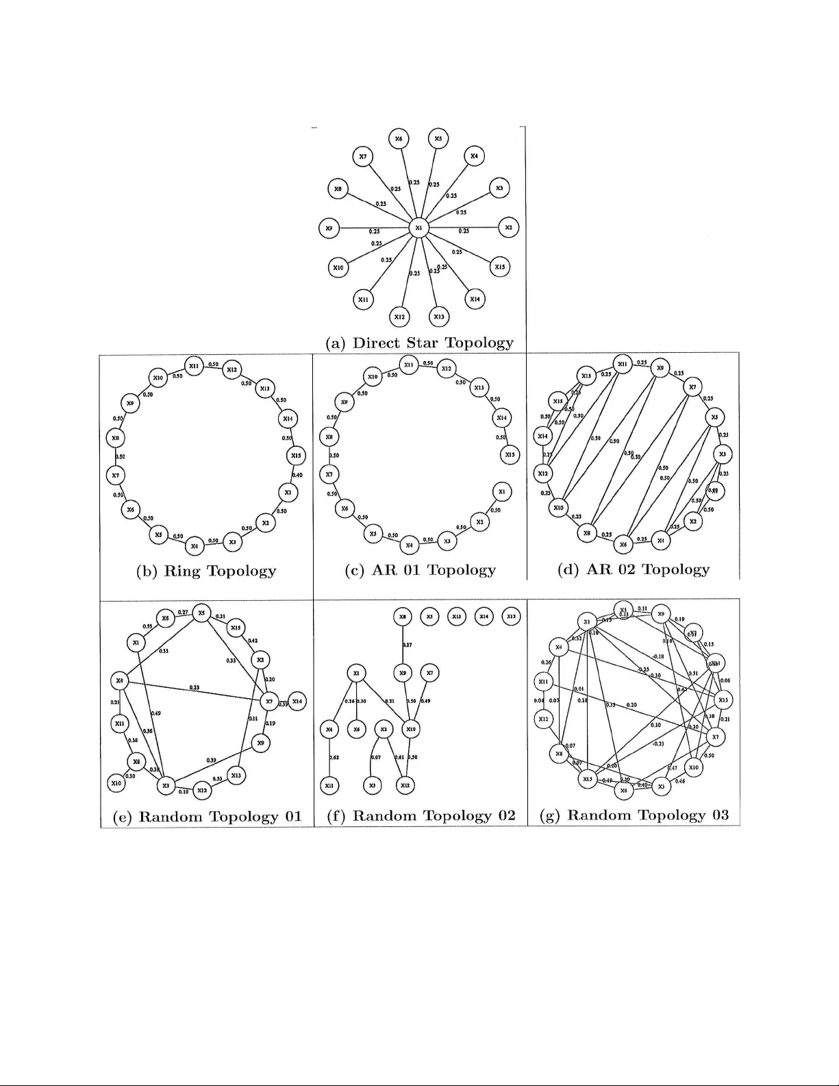
A path follo wing algorithm for Sparse Pseudo-Lik eliho o d In v erse Co v ariance Estimation (SPLICE) Guilherme V. Ro c ha, P eng Zhao, Bin Y u Octob er 22, 2018 Abstract Giv en n observ ations of a p -dimensional random v ector, the co v ariance matrix and its in v erse (precision matrix) are needed in a wide range of applications. Sample co v ariance (e.g. its eigenstructure) can misb eha v e when p is comparable to the sample size n . Regularization is often used to mitigate the problem. In this pap er, we prop osed an ` 1 p enalized pseudo-likelihoo d estimate for the inv erse cov ari- ance matrix. This estimate is sparse due to the ` 1 p enalt y , and w e term this metho d SPLICE. Its regularization path can b e computed via an algorithm based on the homotopy/LARS-Lasso algorithm. Simulation studies are carried out for v arious in verse co v ariance structures for p = 15 and n = 20 , 1000. W e compare SPLICE with the ` 1 p enalized likelihoo d estimate and a ` 1 p e- nalized Cholesky decomposition based metho d. SPLICE gives the b est o verall p erformance in terms of three metrics on the precision matrix and R OC curve for mo del selection. Moreo ver, our sim ulation results demonstrate that the SPLICE estimates are p ositiv e-definite for most of the regularization path ev en though the restriction is not enforced. Ac kno wledgmen ts The authors gratefully ac knowledge the supp ort of NSF gran t DMS-0605165, ARO gran t W911NF- 05-1-0104, NSFC (60628102), and a gran t from MSRA. B. Y u also thanks the Miller Research Professorship in Spring 2004 from the Miller Institute at Universit y of California at Berk eley and a 2006 Guggenheim F ellowship. G. Ro c ha also ackno wledges helpful comments by Ram Ra jagopal, Garv esh Raskutti, Pradeep Ravikumar and Vincent V u. 1 In tro duction Co v ariance matrices are p erhaps the simplest statistical measure of asso ciation b et ween a set of v ariables and widely used. Still, the estimation of cov ariance matrices is extremely data h ungry , as the num b er of fitted parameters gro ws rapidly with the num b er of observ ed v ariables p . Global prop erties of the estimated co v ariance matrix, such as its eigenstructure, are often used (e.g. Prin- cipal Comp onen t Analysis, Jolliffe, 2002). Such global parameters ma y fail to b e consisten tly estimated when the num b er of v ariables p is non-negligible in the comparison to the sample size n . As one example, it is a w ell-known fact that the eigenv alues and eigenv ectors of an estimated 1 co v ariance matrix are inconsisten t when the ratio p n do es not v anish asymptotically (Marchenk o and Pastur, 1967; Paul et al., 2008). Data sets with a large num ber of observed v ariables p and small n um b er of observ ations n are no w a common o ccurrence in statistics. Mo deling such data sets creates a need for regularization pro cedures capable of imp osing sensible structure on the estimated co v ariance matrix while b eing computationally efficient. Man y alternative approac hes exist for improving the properties of cov ariance matrix estimates. Shrinkage metho ds for cov ariance estimation w ere first considered in Stein (1975, 1986) as a w ay to correct the o verdispersion of the eigen v alues of estimates of large cov ariance matrices. Ledoit and W olf (2004) present a shrink age estimator that is the asymptotically optimal con vex linear com- bination of the sample cov ariance matrix and the identit y matrix with resp ect to the F ro eb enius norm. Daniels and Kass (1999, 2001) prop ose alternative strategies using shrink age tow ard diag- onal and more ge neral matrices. F actorial mo dels ha ve also b een used as a strategy to regularize estimates of co v ariance matrices (F an et al., 2006). T ap ering the cov ariance matrix is frequently used in time series and spatial mo dels and hav e b een used recen tly to improv e the p erformance of co v ariance matrix estimates used b y classifiers based on linear discriminan t analysis (Bick el and Levina, 2004) and in Kalman filter ensembles (F urrer and Bengtsson, 2007). Regularization of the co v ariance matrix can also b e ac hieved by r e gularizing its eigenve ctors (Johnstone and Lu, 2004; Zou et al., 2006). Covarianc e sele ction metho ds for estimating cov ariance matrices consist of imp osing sparsity on the precision matrix (i.e., the inv erse of the cov ariance matrix). The Sparse Pseudo-Lik eliho o d In verse Co v ariance Estimates (SPLICE) prop osed in this pap er fall into this category . This family of metho ds w as introduced by Dempster (1972). An adv an tage of imp osing structure on the precision matrix stems from its close connections to linear regression. F or instance, W u and Pourahmadi (2003) use, for a fixed order of the random vector, a parametrization of the precision matrix C in terms of a decomp osition C = U 0 DU with U upper-triangular with unit diagonal and D a diagonal matrix. The parameters U and D are then estimated through p linear regressions and Ak aik e’s Information Criterion (AIC, Ak aik e, 1973) is used to promote sparsity in U . A similar co v ariance selection metho d is presented in Bilmes (2000). More recen tly , Bick el and Levina (2008) ha ve obtained conditions ensuring consistency in the op erator norm (sp ectral norm) for precision matrix estimates based on banded Cholesky factors. Two disadv antages of imp osing the sparsit y in the factor U are: sparsity in U do es not necessarily translates into sparsity of C and; the sparsit y structure in U is sensitive to the order of the random v ariables within the random v ector. The SPLICE estimates prop osed in this pap er constitute an attempt at tac kling these issues. The AIC selection criterion used in W u and Pourahmadi (2003) requires, in its exact form, that the estimates b e computed for all subsets of the parameters in U . A more computationally tractable alternativ e for p erforming parameter selection consists in p enalizing parameter estimates b y their ` 1 -norm (Breiman, 1995; Tibshirani, 1996; Chen et al., 2001), p opularly known as the LASSO in the context of least squares linear regression. The computational adv an tage of the ` 1 - p enalization ov er p enalization by the dimension of the parameter b eing fitted ( ` 0 -norm) – suc h as in AIC – stems from its con vexit y (Boyd and V anden b erghe, 2004). Homotopy algorithms for tracing the en tire LASSO regularization path hav e recently b ecome a v ailable (Osb orne et al., 2000; Efron et al., 2004). Given the high-dimensionalit y of mo dern da ys data sets, it is no surprise that ` 1 -p enalization has found its wa y in to the cov ariance selection literature. Huang et al. (2006) propose a co v ariance selection estimate corresp onding to an ` 1 -p enalt y v ersion of the Cholesky estimate of W u and Pourahmadi (2003). The off-diagonal terms of U are 2 p enalized by their ` 1 -norm and cross-v alidation is used to select a suitable regularization param- eter. While this metho d is v ery computationally tractable (an algorithm based on the homotopy algorithm for linear regressions is detailed b elo w in App endix B.1), it still suffer from the deficien- cies of Cholesky-based metho ds. Alternativ ely , Banerjee et al. (2005), Banerjee et al. (2007), Y uan and Lin (2007), and F riedman et al. (2008) consider an estimate defined b y the Maximum Lik e- liho od of the precision matrix for the Gaussian case p enalized by the ` 1 -norm of its off-diagonal terms. While these metho ds imp ose sparsity directly in the precision matrix, no path-follo wing algorithms are currently av ailable for them. Rothman et al. (2007) analyze the prop erties of esti- mates defined in terms of ` 1 -p enalization of the exact Gaussian neg-loglik eliho o d and introduce a p erm utation inv ariant metho d based on the Cholesky decomp osition to av oid the computational cost of semi-definite programming. The SPLICE estimates presented here imp ose sparsit y constrain ts directly on the precision matrix. Moreo ver the entire regularization path of SPLICE estimates can b e computed by homotop y algorithms. It is based on previous work b y Meinshausen and B ¨ uhlmann (2006) for neigh b orho od selection in Gaussian graphical mo dels. While Meinshausen and B ¨ uhlmann (2006) use p separate linear regressions to estimate the neigh b orho od of one no de at a time, we prop ose merging all p linear regressions in to a single least squares problem where the observ ations asso ciated to each regression are weigh ted according to their conditional v ariances. The loss function th us formed can b e interpreted as a pseudo neg-loglikelihoo d (Besag, 1974) in the Gaussian case. T o this pseudo-negloglik eliho o d minimization, we add symmetry constrain ts and a w eighted v ersion of the ` 1 -p enalt y on off-diagonal terms to promote sparsity . The SPLICE estimate can b e in terpreted as an approximate solution following from replacing the exact neg-loglikelihoo d in Banerjee et al. (2007) b y a quadratic surrogate (the pseudo neg-loglikelihoo d). The main adv an tage of SPLICE estimates is algorithmic: by use of a prop er parametrization, the problem inv olv ed in tracing the SPLICE regularization path can b e recast as a linear regression problem and th us ame nable to b e solved by a homotopy algorithm as in Osb orne et al. (2000) and Efron et al. (2004). T o a void computationally exp ensiv e cross-v alidation, w e use information criteria to select a prop er amount of regularization. W e compare the use of Ak aik e’s Information criterion (AIC, Ak aik e, 1973), a small-sample corrected version of the AIC (AIC c , Hurvich et al., 1998) and the Bay esian Information Criterion (BIC, Sch w artz, 1978) for selecting the prop er amoun t of regularization. W e use simulations to compare SPLICE estimates to the ` 1 -p enalized maxim um likelihoo d estimates (Banerjee et al., 2005, 2007; Y uan and Lin, 2007; F riedman et al., 2008) and to the ` 1 -p enalized Cholesky approac h in Huang et al. (2006). W e hav e simulated b oth small and large sample data sets. Our simulations include mo del structures commonly used in the literature (ring and star top ologies, AR pro cesses) as w ell as a few randomly generated mo del structures. SPLICE had the b est p erformance in terms of the quadratic loss and the sp ectral norm of the precision matrix deviation ( k C − ˆ C k 2 ). It also p erformed well in terms of the entrop y loss. SPLICE had a remark ably go od performance in terms of selecting the off-diagonal terms of the precision matrix: in the comparison with Cholesky , SPLICE incurred a smaller n umber of false positives to select a given n umber of true p ositiv es; in the comparison with the p enalized exact maxim um lik elihoo d estimates, the path follo wing algorithm allows for a more careful exploration of the space of alternativ e mo dels. The remainder of this pap er is organized as follows. Section 2 presents our pseudo-likelihoo d surrogate function and some of its prop erties. Section 3 presents the homotopy algorithm used to trace the SPLICE regularization path. Section 4 presents simulation results comparing the 3 SPLICE estimates with some alternativ e regularized metho ds. Finally , Section 5 concludes with a short discussion. 2 An appro ximate loss function for in v erse cov ariance estimation In this section, w e establish a parametrization of the precision matrix Σ − 1 of a random vector X in terms of the co efficients in the linear regressions among its comp onen ts. W e emphasize that the parametrization w e use differs from the one previously used by W u and Pourahmadi (2003). Our alternativ e parametrization is used to extend the approac h used by Meinshausen and B ¨ uhlmann (2006) for the purp ose of estimation of sparse precision matrices. The resulting loss function can b e interpreted as a pseudo-likelihoo d function in the Gaussian case. F or non-Gaussian data, the minimizer of the empirical risk function based on the loss function we propose still yields consistent estimates. The loss function we prop ose also has close connections to linear regression and lends itself w ell for a homotop y algorithm in the spirit of Osb orne et al. (2000) and Efron et al. (2004). A comparison of this approximate loss function to its exact counterpart in the Gaus sian case suggests that the appro ximation is b etter the sparser the precision matrix. In what follows, X is a R n × p matrix containing in each of its n rows observ ations of the zero- mean random vector X with co v ariance matrix Σ. Denote by X j the j -th entry of X and b y X J ∗ the ( p − 1) dimensional v ector resulting from deleting X j from X . F or a given j , w e can p erm ute the order of the v ariables in X and partition Σ to get: co v  X j X J ∗  =  σ j,j Σ j,J ∗ Σ J ∗ ,j Σ J ∗ ,J ∗  where J ∗ corresp onds to the indices in X J ∗ , so σ j,j is a scalar, Σ j,J ∗ is a p − 1 dimensional row v ector and Σ J ∗ ,J ∗ is a ( p − 1) × ( p − 1) square matrix. Inv erting this partitioned matrix (see, for instance Ho c king, 1996) yield:  σ j,j Σ j,J ∗ Σ J ∗ ,j Σ J ∗ ,J ∗  − 1 = " 1 d 2 j − 1 d 2 j β j M 1 M − 1 2 # , (1) where: β j =  β j, 1 . . . , β j,j − 1 , β j,j +1 , . . . , β j,p  = − Σ j,J ∗ Σ − 1 J ∗ ,J ∗ ∈ R ( p − 1) , d j = r  σ j,j − Σ j,J ∗ Σ − 1 J ∗ ,J ∗ Σ J ∗ ,j  ∈ R + , M 2 = Σ J ∗ ,J ∗ − Σ J ∗ ,j σ − 1 j,j Σ j,J ∗ , M 1 = − M − 1 2 ·  Σ − 1 J ∗ ,J ∗ Σ J ∗ ,j  = − 1 d 2 j β 0 j , , (the second equality due to symmetry). W e will fo cus on the d j and β j parameters in what follo ws. The parameters β j and d 2 j corresp ond resp ectiv ely to the co efficients and the exp ected v alue of the squared residuals of the b est linear mo del of X j based on X J ∗ , irresp ectiv ely of the distribution of X . In what follo ws, we will let β j k denote the co efficien t corresp onding to X k in the linear mo del of X j based on X J ∗ . W e define: 4 • D : a p × p diagonal matrix with d j along its diagonal and, • B : a p × p matrix with zeros along its diagonal and off-diagonal terms giv en by β j k . Using (1) for j = 1 , . . . , p yields: Σ − 1 = D − 2 ( I p − B ) (2) Since Σ − 1 is symmetric, (2) implies that the follo wing constraints hold: d 2 k β j k = d 2 j β kj , for j, k = 1 , . . . , p. (3) Equation (2) sho ws that the sparsity pattern of Σ − 1 can b e inferred from sparsity in the regres- sion co efficien ts con tained in B . Meinshausen and B ¨ uhlmann (2006) exploit this fact to estimate the neigh b orhoo d of a Gaussian graphical mo del. They use the LASSO (Tibshirani, 1996) to obtain sparse estimates of β j : ˆ β j ( λ j ) = arg min b j ∈ R p − 1 k X j − X J ∗ b j k 2 + λ j k b j k 1 , for j = 1 , . . . , p (4) The neigh b orho od of the no de X j w as then estimated based on the entries of the ˆ β j that w ere set to zero. Minor inconsistencies could o ccur as the regressions are run separately . As an example, one could ha ve ˆ β j k ( λ j ) = 0 and ˆ β kj ( λ k ) 6 = 0, which Meinshausen and B ¨ uhlmann (2006) solv e by defining AND and OR rules for defining the estimated neighborho o d. T o extend the framework of Meinshausen and B ¨ uhlmann (2006) to the estimation of precision matrices the parameters d 2 j m ust also b e estimated and the symmetry constrain ts in (3) must b e enforced. W e use a pseudo-likelihoo d approach (Besag, 1974) to form a surrogate loss function in volving all terms of B and D . F or Gaussian X , the negative log-likelihoo d function of X j giv en X J ∗ is: log h p ( X j | X J ∗ , d 2 j , β j ) i = − n 2 log(2 π ) − n 2 log( d 2 j ) − 1 2  k X j − X J ∗ β j k 2 d 2 j  . (5) The parameters d 2 j and β j can b e consisten tly estimated by minimizing (5). A pseudo-neg- loglik eliho o d function can b e formed as: L ( X ; D , B ) = log  Q p j =1 p ( X j | X J ∗ , d 2 j , β j )  = − np 2 log(2 π ) − n 2 log det( D 2 ) − 1 2 tr  X ( I p − B 0 ) D − 2 ( I p − B ) X 0  . (6) An adv an tage of the surrogate L ( X ; D , B ) is that, for fixed D , it is a quadratic form in B . T o promote sparsit y on the precision matrix, we prop ose using a weigh ted ` 1 -p enalt y on B :  ˆ D ( λ ) , ˆ B ( λ )  = arg min ( B , D ) { n log det( D 2 ) + tr  X ( I p − B 0 ) D − 2 ( I p − B ) X 0  } + λ k B k w, 1 s.t.        b j j = 0 d 2 kk b j k = d 2 j j b kj d 2 kj = 0 , for k 6 = j d 2 j j ≥ 0 (7) 5 where k B k w, 1 = P p j,k =1 w j k | b j k | . F rom (2), the precision matrix estimate ˆ C ( λ ) is then giv en by: ˆ C ( λ ) = ˆ D − 2 ( λ ) h I p − ˆ B ( λ ) i . (8) The weigh ts w j k in (7) can b e adjusted to accommo date differences in scale b et ween the b j k parameters. In the remainder of this pap er, we fix w j k = 1 for all j, k such that j 6 = k (notice that the w eights w j j are irrelev an t since b j j = 0 for all j ). The main adv an tage of the pseudo-lik eliho od estimates as defined in (7) is algorithmic. Fixing D , the minimizer with resp ect to the B parameter is the solution of a ` 1 -p enalized least squares problem. Hence, for fixed D it is p ossible to adapt the homotop y/LARS-LASSO algorithm (Os- b orne et al., 2000; Efron et al., 2004) to obtain estimates for all v alues of λ . F or eac h fixed B , the minimizer with resp ect to D has a closed form solution. The algorithm presented in Section 3 is based on p erforming alternate optimization steps with resp ect to B and D to take adv an tage of these prop erties. One drawbac k of the precision matrix estimate ˆ C ( λ ) in (7) is that it cannot b e ensured to b e p ositiv e semi-definite. Ho w ever, from the optimality conditions to (7) it can b e prov en that for a large enough λ , all terms in the ˆ B ( λ ) matrix are set to zero. F or such highly regularized estimates, ˆ C ( λ ) is diagonal. Therefore, con tinuit y of the regularization path implies existence of λ ∗ < inf { λ : ˆ B ( λ ) = 0 } for whic h ˆ C ( λ ∗ ) is diagonal dominan t and thus p ositiv e semi-definite. W e return to the issue of positive semi-definiteness later in the pap er. W e will prov e in Section 2.4 that, when the ` 1 -norm is replaced by the ` 2 -norm, p ositiv e semi-definiteness is ensured for an y v alue of the regularization parameter. That suggests that a p enalt y similar to the elastic net (Zou and Hastie, 2005) can make the estimates along the ` 1 -norm regularization path p ositiv e semi-definite for a larger stretc h. In addition, in Section 4 w e present evidence that the ` 1 -norm p enalized estimates are p ositiv e semi-definite for most of the regularization path. 2.1 Alternativ e normalization Before w e mo ve on, we present a normalization of the X data matrix that leads to a more natural represen tation of the precision matrix ˆ C in terms of ˆ B and ˆ D while resulting in more conv enien t symmetry constrain ts. The symmetry constrain ts in (3) can b e rewritten in a more insightful form: d k d j β j k = d j d k β kj , for all j 6 = k . (9) This alternative representation, suggests that the symmetry constrain ts can b e more easily applied to a renormalized v ersion of the data. W e define: ˜ X = XD − 1 , and ˜ B = D − 1 BD . (10) Under this renormalization, ˜ B is symmetric, a fact that will b e explored in the algorithmic section b elo w to enforce the symmetry constraint within the homotopy algorithm used to trace regulariza- tion paths for SPLICE estimates. Another adv an tage of this renormalization is that the precision matrix estimate can b e written as: ˆ C ( λ ) = ˆ D − 1 h I p − ˆ ˜ B ( λ ) i ˆ D − 1 , (11) 6 making the analysis of the positive semi-definiteness of ˆ C ( λ ) easier: ˆ C ( λ ) is positive semi-definite if and only if I p − ˆ ˜ B ( λ ) is p ositiv e semi-definite. This condition is satisfied as long as the eigenv alues of ˆ ˜ B ( λ ) are smaller than 1. 2.2 Comparison of exact and pseudo-lik eliho o ds in the Gaussian case Banerjee et al. (2005), Y uan and Lin (2007), Banerjee et al. (2007) and F riedman et al. (2008) hav e considered estimates defined as the minimizers of the exact lik eliho o d p enalized by the ` 1 -norm of the off-diagonal terms of the precision matrix C : ˆ C exact ( λ ) = arg min C n log det( C ) + tr [ X CX 0 ] + λ k C k 1 s.t. C is symmetric p ositiv e semi-definite. (12) A comparison of the exact and pseudo-likelihoo d functions in terms of the ( D , ˜ B ) parametriza- tion suggests when the approximation will be appropriate. In terms of ( D , ˜ B ), the pseudo-likelihoo d function in (6) is: L ( X ; D , B ) = − np 2 log(2 π ) − n 2 log det( D 2 ) − 1 2 tr h ˜ X ( I p − ˜ B ) 2 ˜ X 0 i . (13) In the same parametrization, the exact lik eliho od function is: L exact ( X ; D , B ) = − np 2 log(2 π ) − n 2 log det h I p − ˜ B i − n 2 log det( D 2 ) − 1 2 tr h ˜ X  I p − ˜ B  ˜ X 0 i (14) A comparison b etw een (13) and (14) reveals tw o differences in the exact and pseudo neg-loglik eliho o d functions. First, the exact expression in v olv es one additional log det h I p − ˜ B i term not app earing in the surrogate expression. Secondly , in the squared deviation term, the surrogate expression has the weigh ting matrix h I p − ˜ B i squared in the comparison to the exact lik eliho o d. F or ˜ B = 0 , the log det v anishes and the weigh ting term equals identit y and th us idemp oten t. Since these t wo functions are contin uous in ˜ B , we can exp ect this approximation to work b etter the smaller the off-diagonal terms in ˜ B . In particular, in the completely sparse case, the tw o functions coincide and the appro ximation is exact. 2.3 Properties of the pseudo-lik eliho o d estimate In the classical setting where p is fixed and n grows to infinity , the unregularized pseudo-likelihoo d estimate ˆ C (0) is clearly consistent. The unconstrained estimates for β j and d 2 j are all consisten t. In adition, the symmetry constraints we imp ose are observed in the p opulation version and thus in tro duce no asymptotic bias in the (symmetry) constrained estimates. That in conjunction with the results from Knight and F u (2000) can b e used to pro ve that, as long as λ = o p ( n ) the ` 1 - p enalized estimates in (7) are consistent. Still in the classical setting, Y uan and Lin (2007) point out that the unp enalized estimate ˆ C (0) is not efficien t as it do es not coincide with the maxim um likelihoo d estimate. Ho wev er, the comparison of the exact and pseudo-likelihoo ds presented in Section 2.2 suggests that the loss in efficiency should be smaller the sparser the true precision matrix. In addition, the penalized pseudo- lik eliho o d estimate lends itself b etter for path following algorithms and can b e used to select an 7 appropriate λ while sim ultaneously providing a go o d starting p oin t for algorithms computing the exact solution. One interesting question we will not pursue in this pap er concerns the quality of the pseudo- lik eliho o d approximation in the non-classical setting where p n is allow ed to grow with n . In that case, the classical efficiency argumen t fa voring the exact maximum likelihoo d o v er the pseudo- lik eliho o d approximation no longer holds. T o the b est of our kno wledge, it is an op en question whether the penalized exact ML has adv an tages ov er a pseudo-lik eliho o d appro ximation in the non-parametric case ( p n gro wing with n ). 2.4 P enalization by ` 2 -norm and P ositive Semi-definiteness As mentioned abov e,the algorithm we propose in Section 3 suffers from the drawbac k of not enforc- ing a p ositiv e semi-definite constraint. Imp osing such constraint is costly in computational terms and would slow down our path following algorithm. As we will see in the exp erimen tal Section 4 b elo w, the unconstrained estimate is p ositive semi-definite for the greater part of the regularization path ev en in nearly singular designs. Before we review such exp erimen tal evidence, how ev er, we study an alternative p enalization that do es result in p ositiv e semi-definite estimates for all levels of regularization. Consider the p enalized pseudo-likelihoo d estimate defined b y: ˆ ˜ B 2 ( λ 2 ) = arg min ˜ B n tr h ( I p − ˜ B ) ˜ X 0 ˜ X ( I p − ˜ B 0 ) i + λ 2 · tr h ˜ B 0 ˜ B io s.t.  b j j = 0 ˜ b j k = ˜ b kj (15) Our next result establishes that the estimate defined by is p ositiv e semi-definite along its entire path: Theorem 1. L et ˆ C ( λ 2 ) = ˆ D 2 ( λ 2 ) − 1  I p − ˆ ˜ B 2 ( λ 2 )  ˆ D 2 ( λ 2 ) − 1 b e the pr e cision matrix estimate r e- sulting fr om (15). F or any ˆ D 2 ( λ 2 ) and λ 2 > 0 , the pr e cision matrix estimate ˆ C 2 ( λ 2 ) is p ositive semi-definite. This result suggests that the ` 2 -p enalt y may b e useful in inducing p ositiv e semi-definiteness. So an estimate incorp orating b oth ` 2 - and ` 1 -p enalties, ˆ ˜ B E N ( λ 2 , λ 1 ) = arg min ˜ B  tr h ( I p − ˜ B ) ˜ X 0 ˜ X ( I p − ˜ B 0 ) i + λ 2 · tr h ˜ B 0 ˜ B i + λ 1 ·    ˜ B 0 ˜ B    w, 1  s.t.  b j j = 0 ˜ b j k = ˜ b kj , (16) can hav e improv ed p erformance, ov er the ` 1 -p enalt y alone, in terms of p ositiv e semi-definiteness. The subscript E N is a reference to the Elastic Net penalty of Zou and Hastie (2005). In our exp erimen tal section b elo w (Section 4), w e hav e came across non-p ositive semi-definite precision matrix estimate in none other than a few replications. W e hence left a detailed study of the Elastic Net precision matrix estimate defined in (16) for future research. 8 3 Algorithms W e now detail an iterativ e algorithm for computing the regularization path for SPLICE estimates. The computational adv an tage of that approximate loss function used in (7) follows from tw o facts: • F or a fixed D , the optimization problem reduces to that of tracing a constrained LASSO path; • F or a fixed B , the optimizer ˆ D has a closed form solution; Based on these tw o facts, we prop ose an iterative algorithm for obtaining estimates ˆ D ( ˆ λ ) and ˆ B ( ˆ λ ). Within each step, the path for ˆ D and ˆ B as a function of the regularization parameter λ is traced and the choice of the regularization parameter λ is up dated. W e now describ e the steps of our SPLICE algorithm. 1. Let k = 1 and ˆ D 0 = diag  k X j k 2 2 n  p j =1 . 2. Rep eat until c onver genc e : (a) Set ˜ X = X ˆ D − 1 k − 1 and use a path-tracing algorithm for the regularized problem: ˆ ˜ B ( λ ) = arg min B n tr h ˜ X ( I − ˜ B 0 )( I − ˜ B ) ˜ X 0 i + λ · k ˜ B k ˜ w, 1 o s.t. ˜ b j k = ˜ b kj ˜ b j j = 0 (b) Compute the corresp onding path for D : ˆ D k ( λ ) = diag   k  I p − ˆ B ( λ )  X j k 2 2 n   p j =1 (c) Select a v alue for the regularization parameter ˆ λ k ; (d) Set ˆ B k = ˆ B ( ˆ λ k ) and ˆ D k = ˆ D ( ˆ λ k ); 3. Return the estimate ˆ C = ˆ D − 1 k ( I − ˆ ˜ B k ) ˆ D − 1 k ; A subtle but imp ortan t detail is the weigh ting vector ˜ w used when applying the p enalt y in step 2.(a). Since the path is traced in terms of the normalized ˜ B parameter instead of B , a correction m ust b e made in these w eights. This can b e determined b y noticing that: k B k w, 1 = p X j,k =1 w j k | b j k | = p X j,k =1 w j k d j d k     d k d j b j k     = p X j,k =1 ˜ w j k    ˜ b j k    = k ˜ B k ˜ w, 1 , as long as ˜ w j k = w j k d j d k . As mentioned b efore, we fix w j k = 1 throughout this pap er, so w e set ˜ w j k = w j k d j d k in our exp eriments. Of course, d j are unknown so the current estimate is plugged-in ev ery time step 2.(a) is executed. In the remainder of this section, we sho w how to adapt the homotopy/LARS-LASSO algorithm to enforce the symmetry constraints d 2 k b j k = d 2 j b kj along the regularization path, how to select ˆ B and ˆ D from the path, and discuss some conv ergence issues related to the algorithm ab ov e. 9 3.1 Enforcing the symmetry constraints along the path The expression defining the regularization path in step 2.(a) of the SPLICE algorithm ab o v e can b e rewritten as: ˆ B ( λ ) = arg min B v ec  ˜ X ( I p − B 0 )  0 v ec  ˜ X ( I p − B 0 )  + λ k B k w, 1 s.t. b j j = 0 b j k = b kj , (17) whic h is a quadratic form in B p enalized b y a w eighted version of its ` 1 -norm. T o enforce the equalit y restriction in (17), we massage the data into an appropriate form so the homotopy/LARS- LASSO algorithm can b e used in its original form. The optimization problem in (17) corresp onds to a constrained version of a p enalized regression of mo dified resp onse ( Y ) and predictors ( Z ) given by: Y =      ˜ X 1 ˜ X 2 . . . ˜ X p      and Z =        ˜ X 1 ∗ 0 0 · · · 0 0 ˜ X 2 ∗ 0 · · · 0 0 0 ˜ X 3 ∗ · · · 0 . . . . . . . . . . . . . . . 0 0 0 · · · ˜ X p ∗        Since the “mo del” for Y giv en Z is additiv e, w e can force b j k = b j k b y creating a mo dified design matrix ˜ Z where the columns corresp onding to b j k and b kj are summed in to a single column. More precisely , the column corresp onding to ˜ b j k with j < k in the ˜ Z design matrix has all elements set to zero except for the rows corresp onding to X k and X j in the Y vector. These ro ws m ust b e set to ˜ X j and ˜ X k resp ectiv ely: ˜ Z =          ˜ X 2 ˜ X 3 · · · ˜ X p − 1 ˜ X p 0 · · · 0 · · · 0 ˜ X 1 0 · · · 0 0 ˜ X 3 · · · ˜ X p · · · 0 0 ˜ X 1 · · · 0 0 ˜ X 2 · · · 0 · · · 0 . . . 0 0 · · · ˜ X 1 0 · · · 0 0 · · · ˜ X p 0 0 · · · 0 ˜ X 1 · · · 0 0 · · · ˜ X p − 1          The path for the constrained ˜ B ( λ ) can then b e traced by simply applying a weigh ted version of the LASSO algorithm to Y and ˜ Z . W e emphasize that, even though the design matrix ˜ Z has O ( np 3 ) elements, it is extremely sparse. It can b e prov ed that it contains only O ( np 2 ) non-zero terms. It is thus crucial that the implemen tation of the homotop y/LARS-LASSO algorithm used to trace this path mak e use of the sparsity of the design matrix. 10 3.2 Computational complexity of one step of the algorithm The algorithm prop osed ab o ve to trace the regularization path of ˆ ˜ B ( λ ) uses the homotop y/LARS- LASSO algorithm with a mo dified regression with p ( p − 1) 2 regressors and np observ ations. The computational complexit y of the k -th step of the homotop y algorithm in step 2.(a) is of order O ( a 2 k + a k np ), where a k denotes the num b er of non-zero terms on the upp er triangular, off-diagonal of ˜ B ( λ k ) (a detailed analysis is presented in Efron et al., 2004). Clearly , the computational cost increases rapidly as more off-diagonal terms are added to the precision matrix. When p grows with n keeping a constant ratio p/n , we find it plausible that most selection criteria will pick estimates at the most regularized regions of the path: a data sample can only supp ort so man y degrees of freedom. Th us, incorp orating early stopping criteria in to the path tracing at step 2.(a) of the SPLICE algorithm can greatly reduce the computational cost of obtaining the path ev en further without degrading the statistical p erformance of the resulting estimates. If one insists in having the entire precision matrix path, the SPLICE algorithm is still p olynomial in p and n . In the case where no v ariables are dropped and the v ariables are added one at a time, the complexit y of the first K steps of the path is given b y O ( K 3 + K 2 np ). Under the same assumptions and setting K = 0 . 5 · p ( p − 1), the SPLICE algorithm has cost of order O ( p 6 + np 5 ) to compute the en tire path of solutions to the pseudo-lik eliho o d problem. As a comparison, an algorithm presen ted b y Banerjee et al. (2005) has a cost of order O ( p 4 . 5 η ) to compute an approximate solution for the p enalized exact likelihoo d at a single point of the path, where η represents the desired level of appro ximation. 3.3 Selection criteria for λ : Differen t criteria can b e used to pick a pair B , D from the regularization path (cf. 2(c) in the SPLICE algorithm). In the exp erimen t section b elo w, we show the results of using Ak aik e’s In- formation Criterion (AIC, Ak aik e, 1973), the Bay esian information Criterion (BIC, Sch w artz, 1978) and a corrected version of the AIC criterion (AIC c , Hurvich et al., 1998) using the un biased estimate of the degrees of freedom of the LASSO along the regularization path. More precisely , we set: ˆ λ = arg min λ L exact ( X , ˆ D , ˆ B ( λ )) + K ( n, b df( ˆ C ( λ )) where: K ( n, b df( ˆ C ( λ ))) =            2 b df( ˆ C ( λ )) , for AIC , 1+ c df ( ˆ C ( λ )) n 1 − c df ( ˆ C ( λ ))+2 n , for AIC c , log( n ) b df( ˆ C ( λ )) , for BIC , As our estimate of the degrees of freedom along the path, we follow Zou et al. (2007) and use p plus the n umber of non-zero terms in the upp er triangular section of ˆ B ( λ ), that is, b df( λ ) = p +    n ( i, j ) : i < j and ˆ B ij ( λ ) 6 = 0 o    . (18) The p term in expression (18) stems from the degrees of freedom used for estimating the means. 11 3.4 Stopping criterion W e now determine the conv ergence criterion we used to finish the lo op started in step (2) of the SPLICE algorithm. T o do that, w e lo ok at the v ariation in the terms of the diagonal matrix D . W e stop the algorithm once: max 1 ≤ j ≤ p ( log [ ˆ D k +1 ] j [ ˆ D k ] j !) < 10 − 2 , or when the n umber of iterations exceeds a fixed n umber Q , whichev er o ccurs first. W e hav e also observ ed that letting λ k +1 differ from λ k often resulted in oscillating estimates caused solely by small v ariations in λ from one step to the next. T o a void this issue, we fixed the regularization parameter λ after a n umber M < Q of “warm-up” rounds. W e ha ve set M = 6 and Q = 100 for the sim ulations in Section 4. F or most cases, the selected v alue of λ and the ˆ D matrix had b ecome stable and the algorithm had con verged b efore either the maxim um num b er M of “warm-up” steps was reac hed. 4 Numerical Results In this section, we compare the results obtained b y SPLICE in terms of estimation accuracy and mo del selection p erformance to other co v ariance selection methods, namely the Cholesky co v ariance selection pro cedure prop osed by Huang et al. (2006) (Cholesky) and the ` 1 -p enalized maximum lik eliho o d estimate studied previously b y Y uan and Lin (2007); Banerjee et al. (2005) and F riedman et al. (2008) (Exact PML). W e compare the effectiveness of three different selection criteria – AIC, AIC c and BIC (see Section 3.3)– in picking an estimate from the SPLICE, Cholesky and Penalized Exact Log-Lik eliho o d regularization paths. W e also compare the mo del selection p erformance o ver the en tire regularization path using ROC curves (for details, see 4.1.2). Finally , we study the p ositiv e semi-definiteness of the SPLICE estimates along the regularization path in a near-singular design. 4.1 Comparison of SPLICE to alternativ e metho ds Figure 1 shows the graphical mo dels corresp onding to the sim ulated data sets we will b e using to compare SPLICE, Cholesky and Exact PML in terms of estimation accuracy and cov ariance selection. All designs inv olv e a 15-dimensional zero-mean Gaussian random vector ( p = 15) with precision matrix implied b y the graphical mo dels shown in Figure 1. A relatively small sample size is used to emulate the effect of high-dimensionality . F or all comparisons, the estimates are computed based on either 20 or 1,000 indep endent samples from eac h distribution (small sample case: n = 20, large sample case: n = 1 , 000). The results presented here are based on r = 200 replications for eac h case. Before w e show the results, a few words on our choice of simulation cases: • The star mo del (see Figure 1 panel a) pro vides an in teresting example where the ordering of the v ariables can hav e a great influence in the results of an order-dep enden t metho d suc h as Cholesky . In the Dir e ct Star case, the h ub v ariable is the first en try in the 15-dimensional random vector (as shown in the figure). Conditioning on the first v ariable ( X 1 ) makes all other v ariables indep enden t ( X 2 , . . . , X 15 ). Mean while, in the inverte d star top ology , the hub 12 Figure 1: Simulated cases: In this table, the top ology of the precision matrix for all simulated cases is shown. In eac h case, the precision matrix is normalized to ha ve unit diagonal. The edges sho w the v alue of c ij whenev er it differs from zero. 13 v ariable is put at the last position of the 15-dimensional random v ector. As a result, no conditional indep endence is present until the last v ariable is added to the conditioning set. • In the “AR-like” family of mo dels (see Figure 1 panels b, c and d) each 15-dimensional random v ector corresp onds (panels c and d) or is very similar (panel b) to 15 observ ations from an auto-regressiv e pro cess. This family of mo dels tends to giv e some adv an tage to the Cholesky pro cedure as the ordering of the v ariables within the vector con tain some information ab out the dependency structure among the v ariables. The cases in this family are lo osely based on some of the sim ulation designs used in Y uan and Lin (2007); • The “random” designs (see Figure 1 panels e, f and g) were obtained by randomly choosing precision matrices as described in App endix C. W e used these designs to mak e sure our results are v alid in somewhat less structured environmen ts. 4.1.1 Estimation accuracy of SPLICE, Cholesky and Exact PML W e ev aluate the accuracy of the precision matrix estimates according to following four metrics. • The quadratic loss of the estimated precision matrix, defined as ∆ 2 ( C , ˆ C ) = tr  C ˆ C − 1 − I p  2 . • The en tropy loss at the estimated precision matrix, defined as ∆ e ( C , ˆ C ) = tr  C ˆ C − 1  − log  C ˆ C − 1  − n. • The sp ectral norm of the deviation of the estimated precision matrix  ˆ C − C  where the sp ectral norm of a square matrix A is defined as k A k 2 = sup x k x 0 A x k 2 k x k 2 . • The sp ectral norm of the deviation of the estimated cov ariance matrix  ˆ Σ − Σ  . F or each of Cholesky , SPLICE and Exact PML, we compute estimates taken from their paths using the selection criteria men tioned in 3.3: AIC, AIC c and BIC. The Cholesky and SPLICE estimates are c hosen from the breakp oints of their resp ectiv e regularization paths. The path trac- ing algorithm w e ha v e used for the Cholesky estimate is sketc hed in Appendix B.1. The path follo wing algorithm for SPLICE is the one describ ed in Section 3. The Exact ML estimate is cho- sen by minimizing the selection criterion ov er an equally spaced 500-p oin t λ -grid b et ween 0 and the maximum absolute v alue of the off-diagonal terms of the sample co v ariance matrix. W e used the implementation of the ` 1 -p enalized Exact log-likelihoo d for Matlab made av ailable at Prof. Alexandre D’Aspremon t’s web site ( http://www.princeton.edu/ ∼ aspremon/ ). Bo xplots of the different accuracy measures for each of the metho ds and selection criteria are sho wn in Figures 2, 3 and 4 for the small sample case ( n = 20), and in Figures 5, 6 and 7 for the large sample case ( n = 1 , 000). F or larger sample sizes, the Cholesky estimates do suffer some deterioration in terms of the en tropy and quadratic losses when an inappropriate ordering of the v ariables is used. As we will later see, an inappropriate ordering can also degrade the Cholesky p erformance in terms of selecting the right cov ariance terms. A comparison of the differen t metho ds reveals that the b est metho d to use dep ends on whether the metric used is on the in verse cov ariance (precision matrix) or cov ariance matrix. 14 P erformance Metric Recommended pro cedure ∆ 2 ( C , ˆ C ) SPLICE + AIC ∆ e ( C , ˆ C ) SPLICE + AIC k ˆ C − C k 2 SPLICE + AIC c (for smaller sample size, n = 20) SPLICE + BIC (for larger sample size, n = 1 , 000) k ˆ Σ − Σ k 2 Exact p enalized ML + AIC T able 1: Suitable estimation methods for different cov ariance structures and p erfor- mance metrics: The results sho wn here are a summary of the results shown in Figures 2 through 7. F or eac h metric, w e sho w the b est combination of estimation metho d and selection criterion based on our sim ulations. • With resp ect to all the three metrics on the in verse co v ariance (quadratic, en tropy and sp ectral norm losses), the best results are achiev ed by SPLICE. In the case of the quadratic loss, this result can b e partially attributed to the similarit y b et ween the quadratic loss and the pseudo-lik eliho o d function used in the SPLICE estimate. In terms of the sp ectral norm on the precision matrix ( k C − ˆ C k 2 ), SPLICE p erformed particularly w ell in larger sample sizes ( n = 1 , 000). F or the quadratic and entrop y loss functions, AIC was the criterion pic king the b est SPLICE estimates. In terms of the sp ectral norm loss, SPLICE p erforms b etter when coupled with AIC c for small sample sizes ( n = 20) and when coupled with BIC in larger sample sizes ( n = 1 , 000). • In terms of the spectral norm of the co v ariance estimate deviation ( k Σ − ˆ Σ k 2 ), the b est p erformance was ac hieved b y Exact PML. The p erformance of Exact PML w as somewhat insensitiv e to the selection criterion used in many cases: this may b e caused by the uniform grid on λ missing regions where the p enalized mo dels rapidly change as λ v aries. Based on the cases where the selection criterion affected the p erformance of Exact PML, BIC seems to yield the b est results in terms of k Σ − ˆ Σ k 2 . F or ease of reference, these results are collected in T able 1. 4.1.2 Mo del Selection p erformance of SPLICE T o ev aluate the mo del selection p erformance of the different co v ariance selection metho ds, w e compare their Relative Op erating Characteristic (ROC) curves defined as a curve con taining in 15 Figure 2: Accuracy metrics for precision matrix estimates in the Star cases for p = 15 and n = 20 16 Figure 3: Accuracy metrics for precision matrix estimates in the AR-lik e cases for p = 15 and n = 20 17 Figure 4: Accuracy metrics for precision matrix estimates in the randomly generated designs for p = 15 and n = 20 18 Figure 5: Accuracy metrics for precision matrix estimates in the Star cases for p = 15 and n = 1 , 000 : 19 Figure 6: Accuracy metrics for precision matrix estimates in the AR-lik e cases for p = 15 and n = 1 , 000 20 Figure 7: Accuracy metrics for precision matrix estimates in the randomly generated designs for p = 15 and n = 1 , 000 21 its horizontal axis the minimal num ber of false p ositiv es that is incurred on av erage for a giv en n umber of true n umber of p ositiv es, shown on the vertical axis, to be identified. The R OC curve for a metho d shows its mo del selection p erformance ov er all p ossible choices of the tuning parameter λ . W e hav e c hosen to compare ROC curv es instead of the results for particular selection criterion as differen t applications may p enalize false p ositiv es and negativ es differently . F or a fixed num b er of true p ositiv es on the vertical axis, we wan t the exp ected minimal n umber of false p ositives to b e as low as p ossible. A co v ariance selection metho d is thus b etter the closer its R OC curve is to the upp er left side of the plot. Figures 8 and 9 compare the ROC curv es for the Cholesky and SPLICE cov ariance selection pro cedures for sample sizes n = 20 and n = 1 , 000 resp ectiv ely . The Exact ML do es not ha v e its ROC curve shown: the grid used to appro ximate its regularization path often did not include estimates with a sp ecific num b er of true p ositives. A finer grid can ameliorate the problem, but w ould b e prohibitively exp ensiv e to compute (recall we used a grid with 500 equally spaced v alues of λ ). This illustrates an adv an tage of path follo wing algorithms ov er using grids: path follo wing p erforms a more thorough search on the space of mo dels. The mean ROC curv es on Figures 8 and 9 sho w that SPLICE had a b etter p erformance in terms of mo del selection in comparison to the Cholesky metho d ov er all cases considered. In addition, for a given num b er of true p ositives, the n umber of false p ositiv es incurred b y SPLICE decreases significan tly as the sample size increases. Our results also suggest that, with the exception of the Random Design 02, the chance that the SPLICE path contains the true mo del approaches one as the sample size increases for all sim ulated cases. Finally , we consider the effect of ordering the v ariables on the selection p erformance of SPLICE and Cholesky . T o do this, w e restrict atten tion to the “star” cases and compare the p erformance of SPLICE and Cholesky when the v ariables are presen ted in the “correct” order ( X 1 , X 2 , . . . , X p ) and in the in verted order ( X p , X p − 1 , . . . , X 1 ). Figure 10 shows the b oxplot of the minimal n umber of false p ositiv es on 200 replications of the Cholesky and SPLICE paths for selected n umber of true p ositiv es in the small sample case ( n = 20). In addition to outp erforming Cholesky b y a wide margin, SPLICE is not sensitive to the order in which the v ariables are presented. Cholesky , on the other hand, suffers some further degradation in terms of mo del selection when the v ariables are presen ted in the reverse order. 4.2 P ositiv e Semi-Definiteness along the regularization path As noted in Section 2 ab o ve, there is no theoretical guarantee that the SPLICE estimates b e p ositiv e semi-definite. In the somewhat well-behav ed cases studied in the exp erimen ts of Section 4.1 (see Figure 1) all of the estimates selected by either AIC c and BIC were p ositiv e semi-definite cases. In only 6 out of the 1,600 sim ulated cases, did AIC c ho ose a sligh tly negative SPLICE estimate. This, how ev er, tells little ab out the p ositive-definiteness of SPLICE estimates in badly b ehav ed cases. W e now pro vide some exp erimen tal evidence that the SPLICE estimates can b e p ositiv e semi-definite for most of the regularization path ev en when the true cov ariance matrix is nearly singular. The results rep orted for this exp erimen t are based on 200 replications of SPLICE applied to a data matrix X sampled from a Gaussian distribution with near singular cov ariance matrix. The num b er of observ ations ( n = 40) and the dimension of the problem ( p = 30) are kept fixed throughout. T o obtain a v ariet y of near singular cov ariance matrices, the sample co v ariance Σ ∈ 22 Figure 8: “Mean R OC curves” for the Cholesky and SPLICE co v ariance selection for p = 15 and n = 20 : Within eac h panel, the relative op erating characteristic (ROC) curv e shows the mean minimal num b er of false p ositiv es (horizontal axis) needed to ac hieve a given n umber of true p ositiv es (vertical axis) for b oth the SPLICE (solid lines) and Cholesky (dashed lines). A selection pro cedure is b etter the more its curve approac hes the upp er left corner of the plot. Our results suggest that SPLICE trades off b etter than Cholesky b et ween false and true p ositiv es across all cases considered. 23 Figure 9: “Mean ROC curves” for the Cholesky and SPLICE co v ariance selection for p = 15 and n = 1 , 000 : Within eac h panel, the relative op erating characteristic (ROC) curv e shows the mean minimal num b er of false p ositiv es (horizontal axis) needed to ac hieve a given n umber of true p ositiv es (vertical axis) for b oth the SPLICE (solid lines) and Cholesky (dashed lines). A selection pro cedure is b etter the more its curve approac hes the upp er left corner of the plot. Our results suggest that SPLICE pic ks correct cov ariance terms with a larger sample size for large enough sample sizes. The Cholesky estimates, how ev er, do not seem m uch more likely to select correct cov ariance terms in this larger sample size in the comparison with the case n = 20. 24 Figure 10: Horizon tal detail for ROC curv es in the “star” cases: Within each panel, we show a b oxplot of the minimal n umber of false p ositives on the path for the indicated num b er of true p ositiv es. Each panel can b e thought of as the b o xplot corresp onding to a horizon tal lay er on the graph shown in Figure 8. SPLICE is insensitiv e to the p erm utation of the v ariables (compate inv erted and direct). Cholesky p erforms worse than SPLICE in b oth the direct and in verted cases: its p erformance deteriorates further if the v ariables are presented in inv erted order. 25 R p × p of eac h of the 200 replications is sampled from: Σ ∼ Wishart( n, ¯ Σ) , with [ ¯ Σ] ij = 0 . 99 | i − j | . The cov ariance matrices sampled from distribution hav e exp ected v alue ¯ Σ, whic h is itself close to singular. W e let the num ber of degrees of freedom of the Wishart distribution b e small (equal to the sample size n = 30) to make designs close to singular more likely to happ en. Once Σ is sampled, the data matrix X is then formed from an i.i.d. sample of a N (0 , Σ) distribution. T o align the results along the path of differen t replications, we create an index ¯ λ formed by dividing a λ on the path by the the maximum λ at that path. This index v aries o v er [0 , 1] and lo wer v alues of ¯ λ corresp ond to less regularized estimate s. Figure 11 shows the minim um eigenv alue of ˆ C ( λ ) v ersus the index ¯ λ for the 200 simulated replications. W e can see that non-p ositiv e estimates only o ccur near the very end of the path (small v alues of λ ) even in suc h an extreme design. 5 Discussion In this pap er, we hav e defined Sparse Pseudo-Lik eliho o d Inv erse Cov ariance Estimates (SPLICEs) as a ` 1 -p enalized pseudo-likelihoo d estimate for precision matrices. The SPLICE loss function (6) is obtained from extending previous work by Meinshausen and B ¨ uhlmann (2006) to obtain estimates of precision matrix that are symmetric. The SPLICE estimates are formed from estimates of the co efficien ts and v ariance of the residuals of linear regression mo dels. The main adv an tage of the estimates prop osed here is algorithmic. The regularization path for SPLICE estimates can b e efficiently computed by alternating the estimation of co efficien ts and v ariance of the residuals of linear regressions. F or fixed estimates of the v ariance of residuals, the complete path of the regression co efficien ts can be traced efficiently using an adaptation of the homotop y/LARS-LASSO algorithm (Osb orne et al., 2000; Efron et al., 2004) that enforces the symmetry constraints along the path. Giv en the path of regression co efficients, the v ariance of the residuals can b e estimated by means of closed form solutions. An analysis of the complexity of the algorithm suggests that early stopping can reduce its computational cost further. A comparison of the pseudo-likelihoo d approximation to the exact lik eliho o d function pro vides another argument in fav or of early stopping: the pseudo-lik eliho o d approximation is b etter the sparser the estimated mo del. Th us moving on to the lesser sparse stretches of the regularization path can b e not only computationally costly but also coun terpro ductiv e to the quality of the estimates. W e hav e compared SPLICE with ` 1 -p enalized co v ariance estimates based on Cholesky decom- p osition (Huang et al., 2006) and the exact likelihoo d expression (Banerjee et al., 2005, 2007; Y uan and Lin, 2007; F riedman et al., 2008) for a v ariet y of sparse precision matrix cases and in terms of four different metrics, namely: quadratic loss, entrop y loss, sp ectral norm of C − ˆ C and sp ectral norm of Σ − ˆ Σ. SPLICE estimates had the b est p erformance in all metrics with the exception of the sp ectral norm of Σ − ˆ Σ. F or this last metric, the b est results were achiev ed by using the ` 1 -p enalized exact likelihoo d. In terms of selecting the righ t terms of the precision matrix, SPLICE was able to pick a given n umber of correct co v ariance terms while incurring in less false p ositiv es than the ` 1 -p enalized Cholesky estimates of Huang et al. (2006) in v arious simulated cases. Using an uniform grid for the exact p enalized maxim um likelihoo d provided few estimates with a mid-range n umber of correctly pick ed cov ariance terms. This reveals that path following metho ds p erform a more 26 Figure 11: Positiv e definiteness along SPLICE path: A t different vertical and horizontal scales, the tw o panels sho w the the minimum eigenv alue of the SPLICE estimate ˆ C ( λ ) along the regularization path as a function of the normalized regularization parameter ¯ λ . A t the unregularized extreme (small ¯ λ ), ˆ C can ha ve v ery negativ e eigen v alues (left panel). Ho wev er, for a long stretc h of the regularization path – o ver 90% of the path as measured b y the index λ – the SPLICE estimate ˆ C is p ositiv e definite (righ t panel). 27 thorough exploration of the mo del space than p enalized estimates computed on (pre-determined) grids of v alues for the regularization parameter. While SPLICE estimates are not guaran teed to b e p ositiv e semi-definite along the en tire regu- larization path, they ha ve b een observed to be such for most of the path even in a almost singular problem. Over tamer cases, the estimates selected by AIC, BIC and AIC c w ere positive semi- definite in the o verwhelming ma jorit y of cases (1,594 out of 1,600). A Pro ofs A.1 P ositiv e Semi-definiteness of ` 2 -p enalized Pseudo-likelihoo d estimate W e no w prov e Theorem 1. First, we rewrite the ` 2 -norm p enalt y in a more con venien t form: p + tr h ˜ B 0 ˜ B i = p + p X j =1 p X k =1 ( − b j k ) 2 = p X j =1 (1 − b j j ) 2 + p X j =1 p X k =1 ( − b j k ) 2 = tr h ( I p − ˜ B ) 0 ( I p − ˜ B ) i Hence, the ` 2 -p enalized estimate defined in (15), can b e rewritten as: ˆ ˜ B 2 ( λ 2 ) = arg min ˜ B tr h ( I p − ˜ B )  ˜ X 0 ˜ X + λ 2 I p  ( I p − ˜ B 0 ) i s.t.  ˜ b j j = 0 , for j = 1 , . . . , p ˜ b j k = ˜ b kj for j = 1 , . . . , p, k = j + 1 , . . . , p (19) Using conv exity , The Karush-Kuhn-T uck er (KKT) conditions are necessary and sufficient to c haracterize a solution of problem (19):  ˜ X 0 ˜ X + λ 2 I p  ( I p − ˆ ˜ B 2 ( λ 2 )) + Θ + Ω = 0 , (20) where Θ is a diagonal matrix and Ω is an anti-symmetric matrix. Given that ˜ b j j = 0 and ω j j = 0 (an ti-symmetry), it follows that, for λ 2 > 0: θ j j = −  ˜ X 0 j ˜ X j + λ 2  < 0 , (21) that is, − Θ is a p ositiv e definite matrix. F rom (20), w e can conclude that  I p − ˆ ˜ B 2  satisfies:  ˜ X 0 ˜ X + λ 2 I p   I p − ˆ ˜ B 2 ( λ 2 )  +  I p − ˆ ˜ B 2 ( λ 2 )  0  ˜ X 0 ˜ X + λ 2 I p  = − 2Θ . Theorem 1 then follows from setting U = ( I p − ˆ ˜ B 2 ( λ 2 )), V = ( X 0 X + λ 2 I p ) and W = − Θ and applying the follo wing lemma: Lemma 1. L et U , V and W b e p × p symmetric matric es. Supp ose that V is strictly p ositive definite and W is p ositive semi-definite and: UV + VU = W . It fol lows that U is p ositive semi-definite. 28 Pr o of. Since V is symmetric p ositiv e semi-definite, we can write it as V = A Λ A 0 . T ak e a v ector z ∈ R p and rewrite it as z = P p k =1 γ k a k where a k are eigenv ectors of V (no need for uniqueness). F rom p ositiv e semi-definiteness of W and the assumed identit y: 0 ≤ z 0 W z = z 0 UV z + z 0 VU z = p X j =1 p X k =1 γ j γ k  a 0 k UV a j + a 0 k VU a j  = 2 p X j =1 γ 2 j a 0 k UV a k where the second follo ws from the cross pro ducts being zero: a 0 j UV a k = trace( a 0 j UV a k ) = trace( a k a 0 j UV ) = 0 , whenever j 6 = k . No w, taking in particular z = a k w e hav e, for ev ery k = 1 , . . . , p : 2 a 0 k UV a k = 2 λ k a 0 k U a k = a 0 k W a k ≥ 0 W e can conclude that for ev ery k having λ k > 0, a 0 k U a k ≥ 0 and the result follo ws. B Algorithms B.1 Appendix: A P ath-F ollo wing Algorithm for the Cholesky estimate In this section, we describ e a path tracing algorithm for the precision matrix estimate based on Cholesky decomp osition introduced in Huang et al. (2006). The algorithm can b e understo od as a blo c k-wise co ordinate optimization in the same spirit as F riedman et al. (2007). F or a fixed diagonal matrix D 2 = diag  d 2 1 , . . . , d 2 p  , the sparse Cholesky estimate of Huang et al. (2006) is: ˆ U ( λ ) = arg min U ∈ UUT XUD − 2 U 0 X 0 + λ k U k 1 , where UUT denotes the space of upp er triangular matrices with unit diagonal. This is equiv alen t to solving: ˆ β ( λ ) = arg min β P p j =1 k X j − P j − 1 k =1 X k β j k k 2 d 2 j + λ P p j =1 P j − 1 k =1 | β j k | . It is not hard to see that the ob jective function can b e broken in to p − 1 uncoupled smalled comp onen ts. As a result, the optimization problem can b e separated into p − 1 smaller problems, that is, ˆ β ( λ ) =  ˆ β 2 ( λ ) , . . . , ˆ β p ( λ )  with: ˆ β j ( λd 2 j ) = arg min β k X j − P j − 1 k =1 X k β j k k 2 + λd 2 j P j − 1 k =1 | β j k | . Eac h of these p − 1 subproblems can ha ve its path regularization traced by means of the homotop y/LARS- LASSO algorithm in Osb orne et al. (2000); Efron et al. (2004). The ˆ β ( λ ) parameter estimate is 29 reco vered by  ˆ β 2 ( λd 2 2 ) , . . . , ˆ β p ( λd 2 p )  . All is needed is a little care in merging the p − 1 paths together as the scaling of the regularization parameter c hanges from one subproblem to the next. An alternativ e wa y to understand how the problem can be broken into these smaller pieces stems from the representation of program in (22) as a linear regression. A little manipulation can b e used to show that (22) can b e represen ted as a linear regression of ˜ Y against ˜ Z as b elo w: ˜ Y =             X 2 d 2 2 X 3 d 2 3 X 4 d 2 4 . . . X p − 1 d 2 p − 1 X p d 2 p             and, ˜ Z =               ˜ X 1 d 2 2 0 0 0 0 0 · · · 0 · · · 0 0 · · · 0 0 ˜ X 1 d 2 3 ˜ X 2 d 2 3 0 0 0 · · · 0 · · · 0 0 · · · 0 0 0 0 ˜ X 1 d 2 4 ˜ X 2 d 2 4 ˜ X 3 d 2 4 · · · 0 · · · 0 0 · · · 0 . . . . . . . . . . . . . . . . . . . . . . . . . . . . . . . . . . . . . . . 0 0 0 0 0 0 · · · ˜ X 1 d 2 p − 1 · · · ˜ X p − 2 d 2 p − 1 0 · · · 0 0 0 0 0 0 0 · · · 0 · · · 0 ˜ X 1 d 2 p · · · ˜ X p − 1 d 2 p               The separabilit y of the program (22) into the subprograms (22) follows from the blo c k diagonal structure of the matrix ˜ Z 0 ˜ Z . The application of the homotopy/LARS-LASSO algorithm to each of the problems and the subsequen t merging of the resulting paths into a single path can b e seen as a path v ersion of the co ordinate wise algorithms des cribed in F riedman et al. (2007). C App endix: Sampling sparse precision matrices In Section 4, we use three randomly selected precision matrices in the simulation studies presen ted therein. These random precision matrices are sampled as follo ws. • A random sample con taining 20 observ ations of X is sampled from a zero-mean Gaussian distribution with precision matrix con taining 2 along its main diagonal and 1 on its off- diagonal en tries; • A random precision matrix is formed b y computing G = ( X T X ) − 1 ; • The num b er of off-diagonal terms N is sampled from the a geometric distribution with pa- rameter λ = 0 . 05 conditioned to b e b et ween 1 and 15 × 14 2 = 105; • A new matrix H is formed by setting all off-diagonal of the matrix G are set to zero, except for N randomly selected entries (all entries are equally likely to b e pick ed); • Since H may not b e p ositiv e definite, the precision matrix is formed by adding H + I 15 · max(0 , 0 . 02 − ϕ ( H )) where ϕ ( H ) is the smallest eigenv alue of H . 30 References Akaike, H. 1973. Information theory and an extension of the maxim um likelihoo d principle. In 2nd International Symp osium on Information The ory , B. N. Petro v and F. Cs´ aki, Eds. Ak ad ´ emia Kiad´ o, Budap est, 267–281. Banerjee, O. , d’Aspremont, A. , and ElGhaoui, L. 2005. Sparse co v ariance selection via robust maxim um likelihoo d estimation. T ec h. rep., arXiv Banerjee, O. , Ghaoui, L. E. , and d’Aspremont, A. 2007. Mo del selection through sparse maximum lik eliho o d estimation for m ultiv ariate gaussian or binary data. Journal of Machine L e arning R ese ar ch 101 . Besag, J. 1974. Spatial interaction and the statistical analysis of lattice systems. Journal of the R oyal Statistic al So ciety, Series B 36, 2, 192–236. Bickel, P. and Levina, E. 2004. Some theory for fisher’s linear discriminant function, ‘naive bay es’, and some alternativ es when there are many more v ariables than observ ations. Bernoul li 10, 6, 989–1010. Bickel, P. and Levina, E. 2008. Regularized estimation of large cov ariance matrices. The Annals of Statistics 36, 1, 199–227. Bilmes, J. A. 2000. F actored sparse inv erse cov ariance matrices. In IEEE International Confer enc e on A c c oustics, Sp e e ch and Signal Pr o c essing . Boyd, S. and V andenberghe, L. 2004. Convex Optimization . Cambridge Universit y Press, Cam bridge, UK ; New Y ork. Breiman, L. 1995. Better subset regression using the nonnegative garrote. T e chnometrics 37, 4, 373–384. Chen, S. S. , Donoho, D. L. , and Sa unders, M. A. 2001. Atomic decomposition b y basis pursuit. SIAM R eview 43, 1, 129–159. D aniels, M. and Kass, R. E. 1999. Nonconjugate bay esian estimation of cov ariance matrices and its use in hierarc hical mo dels. Journal of the Americ an Statistic al Asso ciation 94, 448, 1254–1263. D aniels, M. J. and Kass, R. E. 2001. Shrink age estimators for cov ariance matrices. Biometrics 57 , 1173–1184. Dempster, A. P. 1972. Cov ariance selection. Biometrics 28, 1 (March), 157–175. Efron, B. , Hastie, T. , Johnstone, I. , and Tibshirani, R. 2004. Least angle regression. The Annals of Statistics 35 , 407–499. F an, J. , F an, Y. , and L v, J. 2006. High dimensional co v ariance matrix estimation using a factor mo del. T ech. rep., Princeton Universit y . Friedman, J. , Hastie, T. , H ¨ ofling, H. , and Tibshirani, R. 2007. Path wise co ordinate optimization. The Annals of Applie d Statistics 1, 2, 302–332. Friedman, J. , Hastie, T. , and Tibshirani, R. 2008. Sparse inv erse cov ariance estimation with the graphical lasso. Biostatistics 9, 3, 432–441. Furrer, R. and Bengtsson, T. 2007. Estimation of high-dimensional prior and p osterior co v ariance matrices in k alman filter v ariants. Journal of Multivariate Analysis 98 , 227–255. Hocking, R. R. 1996. Metho ds and Applic ations of Line ar Mo dels: R e gr ession and the A nalysis of V arianc e . John Wiley and Sons. Huang, J. Z. , Liu, N. , Pourahmadi, M. , and Liu, L. 2006. Cov ariance matrix selection and estimation via p enalized normal likelihoo d. Biometrika 93, 1, 85–98. Hur vich, C. M. , Simonoff, J. S. , and Tsai, C.-L. 1998. Smo othing parameter selection in nonparametric regression using an impro ved ak aik e information criterion. Journal of the R oyal Statistic al So ciety. Series B (Statistic al Metho dolo gy) 60, 2, 271–293. 31 Johnstone, I. M. and Lu, A. Y. 2004. Sparse principal comp onen t analysis. T ec h. rep., Stanford Univ ersity Department of Statistics. Jolliffe, I. T. 2002. Princip al Comp onent A nalysis , 2nd ed. Springer. Knight, K. and Fu, W. J. 2000. Asymptotics for lasso type estimators. The Annals of Statistics 28, 5, 1356–1378. Ledoit, O. and Wolf, M. 2004. A w ell conditioned estimator for large-dimensional co v ariance matrices. Journal of Multivariate Analysis 88, 2, 365–411. Marchenk o, V. A. and P astur, L. A. 1967. The distribution of eigenv alues in certain sets of random matrices. Mat. Sb. 72 , 507–536. Meinshausen, N. and B ¨ uhlmann, P. 2006. High-dimensional graphs and v ariable selection with the lasso. The Annals of Statistics 34, 3, 1436–1462. Osborne, M. , Presnell, B. , and Turlach, B. A. 2000. On the LASSO and its dual. Journal of Computational and Gr aphic al Statistics 9, 2 (June), 319–337. P aul, D. , Bair, E. , Hastie, T. , and Tibshirani, R. 2008. Pre-conditioning for feature selection and regression in high-dimensional problems. A nnals of Statistics 36, 4, 1595–1618. R othman, A. J. , Bickel, P. , Levina, E. , and Zhu, J. 2007. Sparse p erm utation inv ariant co v ariance estimation. Ele ctr onic Journal of Statistics 2 , 494–515. Schw ar tz, G. 1978. Estimating the dimension of a mo del. The A nnals of Statistics 6 , 461–464. Stein, C. 1975. Estimating a cov ariance matrix. In 39th Annual Me eting IMS . Stein, C. 1986. Lectures on the theory of estimation of many parameters (reprint). Journal of Mathematic al Scienc es 34, 1. Tibshirani, R. 1996. Regression shrink age and selection via the LASSO. Journal of the R oyal Statistic al So ciety, Series B 58, 1, 267–288. Wu, W. B. and Pourahmadi, M. 2003. Nonparametric estimation of large co v ariance matrices of longi- tudinal data. Biometrika 90 , 831–844. Yuan, M. and Lin, Y. 2007. Model selection and estimation in the gaussian graphical mo del. Biometrika 94, 1, 19–35. Zou, H. and Hastie, T. 2005. Regularization and v ariable selection via the elastic net. Journal of the R oyal Statistic al So ciety, Series B 67, 2, 301–320. Zou, H. , Hastie, T. , and Tibshirani, R. 2006. Sparse principal comp onen t analysis. Journal of Compu- tational and Gr aphic al Statistics 15, 2, 265–286. Zou, H. , Hastie, T. , and Tibshirani, R. 2007. On the “degrees of freedom” of the LASSO. The A nnals of Statistics 35, 5, 2173–2192. 32