Elastic-Net Regularization in Learning Theory

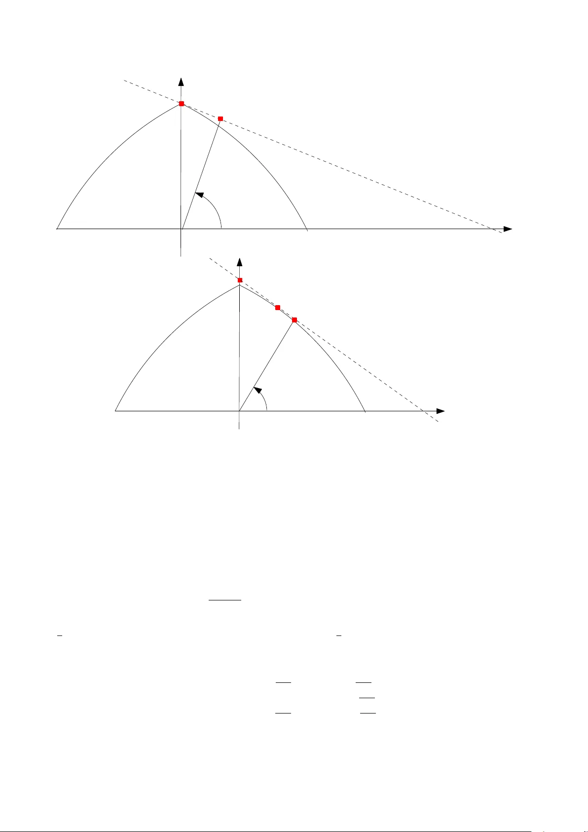
ELASTIC-NET REGULARIZA TION IN LEARNING THEOR Y C. DE MOL, E. DE VITO, L. R OSASCO Abstract. Within the framew ork of statistical learning theory we analyze in detail the so-called elastic-net regularization sc heme proposed by Zou and Hastie [45] for the selection of groups of correlated v ariables. T o in v estigate on the statistical properties of this sc heme and in particular on its consistency prop erties, we set up a suitable mathematical framework. Our setting is random-design regression where w e allo w the resp onse v ariable to b e vector-v alued and we consider prediction functions whic h are linear com bination of elemen ts ( fe atur es ) in an inﬁnite-dimensional dictionary . Under the assumption that the regression function admits a sparse representation on the dictionary , w e prov e that there exists a particular “ elastic-net r epr esentation ” of the regression function suc h that, if the n um b er of data increases, the elastic-net estimator is consisten t not only for prediction but also for v ariable/feature selection. Our results include ﬁnite- sample bounds and an adaptiv e sc heme to select the regularization parameter. Moreov er, using conv ex analysis to ols, we derive an iterative thresholding algorithm for computing the elastic-net solution whic h is diﬀerent from the optimization pro cedure originally prop osed in [45]. 1. Introduction W e consider the standard framew ork of sup ervised learning, that is nonparametric regression with random design. In this setting, there is an input-output pair ( X , Y ) ∈ X × Y with unknown probabilit y distribution P , and the goal is to ﬁnd a prediction function f n : X → Y , based on a training set ( X 1 , Y 1 ) , . . . , ( X n , Y n ) of n indep enden t random pairs distributed as ( X , Y ). A go od solution f n is such that, given a new input x ∈ X , the v alue f n ( x ) is a go o d prediction of the true output y ∈ Y . When choosing the square loss to measure the quality of the prediction, as we do throughout this pap er, this means that the exp ected risk E  | Y − f n ( X ) | 2  is smal l , or, in other words, that f n is a go o d approximation of the regression function f ∗ ( x ) = E [ Y | X = x ] minimizing this risk. In man y learning problems, a ma jor goal b esides prediction is that of sele cting the vari- ables that are r elevant to achieve go o d pr e dictions . In the problem of v ariable selection we are given a set ( ψ γ ) γ ∈ Γ of functions from the input space X into the output space Y and w e aim at selecting those functions whic h are needed to represen t the regression function, where the r epr esentation is typically given b y a linear com bination. The set ( ψ γ ) γ ∈ Γ is usually called dictionary and its elements fe atur es . W e can think of the features as mea- suremen ts used to represent the input data, as providing some relev ant parameterization of the input space, or as a (p ossibly ov ercomplete) dictionary of functions used to rep- resen t the prediction function. In mo dern applications, the num b er p of features in the dictionary is usually very large, p ossibly muc h larger that the num b er n of examples in the training set. This situation is often referred to as the “large p , small n paradigm” [9], and a key to obtain a meaningful solution in suc h case is the requirement that the prediction function f n is a linear com bination of only a few elements in the dictionary , i.e. that f n admits a sp arse represen tation. Date : Octob er 23, 2018. 1 2 C. DE MOL, E. DE VITO, L. ROSASCO The ab o v e setting can be illustrated by tw o examples of applications we are currently w orking on and which provide an underlying motiv ation for the theoretical framew ork dev elop ed in the present pap er. The ﬁrst application is a classiﬁcation problem in com- puter vision, namely face detection [17, 19, 18]. The training set con tains images of faces and non-faces and each image is represen ted b y a very large redundant set of features capturing the lo cal geometry of faces, for example wa velet-lik e dictionaries or other lo cal descriptors. The aim is to ﬁnd a go o d predictor able to detect faces in new images. The second application is the analysis of microarray data, where the features are the expression lev el measurements of the genes in a giv en sample or patient, and the output is either a classiﬁcation lab el discriminating b etw een tw o or more pathologies or a con tinuous index indicating, for example, the gra vity of an illness. In this problem, besides prediction of the output for examples-to-come, another imp ortan t goal is the identiﬁcation of the features that are the most relev ant to build the estimator and would constitute a gene signature for a certain disease [15, 4]. In both applications, the num b er of features we ha ve to deal with is muc h larger than the n umber of examples and assuming sparsity of the solution is a very natural requirement. The problem of v ariable/feature selection has a long history in statistics and it is kno wn that the brute-force approach (trying all possible subsets of features), though theoretically app ealing, is computationally unfeasible. A ﬁrst strategy to ov ercome this problem is pro vided b y greedy algorithms. A second route, whic h we follow in this pap er, mak es use of sparsit y-based regularization sc hemes (con vex relaxation metho ds). The most well- kno wn example of suc h schemes is probably the so-called L asso r e gr ession [38] – also referred to in the signal pro cessing literature as Basis Pursuit Denoising [13] – where a co eﬃcien t vector β n is estimated as the minimizer of the empirical risk p enalized with the ` 1 -norm, namely β n = argmin β =( β γ ) γ ∈ Γ 1 n n X i =1 | Y i − f β ( X i ) | 2 + λ X γ ∈ Γ | β γ | ! , where f β = P γ ∈ Γ β γ ψ γ , λ is a suitable p ositiv e regularization parameter and ( ψ γ ) γ ∈ Γ a giv en set of features. An extension of this approac h, called bridge r e gr ession , amoun ts to replacing the ` 1 -p enalt y b y an ` p -p enalt y [23]. It has been sho wn that this kind of p enalt y can still achiev e sparsit y when p is bigger, but very close to 1 (see [26]). F or this class of techniques, b oth consistency and computational asp ects ha ve b een studied. Non-asymptotic bounds within the framew ork of statistical learning hav e b een studied in sev eral pap ers [25, 8, 28, 37, 24, 39, 44, 26]. A common feature of these results is that they assume that the dictionary is ﬁnite (with cardinalit y p ossibly depending on the n umber of examples) and satisﬁes some assumptions ab out the linear indep endence of the relev an t features – see [26] for a discussion on this p oin t – whereas Y is usually assumed to b e R . Sev eral n umerical algorithms ha v e also been prop osed to solv e the optimization problem underlying Lasso regression and are based e.g. on quadratic programming [13], on the so-called LARS algorithm [20] or on iterativ e soft-thresholding (see [14] and references therein). Despite of its success in many applications, the Lasso strategy has some drawbac k in v ariable selection problems where there are highly correlated features and we need to iden tify all the relev an t ones. This situation is of uttermost imp ortance for e.g. microarra y data analysis since, as w ell-known, there is a lot of functional dependency b et w een genes whic h are organized in small in teracting net works. The identiﬁcation of suc h groups of correlated genes inv olv ed in a sp eciﬁc pathology is desirable to make progress in the understanding of the underlying biological mec hanisms. ELASTIC-NET REGULARIZA TION IN LEARNING THEOR Y 3 Motiv ated by microarra y data analysis, Zou and Hastie [45] prop osed the use of a p enalt y whic h is a w eighted sum of the ` 1 -norm and the square of the ` 2 -norm of the co eﬃcien t vector β . The ﬁrst term enforces the sparsity of the solution, whereas the second term ensures demo cracy among groups of correlated v ariables. In [45] the corresp onding metho d is called (naive) elastic net . The method allo ws to select groups of correlated features when the groups are not known in adv ance (algorithms to enforce group-sparsity with pr e assigne d groups of v ariables hav e b een prop osed in e.g. [31, 42, 22] using other t yp es of p enalties). In the presen t pap er w e study sev eral prop erties of the elastic-net regularization sc heme for v ector-v alued regression in a random design. In particular, w e prov e consistency under some adaptiv e and non-adaptiv e c hoices for the regularization parameter. As concerns v ariable selection, we assess the accuracy of our estimator for the vector β with resp ect to the ` 2 -norm, whereas the prediction abilit y of the corresp onding function f n = f β n is measured b y the exp ected risk E  | Y − f n ( X ) | 2  . T o derive such error b ounds, we c haracterize the solution of the v ariational problem underlying elastic-net regularization as the ﬁxed p oin t of a con tractiv e map and, as a b ypro duct, w e deriv e an explicit iterative thresholding pro cedure to compute the estimator. As explained b elo w, in the presence of highly collinear features, the presence of the ` 2 -p enalt y , b esides enforcing group ed selection, is crucial to ensure stabilit y with resp ect to random sampling. In the remainder of this section, w e deﬁne the main ingredients for elastic-net regular- ization within our general framew ork, discuss the underlying motiv ations for the metho d and then outline the main results established in the paper. As an extension of the setting originally prop osed in [45], w e allo w the dictionary to ha ve an inﬁnite num b er of features. In suc h case, to cop e with inﬁnite sums, we need some assumptions on the co eﬃcien ts. W e assume that the prediction function w e ha ve to determine is a linear combination of the features ( ψ γ ) γ ∈ Γ in the dictionary and that the series f β ( x ) = X γ ∈ Γ β γ ψ γ ( x ) , con verges absolutely for all x ∈ X and for all sequences β = ( β γ ) γ ∈ Γ satisfying P γ ∈ Γ u γ β 2 γ < ∞ , where u γ are given p ositiv e weigh ts. The latter constrain t can b e viewed as a con- strain t on the r e gularity of the functions f β w e use to appro ximate the regression function. F or inﬁnite-dimensional sets, as for example wa velet bases or splines, suitable c hoices of the weigh ts corresp ond to the assumption that f β is in a Sob olev space (see Section 2 for more details ab out this p oin t). Such requiremen t of regularit y is common when deal- ing with inﬁnite-dimensional spaces of functions, as it happ ens in approximation theory , signal analysis and inv erse problems. T o ensure the conv ergence of the series deﬁning f β , we assume that (1) X γ ∈ Γ | ψ γ ( x ) | 2 u γ is ﬁnite for all x ∈ X. Notice that for ﬁnite dictionaries, the series b ecomes a ﬁnite sum and the previous con- dition as w ell as the introduction of weigh ts b ecome superﬂuous. T o simplify the notation and the form ulation of our results, and without any loss in generalit y , we will in the following rescale the features b y deﬁning ϕ γ = ψ γ / √ u γ , so that on this r esc ale d dictionary , f β = P γ ∈ Γ ˜ β γ ϕ γ will b e represented by means of a vector ˜ β γ = √ u γ β γ b elonging to ` 2 ; the condition (1) then b ecomes P γ ∈ Γ | ϕ γ ( x ) | 2 < + ∞ , for all x ∈ X . F rom no w on, w e will only use this rescaled representation and we drop the tilde on the vector β . 4 C. DE MOL, E. DE VITO, L. ROSASCO Let us now deﬁne our estimator as the minimizer of the empirical risk p enalized with a (weigh ted) elastic-net p enalt y , that is, a combination of the squared ` 2 -norm and of a w eighted ` 1 -norm of the vector β . More precisely , we deﬁne the elastic-net p enalty as follo ws. Deﬁnition 1. Giv en a family ( w γ ) γ ∈ Γ of w eights w γ ≥ 0 and a parameter ε ≥ 0, let p ε : ` 2 → [0 , ∞ ] b e deﬁned as (2) p ε ( β ) = X γ ∈ Γ ( w γ | β γ | + εβ 2 γ ) whic h can also b e rewritten as p ε ( β ) = k β k 1 ,w + ε k β k 2 2 , where k β k 1 ,w = P γ ∈ Γ w γ | β γ | . The weigh ts w γ allo w us to enforce more or less sparsit y on diﬀeren t groups of features. W e assume that they are prescribed in a given problem, so that we do not need to explicitly indicate the dep endence of p ε ( β ) on these w eigh ts. The elastic-net estimator is deﬁned b y the following minimization problem. Deﬁnition 2. Giv en λ > 0, let E λ n : ` 2 → [0 , + ∞ ] b e the empirical risk p enalized by the p enalt y p ε ( β ) (3) E λ n ( β ) = 1 n n X i =1 | Y i − f β ( X i ) | 2 + λp ε ( β ) , and let β λ n ∈ ` 2 b e the or a minimizer of (3) on ` 2 (4) β λ n = argmin β ∈ ` 2 E λ n ( β ) . The positive parameter λ is a regularization parameter controlling the trade-oﬀ b etw een the empirical error and the penalty . Clearly , β λ n also dep ends on the parameter ε , but we do not write explicitly this dep endence since ε will alwa ys b e ﬁxed. Setting ε = 0 in (3), w e obtain as a sp ecial case an inﬁnite-dimensional extension of the Lasso regression sc heme. On the other hand, setting w γ = 0 , ∀ γ , the metho d reduces to ` 2 -regularized least-squares regression – also referred to as ridge r e gr ession – with a generalized linear mo del. The ` 1 -p enalt y has selection capabilities since it enforces sparsity of the solution, whereas the ` 2 -p enalt y induces a linear shrink age on the co eﬃcien ts leading to stable solutions. The p ositiv e parameter ε con trols the trade-oﬀ betw een the ` 1 -p enalt y and the ` 2 -p enalt y . W e will show that, if ε > 0, the minimizer β λ n alw ays exists and is unique. In the pap er w e will fo cus on the case ε > 0. Some of our results, ho wev er, still hold for ε = 0, possibly under some supplemen tary conditions, as will b e indicated in due time. As previously men tioned one of the main adv an tage of the elastic-net p enalt y is that it allows to achiev e stability with resp ect to random sampling. T o illustrate this prop- ert y more clearly , w e consider a to y example where the (rescaled) dictionary has only t wo elemen ts ϕ 1 and ϕ 2 with w eigh ts w 1 = w 2 = 1. The eﬀect of random sampling is particularly dramatic in the presence of highly correlated features. T o illustrate this situ- ation, w e assume that ϕ 1 and ϕ 2 exhibit a sp ecial kind of linear dep endency , namely that they are linearly dep endent on the input data X 1 , . . . , X n : ϕ 2 ( X i ) = tan θ n ϕ 1 ( X i ) for all i = 1 , . . . , n , where we hav e parametrized the co eﬃcien t of prop ortionalit y by means of the angle θ n ∈ [0 , π / 2]. Notice that this angle is a random v ariable since it dep ends on the input data. Observ e that the minimizers of (3) must lie at a tangency point b et w een a lev el set of the empirical error and a lev el set of the elastic-net penalty . The lev el sets of the empirical error are all parallel straigh t lines with slope − cot θ n , as depicted by a dashed line in the ELASTIC-NET REGULARIZA TION IN LEARNING THEOR Y 5 Figure 1. The ε -ball with ε > 0 (solid line), the square ( ` 1 -ball), whic h is the ε -ball with ε = 0 (dashed line), and the disc ( ` 2 -ball), whic h is the ε -ball with ε → ∞ (dotted line). t wo panels of Figure 2, whereas the level sets of the elastic-net p enalt y are elastic-net b al ls ( ε -b al ls ) with cen ter at the origin and corners at the intersections with the axes, as depicted in Figure 1. When ε = 0, i.e. with a pure ` 1 -p enalt y (Lasso), the ε -ball is simply a squar e (dashed line in Figure 1) and we see that the unique tangency point will b e the top c orner if θ n > π / 4 (the p oin t T in the t wo panels of Figure 2), or the right c orner if θ n < π / 4. F or θ n = π / 4 (that is, when ϕ 1 and ϕ 2 coincide on the data), the minimizer of (3) is no longer unique since the level sets will touc h along an edge of the square. Now, if θ n randomly tilts around π / 4 (b ecause of the random sampling of the input data), w e see that the Lasso estimator is not stable since it randomly jumps b et ween the top and the righ t corner. If ε → ∞ , i.e. with a pure ` 2 -p enalt y (ridge regression), the ε -ball b ecomes a disc (dotted line in Figure 1) and the minimizer is the p oin t of the straight line ha ving minimal distance from the origin (the p oint Q in the tw o panels of Figure 2). The solution alwa ys exists, is stable under random p erturbations, but it is nev er sparse (if 0 < θ n < π / 2). The situation changes if w e consider the elastic-net estimator with ε > 0 (the corre- sp onding minimizer is the p oin t P in the tw o panels of Figure 2). The presence of the ` 2 -term ensures a smo oth and stable b ehavior when the Lasso estimator b ecomes unsta- ble. More precisely , let − cot θ + b e the slop e of the righ t tangent at the top corner of the elastic-net ball ( θ + > π / 4), and − cot θ − the slope of the upper tangen t at the righ t corner ( θ − < π / 4). As depicted in top panel of Figure 2, the minimizer will b e the top corner if θ n > θ + . It will b e the righ t corner if θ n < θ − . In b oth cases the elastic-net solution is sparse. On the other hand, if θ − ≤ θ n ≤ θ + the minimizer has b oth comp onen ts β 1 and β 2 diﬀeren t from zero – see the b ottom panel of Figure 2; in particular, β 1 = β 2 if θ n = π / 4. No w we observe that if θ n randomly tilts around π / 4, the solution smo othly mo ves b et ween the top corner and the right corner. How ev er, the price w e paid to get suc h stability is a decrease in sparsity , since the solution is sparse only when θ n 6∈ [ θ − , θ + ]. 6 C. DE MOL, E. DE VITO, L. ROSASCO P = T Q θ P Q θ T Figure 2. Estimators in the t wo-dimensional example: T =Lasso, P =elastic net and Q =ridge regression. T op panel: θ + < θ < π / 2. Bottom panel: π / 4 < θ < θ + . The previous elemen tary example could b e reﬁned in v arious w ays to sho w the essential role pla yed by the ` 2 -p enalt y to o v ercome the instability eﬀects inheren t to the use of the ` 1 -p enalt y for v ariable selection in a random-design setting. W e now conclude this introductory section b y a summary of the main results whic h will b e deriv ed in the core of the pap er. A key result will b e to show that for ε > 0, β λ n is the ﬁxed p oin t of the follo wing con tractive map β = 1 τ + ελ S λ (( τ I − Φ ∗ n Φ n ) β + Φ ∗ n Y ) where τ is a suitable relaxation constant, Φ ∗ n Φ n is the matrix with en tries (Φ ∗ n Φ n ) γ ,γ 0 = 1 n P n i =1 h ϕ γ ( X i ) , ϕ γ 0 ( X i ) i , Φ ∗ n Y is the vector (Φ ∗ n Y ) γ = 1 n P n i =1 h ϕ γ ( X i ) , Y i i ( h· , ·i denotes the scalar pro duct in the output space Y ). Moreo v er, S λ ( β ) is the soft-thresholding op erator acting comp onen t wise as follows [ S λ ( β )] γ =    β γ − λw γ 2 if β γ > λw γ 2 0 if | β γ | ≤ λw γ 2 β γ + λw γ 2 if β γ < − λw γ 2 . As a consequence of the Banach ﬁxed p oin t theorem, β λ n can b e computed by means of an iterativ e algorithm. This pro cedure is completely diﬀerent from the mo diﬁcation of the LARS algorithm used in [45] and is akin instead to the algorithm dev elop ed in [14]. ELASTIC-NET REGULARIZA TION IN LEARNING THEOR Y 7 Another interesting prop ert y whic h we will deriv e from the ab o ve equation is that the non-zero comp onen ts of β λ n are suc h that w γ ≤ C λ , where C is a constant dep ending on the data. Hence the only activ e features are those for whic h the corresponding w eigh t lies b elo w the threshold C /λ . If the features are organized into ﬁnite subsets of increasing complexit y (as it happ ens for example for w av elets) and the weigh ts tend to inﬁnit y with increasing feature complexit y , then the n umber of active features is ﬁnite and can b e determined for any given data set. Let us recall that in the case of ridge regression, the so-called r epr esenter the or em , see [41], ensures that w e only ha v e to solv e in practice a ﬁnite-dimensional optimization problem, ev en when the dictionary is inﬁnite-dimensional (as in k ernel metho ds). This is no longer true, ho w ever, with an ` 1 -t yp e regularization and, for practical purp oses, one w ould need to truncate inﬁnite dictionaries. A standard w ay to do this is to consider only a ﬁnite subset of m features, with m p ossibly dep ending on n – see for example [8, 24]. Notice that such procedure implicitly assumes some order in the features and makes sense only if the retained features are the most relev an t ones. F or example, in [5], it is assumed that there is a natural exhaustion of the hypothesis space with nested subspaces spanned by ﬁnite-dimensional subsets of features of increasing size. In our approac h w e adopt a diﬀeren t strategy , namely the enco ding of suc h information in the elastic-net p enalt y b y means of suitable w eigh ts in the ` 1 -norm. The main result of our pap er concerns the consistency for v ariable selection of β λ n . W e pro ve that, if the regularization parameter λ = λ n satisﬁes the conditions lim n →∞ λ n = 0 and lim n →∞ ( λ n √ n − 2 log n ) = + ∞ , then lim n →∞   β λ n n − β ε   2 = 0 with probability one , where the v ector β ε , whic h we call the elastic-net r epr esentation of f β , is the minimizer of min β ∈ ` 2 X γ ∈ Γ w γ | β γ | + ε X γ ∈ Γ | β γ | 2 ! sub ject to f β = f ∗ . The vector β ε exists and is unique pro vided that ε > 0 and the regression function f ∗ admits a sp arse r epr esentation on the dictionary , i.e. f ∗ = P γ ∈ Γ β ∗ γ ϕ γ for at least a vector β ∗ ∈ ` 2 suc h that P γ ∈ Γ w γ | β ∗ γ | is ﬁnite. Notice that, when the features are linearly dep enden t, there is a problem of identiﬁabilit y since there are man y v ectors β suc h that f ∗ = f β . The elastic-net regularization sc heme forces β λ n n to con verge to β ε . This is precisely what happ ens for linear inv erse problems where the regularized solution con verges to the minimum-norm solution of the least-squares problem. As a consequence of the ab o v e con vergence result, one easily deduces the consistency of the corresp onding prediction function f n := f β λ n n , that is, lim n →∞ E  | f n − f ∗ | 2  = 0 with probabilit y one. When the regression function do es not admit a sparse representation, we can still prov e the previous consistency result for f n pro vided that the linear span of the features is suﬃcien tly ric h. Finally , we use a data-driv en choice for the regularization parameter, based on the so-called balancing principle [6], to obtain non-asymptotic b ounds whic h are adaptiv e to the unkno wn regularit y of the regression function. The rest of the pap er is organized as follo ws. In Section 2, we set up the mathematical framew ork of the problem. In Section 3, we analyze the optimization problem underlying elastic-net regularization and the iterativ e thresholding pro cedure we prop ose to compute the estimator. Finally , Section 4 con tains the statistical analysis with our main results concerning the estimation of the errors on our estimators as well as their consistency prop- erties under appropriate a priori and adaptive strategies for c ho osing the regularization parameter. 8 C. DE MOL, E. DE VITO, L. ROSASCO 2. Ma thema tical setting of the problem 2.1. Notations and assumptions. In this section w e describ e the general setting of the regression problem w e w ant to solve and sp ecify all the required assumptions. W e assume that X is a separable metric space and that Y is a (real) separable Hilb ert space, with norm and scalar pro duct denoted respectively by | · | and h· , ·i . Typically , X is a subset of R d and Y is R . Recently , ho wev er, there has b een an increasing interest for v ector-v alued regression problems [29, 3] and m ultiple sup ervised learning tasks [30, 2 ]: in b oth settings Y is tak en to b e R m . Also inﬁnite-dimensional output spaces are of interest as e.g. in the problem of estimating of glycemic response during a time in terv al dep ending on the amoun t and type of fo o d; in suc h case, Y is the space L 2 or some Sob olev space. Other examples of applications in an inﬁnite-dimensional setting are giv en in [11]. Our ﬁrst assumption concerns the set of features. Assumption 1. The family of features ( ϕ γ ) γ ∈ Γ is a coun table set of measurable functions ϕ γ : X → Y such that ∀ x ∈ X k ( x ) = X γ ∈ Γ | ϕ γ ( x ) | 2 ≤ κ, (5) for some ﬁnite num b er κ . The index set Γ is coun table, but we do not assume any order. As for the conv ergence of series, we use the notion of summability: giv en a family ( v γ ) γ ∈ Γ of v ectors in a normed v ector space V , v = P γ ∈ Γ v γ means that ( v γ ) γ ∈ Γ is summable 1 with sum v ∈ V . Assumption 1 can b e seen as a condition on the class of functions that can b e recov ered b y the elastic-net sc heme. As already noted in the In tro duction, w e hav e at our disp osal an arbitrary (countable) dictionary ( ψ γ ) γ ∈ Γ of measurable functions, and we try to ap- pro ximate f ∗ with linear com binations f β ( x ) = P γ ∈ Γ β γ ψ γ ( x ) where the set of coeﬃcients ( β γ ) γ ∈ Γ satisﬁes some de c ay c ondition equiv alent to a r e gularity c ondition on the functions f β . W e make this condition precise b y assuming that there exists a sequence of p ositive w eights ( u γ ) γ ∈ Γ suc h that P γ ∈ Γ u γ β 2 γ < ∞ and, for an y of such vectors β = ( β γ ) γ ∈ Γ , that the series deﬁning f β con verges absolutely for all x ∈ X . These t wo facts follow from the requirement that the set of rescaled features ϕ γ = ψ γ √ u γ satisﬁes P γ ∈ Γ | ϕ γ ( x ) | 2 < ∞ . Condition (5) is a little bit stronger since it requires that sup x ∈X P γ ∈ Γ | ϕ γ ( x ) | 2 < ∞ , so that we also hav e that the functions f β are b ounded. T o simplify the notation, in the rest of the pap er, w e only use the (rescaled) features ϕ γ and, with this c hoice, the regularit y condition on the co eﬃcien ts ( β γ ) γ ∈ Γ b ecomes P γ ∈ Γ β 2 γ < ∞ . An example of features satisfying the condition (5) is given b y a family of r esc ale d w av elets on X = [0 , 1]. Let { ψ j k | j = 0 , 1 . . . ; k ∈ ∆ j } b e a orthonormal w av elet basis in L 2 ([0 , 1]) with regularit y C r , r > 1 2 , where for j ≥ 1 { ψ j k | k ∈ ∆ j } is the orthonormal w av elet basis (with suitable b oundary conditions) spanning the detail space at lev el j . T o simplify notation, it is assumed that the set { ψ 0 k | k ∈ ∆ 0 } con tains b oth the wa velets and the scaling functions at level j = 0. Fix s suc h that 1 2 < s < r and let ϕ j k = 2 − j s ψ j k . 1 That is, for all η > 0, there is a ﬁnite subset Γ 0 ⊂ Γ such that    v − P γ ∈ Γ 0 v γ    V ≤ η for all ﬁnite subsets Γ 0 ⊃ Γ 0 . If Γ = N , the notion of summabilit y is equiv alent to requiring the series to conv erge unconditionally (i.e. its terms can b e permuted without aﬀecting conv ergence). If the v ector space is ﬁnite-dimensional, summabilit y is equiv alent to absolute conv ergence, but in the inﬁnite-dimensional setting, there are summable series whic h are not absolutely con v ergen t. ELASTIC-NET REGULARIZA TION IN LEARNING THEOR Y 9 Then ∞ X j =0 X k ∈ ∆ j | ϕ j k ( x ) | 2 = ∞ X j =0 X k ∈ ∆ j 2 − 2 j s | ψ j k ( x ) | 2 ≤ C ∞ X j =0 2 − 2 j s 2 j = C 1 1 − 2 1 − 2 s = κ, where C is a suitable constan t dep ending on the num b er of wa v elets that are non-zero at a p oin t x ∈ [0 , 1] for a giv en lev el j , and on the maxim um v alues of the scaling function and of the mother wa velet; see [1] for a similar setting. Condition (5) allo ws to deﬁne the hypothesis space in whic h w e searc h for the estimator. Let ` 2 b e the Hilbert space of the families ( β γ ) γ ∈ Γ of real num b ers suc h that P γ ∈ Γ β 2 γ < ∞ , with the usual scalar pro duct h· , ·i 2 and the corresponding norm k·k 2 . W e will denote by ( e γ ) γ ∈ Γ the canonical basis of ` 2 and b y supp( β ) = { γ ∈ Γ | β γ 6 = 0 } the supp ort of β . The Cauc hy-Sc hw arz inequality and the condition (5) ensure that, for an y β = ( β γ ) γ ∈ Γ ∈ ` 2 , the series X γ ∈ Γ β γ ϕ γ ( x ) = f β ( x ) is summable in Y uniformly on X with (6) sup x ∈X | f β ( x ) | ≤ k β k 2 κ 1 2 . Later on, in Prop osition 3, we will show that the hypothesis space H = { f β | β ∈ ` 2 } is then a vector-v alued repro ducing k ernel Hilb ert space on X with a b ounded kernel [12], and that ( ϕ γ ) γ ∈ Γ is a normalized tigh t frame for H . In the example of the w av elet features one can easily chec k that H is the Sob olev space H s on [0 , 1] and k β k 2 is equiv alent to k f β k H s . The second assumption concerns the regression mo del. Assumption 2. The random couple ( X, Y ) in X × Y obeys the regression model Y = f ∗ ( X ) + W where (7) f ∗ = f β ∗ for some β ∗ ∈ ` 2 with X γ ∈ Γ w γ | β ∗ γ | < + ∞ and E [ W | X ] = 0 (8) E  exp  | W | L  − | W | L − 1    X  ≤ σ 2 2 L 2 (9) with σ , L > 0. The family ( w γ ) γ ∈ Γ are the positive w eights deﬁning the elastic-net penalty p ε ( β ) in (2). Observ e that f ∗ = f β ∗ is alwa ys a bounded function b y (6). Moreo ver the condition (7) is a further regularit y condition on the regression function and will not b e needed for some of the results derived in the paper. Assumption (9) is satisﬁed b y bounded, Gaussian or sub-Gaussian noise. In particular, it implies E [ | W | m | X ] ≤ 1 2 m ! σ 2 L m − 2 , ∀ m ≥ 2 , (10) see [40], so that W has a ﬁnite second momen t. It follo ws that Y has a ﬁnite ﬁrst moment and (8) implies that f ∗ is the regression function E [ Y | X = x ]. 10 C. DE MOL, E. DE VITO, L. ROSASCO Condition (7) controls both the sparsit y and the regularity of the regression function. If inf γ ∈ Γ w γ = w 0 > 0, it is suﬃcien t to require that k β ∗ k 1 ,w is ﬁnite. Indeed, the H¨ older inequalit y giv es that (11) k β k 2 ≤ 1 w 0 k β k 1 ,w . If w 0 = 0, w e also need k β ∗ k 2 to b e ﬁnite. In the example of the (rescaled) wa v elet features a natural choice for the w eigh ts is w j k = 2 j a for some a ∈ R , so that k β k 1 ,w is equiv alent to the norm k f β k B ˜ s 1 , 1 , with ˜ s = a + s + 1 2 , in the Besov space B ˜ s 1 , 1 on [0 , 1] (for more details, see e.g. the app endix in [14]). In suc h a case, (7) is equiv alen t to requiring that f ∗ ∈ H s ∩ B ˜ s 1 , 1 . Finally , our third assumption concerns the training sample. Assumption 3. The sequence of random pairs ( X n , Y n ) n ≥ 1 are indep enden t and iden ti- cally distributed ( i.i.d. ) according to the distribution of ( X , Y ). In the follo wing, w e let P b e the probability distribution of ( X , Y ), and L 2 Y ( P ) b e the Hilb ert space of (measurable) functions f : X × Y → Y with the norm k f k 2 P = Z X ×Y | f ( x, y ) | 2 dP ( x, y ) . With a sligh t abuse of notation, w e regard the random pair ( X, Y ) as a function on X × Y , that is, X ( x, y ) = x and Y ( x, y ) = y . Moreo ver, we denote by P n = 1 n P n i =1 δ X i ,Y i the empirical distribution and b y L 2 Y ( P n ) the corresp onding (ﬁnite-dimensional) Hilb ert space with norm k f k 2 n = 1 n n X i =1 | f ( X i , Y i ) | 2 . 2.2. Op erators deﬁned by the set of features. The choice of a quadratic loss function and the Hilb ert structure of the h yp othesis space suggest to use some to ols from the theory of linear op erators. In particular, the function f β dep ends linearly on β and can b e regarded as an elemen t of both L 2 Y ( P ) and of L 2 Y ( P n ). Hence it deﬁnes tw o op erators, whose prop erties are summarized by the next tw o prop ositions, based on the following lemma. Lemma 1. F or any ﬁxe d x ∈ X , the map Φ x : ` 2 → Y deﬁne d by Φ x β = X γ ∈ Γ ϕ γ ( x ) β γ = f β ( x ) is a Hilb ert-Schmidt op er ator, its adjoint Φ ∗ x : Y → ` 2 acts as (12) (Φ ∗ x y ) γ = h y , ϕ γ ( x ) i γ ∈ Γ y ∈ Y . In p articular Φ ∗ x Φ x is a tr ac e-class op er ator with (13) T r (Φ ∗ x Φ x ) ≤ κ. Mor e over, Φ ∗ X Y is a ` 2 -value d r andom variable with (14) k Φ ∗ X Y k 2 ≤ κ 1 2 | Y | , and Φ ∗ X Φ X is a L HS -value d r andom variable with (15) k Φ ∗ X Φ X k HS ≤ κ, wher e L HS denotes the sep ar able Hilb ert sp ac e of the Hilb ert-Schmidt op er ators on ` 2 , and k·k HS is the Hilb ert-Schmidt norm. ELASTIC-NET REGULARIZA TION IN LEARNING THEOR Y 11 Pr o of. Clearly Φ x is a linear map from ` 2 to Y . Since Φ x e γ = ϕ γ ( x ), we ha ve X γ ∈ Γ | Φ x e γ | 2 = X γ ∈ Γ | ϕ γ ( x ) | 2 ≤ κ, so that Φ x is a Hilb ert-Sc hmidt operator and T r (Φ ∗ x Φ x ) ≤ κ by (5). Moreo ver, giv en y ∈ Y and γ ∈ Γ (Φ ∗ x y ) γ = h Φ ∗ x y , e γ i 2 = h y , ϕ γ ( x ) i whic h is (12). Finally , since X and Y are separable, the map ( x, y ) → h y , ϕ γ ( x ) i is measurable, then (Φ ∗ X Y ) γ is a real random v ariable and, since ` 2 is separable, Φ ∗ X Y is ` 2 -v alued random v ariable with k Φ ∗ X Y k 2 2 = X γ ∈ Γ h Y , ϕ γ ( X ) i 2 ≤ κ | Y | 2 . A similar proof holds for Φ ∗ X Φ X , recalling that an y trace-class operator is in L HS and k Φ ∗ X Φ X k HS ≤ T r (Φ ∗ X Φ X ).  The following prop osition deﬁnes the distribution-dep endent op erator Φ P as a map from ` 2 in to L 2 Y ( P ). Prop osition 1. The map Φ P : ` 2 → L 2 Y ( P ) , deﬁne d by Φ P β = f β , is a Hilb ert-Schmidt op er ator and Φ ∗ P Y = E [Φ ∗ X Y ] (16) Φ ∗ P Φ P = E [Φ ∗ X Φ X ] (17) T r (Φ ∗ P Φ P ) = E [ k ( X )] ≤ κ. (18) Pr o of. Since f β is a b ounded (measurable) function, f β ∈ L 2 Y ( P ) and X γ ∈ Γ k Φ P e γ k 2 P = X γ ∈ Γ E  | ϕ γ ( X ) | 2  = E [ k ( X )] ≤ κ. Hence Φ P is a Hilb ert-Sc hmidt op erator with T r (Φ ∗ P Φ P ) = P γ ∈ Γ k Φ P e γ k 2 P so that (18) holds. By (9) W has a ﬁnite second moment and by (6) f ∗ = f β ∗ is a b ounded function, hence Y = f ∗ ( X ) + W is in L 2 Y ( P ). No w for an y β ∈ ` 2 w e ha ve h Φ ∗ P Y , β i 2 = h Y , Φ P β i P = E [ h Y , Φ X β i ] = E [ h Φ ∗ X Y , β i 2 ] . On the other hand, by (14), Φ ∗ X Y has ﬁnite exp ectation, so that (16) follo ws. Finally , giv en β , β 0 ∈ ` 2 h Φ ∗ P Φ P β 0 , β i 2 = h Φ P β 0 , Φ P β i P = E [ h Φ X β 0 , Φ X β i ] = E [ h Φ ∗ X Φ X β 0 , β i 2 ] so that (17) is clear, since Φ ∗ X Φ X has ﬁnite exp ectation as a consequence of the fact that it is a b ounded L HS -v alued random v ariable.  Replacing P by the empirical measure w e get the sample version of the op erator. 12 C. DE MOL, E. DE VITO, L. ROSASCO Prop osition 2. The map Φ n : ` 2 → L 2 Y ( P n ) deﬁne d by Φ n β = f β is Hilb ert-Schmidt op er ator and Φ ∗ n Y = 1 n n X i =1 Φ ∗ X i Y i (19) Φ ∗ n Φ n = 1 n n X i =1 Φ ∗ X i Φ X i (20) T r (Φ ∗ n Φ n ) = 1 n n X i =1 k ( X i ) ≤ κ. (21) The pro of of Proposition 2 is analogous to the proof of Prop osition 1, except that P is to b e replaced b y P n . By (12) with y = ϕ γ 0 ( x ), w e hav e that the matrix elements of the op erator Φ ∗ x Φ x are (Φ ∗ x Φ x ) γ γ 0 = h ϕ γ 0 ( x ) , ϕ γ ( x ) i so that Φ ∗ n Φ n is the empirical mean of the Gram matrix of the set ( ϕ γ ) γ ∈ Γ , whereas Φ ∗ P Φ P is the corresp onding mean with resp ect to the distribution P . Notice that if the features are linearly dep endent in L 2 Y ( P n ), the matrix Φ ∗ n Φ n has a non- trivial k ernel and hence is not in vertible. More imp ortan t, if Γ is countably inﬁnite, Φ ∗ n Φ n is a compact op erator, so that its inv erse (if it exists) is not b ounded. On the contrary , if Γ is ﬁnite and ( ϕ γ ) γ ∈ Γ are linearly indep enden t in L 2 Y ( P n ), then Φ ∗ n Φ n is in vertible. A similar reasoning holds for the matrix Φ ∗ P Φ P . T o con trol whether these matrices hav e a b ounded in v erse or not, w e in tro duce a lo wer sp ectral b ound κ 0 ≥ 0, such that κ 0 ≤ inf β ∈ ` 2 | k β k 2 =1 h Φ ∗ P Φ P β , β i 2 and, with probabilit y 1, κ 0 ≤ inf β ∈ ` 2 | k β k 2 =1 h Φ ∗ n Φ n β , β i 2 . Clearly we can ha v e κ 0 > 0 only if Γ is ﬁnite and the features ( ϕ γ ) γ ∈ Γ are linearly indep enden t both in L 2 Y ( P n ) and L 2 Y ( P ). On the other hand, (18) and (21) giv e the crude upper sp ectral b ounds sup β ∈ ` 2 | k β k 2 =1 h Φ ∗ P Φ P β , β i 2 ≤ κ, sup β ∈ ` 2 | k β k 2 =1 h Φ ∗ n Φ n β , β i 2 ≤ κ. One could impro v e these estimates by means of a tigh t b ound on the largest eigenv alue of Φ ∗ P Φ P . W e end this section b y showing that, under the assumptions we made, a structure of repro ducing kernel Hilb ert space emerges naturally . Let us denote by Y X the space of functions from X to Y . Prop osition 3. The line ar op er ator Φ : ` 2 → Y X , Φ β = f β , is a p artial isometry fr om ` 2 onto the ve ctor-value d r epr o ducing kernel Hilb ert sp ac e H on X , with r epr o ducing kernel K : X × X → L ( Y ) (22) K ( x, t ) y = (Φ x Φ ∗ t ) y = X γ ∈ Γ ϕ γ ( x ) h y , ϕ γ ( t ) i x, t ∈ X , y ∈ Y , the nul l sp ac e of Φ is (23) k er Φ = { β ∈ ` 2 | X γ ∈ Γ ϕ γ ( x ) β γ = 0 ∀ x ∈ X } , ELASTIC-NET REGULARIZA TION IN LEARNING THEOR Y 13 and the family ( ϕ γ ) γ ∈ Γ is a normalize d tight fr ame in H , namely X γ ∈ Γ | h f , ϕ γ i H | 2 = k f k 2 H ∀ f ∈ H . Conversely, let H b e a ve ctor-value d r epr o ducing kernel Hilb ert sp ac e with r epr o ducing kernel K such that K ( x, x ) : Y → Y is a tr ac e-class op er ator for al l x ∈ X , with tr ac e b ounde d by κ . If ( ϕ γ ) γ ∈ Γ is a normalize d tight fr ame in H , then (5) holds. Pr o of. Prop osition 2.4 of [12] (with K = Y , b H = ` 2 , γ ( x ) = Φ ∗ x and A = Φ) gives that Φ is a partial isometry from ` 2 on to the repro ducing k ernel Hilbert space H , with repro ducing k ernel K ( x, t ). Eq. (23) is clear. Since Φ is a partial isometry with range H and Φ e γ = ϕ γ where ( e γ ) γ ∈ Γ is a basis in ` 2 , then ( ϕ γ ) γ ∈ Γ is normalized tigh t frame in H . T o sho w the conv erse result, giv en x ∈ X and y ∈ Y , w e apply the deﬁnition of a normalized tigh t frame to the function K x y deﬁned by ( K x y )( t ) = K ( t, x ) y . K x y belongs to H by deﬁnition of a repro ducing kernel Hilb ert space and is suc h that the follo wing repro ducing prop ert y holds h f , K x y i H = h f ( x ) , y i for an y f ∈ H . Then h K ( x, x ) y , y i = k K x y k 2 H = X γ ∈ Γ | h K x y , ϕ γ i H | 2 = X γ ∈ Γ | h y , ϕ γ ( x ) i | 2 , where we used twice the repro ducing prop ert y . Now, if ( y i ) i ∈ I is a basis in Y and x ∈ X X γ ∈ Γ | ϕ γ ( x ) | 2 = X γ ∈ Γ X i ∈ I | h y i , ϕ γ ( x ) i | 2 = X i ∈ I h K ( x, x ) y i , y i i = T r ( K ( x, x )) ≤ κ.  3. Minimiza tion of the elastic-net functional In this section, we study the prop erties of the elastic net estimator β λ n deﬁned b y (4). First of all, we characterize the minimizer of the elastic-net functional (3) as the unique ﬁxed p oin t of a contractiv e map. Moreo ver, we characterize some sparsit y prop erties of the estimator and prop ose a natural iterativ e soft-thresholding algorithm to compute it. Our algorithmic approac h is totally diﬀeren t from the method prop osed in [45], where β λ n is computed by ﬁrst reducing the problem to the case of a pure ` 1 p enalt y and then applying the LARS algorithm [20]. In the follo wing w e mak e use the of the follo wing v ector notation. Giv en a sample of n i.i.d. observ ations ( X 1 , Y 1 ) , . . . , ( X n , Y n ), and using the op erators deﬁned in the previous section, we can rewrite the elastic-net functional (3) as (24) E λ n ( β ) = k Φ n β − Y k 2 n + λp ε ( β ) , where the p ε ( · ) is the elastic net p enalt y deﬁned b y (2). 3.1. Fixed p oint equation. The main diﬃcult y in minimizing (24) is that the functional is not diﬀeren tiable b ecause of the presence of the ` 1 -term in the p enalty . Nonetheless the conv exit y of suc h term enables us to use to ols from sub diﬀeren tial calculus. Recall that, if F : ` 2 → R is a conv ex functional, the subgradient at a point β ∈ ` 2 is the set of elemen ts η ∈ ` 2 suc h that F ( β + β 0 ) ≥ F ( β ) + h η , β 0 i 2 ∀ β 0 ∈ ` 2 . 14 C. DE MOL, E. DE VITO, L. ROSASCO The subgradien t at β is denoted b y ∂ F ( β ), see [21]. W e compute the subgradient of the con vex functional p ε ( β ), using the follo wing deﬁnition of sgn( t ) (25)    sgn( t ) = 1 if t > 0 sgn( t ) ∈ [ − 1 , 1] if t = 0 sgn( t ) = − 1 if t < 0 . W e ﬁrst state the follo wing lemma. Lemma 2. The functional p ε ( · ) is a c onvex, lower semi-c ontinuous (l.s.c.) functional fr om ` 2 into [0 , ∞ ] . Given β ∈ ` 2 , a ve ctor η ∈ ∂ p ε ( β ) if and only if η γ = w γ sgn( β γ ) + 2 εβ γ ∀ γ ∈ Γ and X γ ∈ Γ η 2 γ < + ∞ . Pr o of. Deﬁne the map F : Γ × R → [0 , ∞ ] F ( γ , t ) = w γ | t | + εt 2 . Giv en γ ∈ Γ, F ( γ , · ) is a conv ex, contin uous function and its subgradien t is ∂ F ( γ , t ) = { τ ∈ R | τ = w γ sgn( t ) + 2 εt } , where we used the fact that the subgradien t of | t | is given b y sgn( t ). Since p ε ( β ) = X γ ∈ Γ F ( γ , β γ ) = sup Γ 0 ﬁnite X γ ∈ Γ 0 F ( γ , β γ ) and β 7→ β γ is contin uous, a standard result of conv ex analysis [21] ensures that p ε ( · ) is con vex and low er semi-con tinuous. The computation of the subgradient is standard. Given β ∈ ` 2 and η ∈ ∂ p ε ( β ) ⊂ ` 2 , by the deﬁnition of a subgradient, X γ ∈ Γ F ( γ , β γ + β 0 γ ) ≥ X γ ∈ Γ F ( γ , β γ ) + X γ ∈ Γ η γ β 0 γ ∀ β 0 ∈ ` 2 . Giv en γ ∈ Γ, c ho ose β 0 = te γ with t ∈ R , it follows that η γ b elongs to the subgradient of F ( γ , β γ ), that is, (26) η γ = w γ sgn( β γ ) + 2 εβ γ . Con versely , if (26) holds for all γ ∈ Γ, by deﬁnition of a subgradient F ( γ , β γ + β 0 γ ) ≥ F ( γ , β γ ) + η γ β 0 γ . By summing o ver γ ∈ Γ and taking in to accoun t the fact that ( η γ β γ ) γ ∈ Γ ∈ ` 1 , then p ε ( β + β 0 ) ≥ p ε ( β ) + h η , β 0 i 2 .  T o state our main result ab out the c haracterization of the minimizer of (24), w e need to introduce the soft-thresholding function S λ : R → R , λ > 0 whic h is deﬁned b y (27) S λ ( t ) =    t − λ 2 if t > λ 2 0 if | t | ≤ λ 2 t + λ 2 if t < − λ 2 , and the corresp onding nonlinear thresholding operator S λ : ` 2 → ` 2 acting component wise as (28) [ S λ ( β )] γ = S λw γ ( β γ ) . ELASTIC-NET REGULARIZA TION IN LEARNING THEOR Y 15 W e note that the soft-thresholding op erator satisﬁes S aλ ( aβ ) = a S λ ( β ) a > 0 , β ∈ ` 2 , (29) k S λ ( β ) − S λ ( β 0 ) k 2 ≤ k β − β 0 k 2 β , β 0 ∈ ` 2 . (30) These prop erties are immediate consequences of the fact that S aλ ( at ) = a S λ ( t ) a > 0 , t ∈ R |S λ ( t ) − S λ ( t 0 ) | ≤ | t − t 0 | t, t 0 ∈ R . Notice that (30) with β 0 = 0 ensures that S λ ( β ) ∈ ` 2 for all β ∈ ` 2 . W e are ready to pro ve the following theorem. Theorem 1. Given ε ≥ 0 and λ > 0 , a ve ctor β ∈ ` 2 is a minimizer of the elastic-net functional (3) if and only if it solves the nonline ar e quation (31) 1 n n X i =1 h Y i − (Φ n β )( X i ) , ϕ γ ( X i ) i − ελβ γ = λ 2 w γ sgn( β γ ) ∀ γ ∈ Γ , or, e quivalently, (32) β = S λ ((1 − ελ ) β + Φ ∗ n ( Y − Φ n β )) . If ε > 0 the solution always exists and is unique. If ε = 0 , κ 0 > 0 and w 0 = inf γ ∈ Γ w γ > 0 , the solution stil l exists and is unique. Pr o of. If ε > 0 the functional E λ n is strictly con vex, ﬁnite at 0, and it is co erciv e by E λ n ( β ) ≥ p ε ( β ) ≥ λε k β k 2 2 . Observing that k Φ n β − Y k 2 n is contin uous and, by Lemma 2, the elastic-net p enalt y is l.s.c., then E λ n is l.s.c. and, since ` 2 is reﬂexiv e, there is a unique minimizer β λ n in ` 2 . If ε = 0, E λ n is con vex, but the fact that κ 0 > 0 ensures that the minimizer is unique. Its existence follows from the observ ation that E λ n ( β ) ≥ p ε ( β ) ≥ λ k β k 1 ,w ≥ λw 0 k β k 2 , where we used (11). In both cases the con vexit y of E λ n implies that β is a minimizer if and only if 0 ∈ ∂ E λ n ( β ). Since k Φ n β − Y k 2 n is contin uous, Corollary I I I.2.1 of [21] ensures that the subgradien t is linear. Observing that k Φ n β − Y k 2 n is diﬀeren tiable with deriv ativ e 2Φ ∗ n Φ n β − 2Φ ∗ n Y , we get ∂ E λ n ( β ) = 2Φ ∗ n Φ n β − 2Φ ∗ n Y + λ∂ p ε ( β ) . Eq. (31) follo ws taking in to accoun t the explicit form of ∂ p ε ( β ), Φ ∗ n Φ n β and Φ ∗ n Y , given b y Lemma 2 and Prop osition 2, respectively . W e no w pro ve (32), which is equiv alen t to the set of equations (33) β γ = S λw γ (1 − ελ ) β γ + 1 n n X i =1 h Y i − (Φ n β )( X i ) , ϕ γ ( X i ) i ! ∀ γ ∈ Γ . Setting β 0 γ = h Y − Φ n β , ϕ γ ( X ) i n − ελβ γ , we ha ve β γ = S λw γ  β γ + β 0 γ  if and only if β γ =    β γ + β 0 γ − λw γ 2 if β γ + β 0 γ > λw γ 2 0 if | β γ + β 0 γ | ≤ λw γ 2 β γ + β 0 γ + λw γ 2 if β γ + β 0 γ < − λw γ 2 , 16 C. DE MOL, E. DE VITO, L. ROSASCO that is,    β 0 γ = λw γ 2 if β γ > 0 | β 0 γ | ≤ λw γ 2 if β γ = 0 β 0 γ = − λw γ 2 if β γ < 0 or else β 0 γ = λw γ 2 sgn( β γ ) whic h is equiv alen t to (31).  The following corollary gives some more information ab out the c haracterization of the solution as the ﬁxed point of a con tractive map. In particular, it pro vides an explicit expression for the Lipschitz constant of this map and it shows how it dep ends on the sp ectral prop erties of the empirical mean of the Gram matrix and on the regularization parameter λ . Corollary 1. L et ε ≥ 0 and λ > 0 . Pick up any arbitr ary τ > 0 . Then β is a minimizer of E λ n in ` 2 if and only if it is a ﬁxe d p oint of the fol lowing Lipschitz map T n : ` 2 → ` 2 , namely (34) β = T n β wher e T n β = 1 τ + ελ S λ (( τ I − Φ ∗ n Φ n ) β + Φ ∗ n Y ) . With the choic e τ = κ 0 + κ 2 , the Lipschitz c onstant is b ounde d by q = κ − κ 0 κ + κ 0 + 2 ελ ≤ 1 . In p articular, with this choic e of τ and if ε > 0 or κ 0 > 0 , T n is a c ontr action. Pr o of. Clearly β is a minimizer of E λ n if and only if it is a minimizer of 1 τ + ελ E λ n , whic h means that, in (32), we can replace λ with λ τ + ελ , Φ n b y 1 √ τ + ελ Φ n and Y b y 1 √ τ + ελ Y . Hence β is a minimizer of E λ n if and only if it is a solution of β = S λ τ + ελ  (1 − ελ τ + ελ ) β + 1 τ + ελ Φ ∗ n ( Y − Φ n β )  . Therefore, by (29) with a = 1 τ + ελ , β is a minimizer of E λ n if and only if β = T n β . W e sho w that T n is Lipschitz and calculate explicitly a bound on the Lipsc hitz constan t. By assumption w e ha ve κ 0 I ≤ Φ ∗ n Φ n ≤ κI ; then, b y the Sp ectral Theorem, k τ I − Φ ∗ n Φ n k ` 2 ,` 2 ≤ max {| τ − κ 0 | , | τ − κ |} , where k·k ` 2 ,` 2 denotes the operator norm of a b ounded op erator on ` 2 . Hence, using (30), w e get kT n β − T n β 0 k 2 ≤ 1 τ + ελ k ( τ I − Φ ∗ n Φ n )( β − β 0 ) k 2 ≤ max {| τ − κ 0 τ + ελ | , | τ − κ τ + ελ |} k β − β 0 k 2 =: q k β − β 0 k 2 . The minimum of q with resp ect to τ is obtained for τ − κ 0 τ + ελ = κ − τ τ + ελ , that is, τ = κ + κ 0 2 , and, with this choice, w e get q = κ − κ 0 κ + κ 0 + 2 ελ .  ELASTIC-NET REGULARIZA TION IN LEARNING THEOR Y 17 By insp ecting the pro of, w e notice that the c hoice of τ = κ 0 + κ 2 pro vides the b est p ossible Lipsc hitz constan t under the assumption that κ 0 I ≤ Φ ∗ n Φ n ≤ κI . If ε > 0 or κ 0 > 0, T n is a contraction and β λ n can b e computed b y means of the Banach ﬁxed p oin t theorem. If ε = 0 and κ 0 = 0, T n is only non-expansiv e, so that pro ving the conv ergence of the successiv e appro ximation sc heme is not straigh tforw ard 2 . Let us now write down explicitly the iterativ e pro cedure suggested by Corollary 1 to compute β λ n . Deﬁne the iterativ e sc heme b y β 0 = 0 , β ` = 1 τ + ελ S λ  ( τ I − Φ ∗ n Φ n ) β ` − 1 + Φ ∗ n Y  with τ = κ 0 + κ 2 . The follo wing corollary sho ws that the β ` con verges to β λ n when ` go es to inﬁnit y . Corollary 2. Assume that ε > 0 or κ 0 > 0 . F or any ` ∈ N the fol lowing ine quality holds (35)   β ` − β λ n   2 ≤ ( κ − κ 0 ) ` ( κ + κ 0 + 2 ελ ) ` ( κ 0 + ελ ) k Φ ∗ n Y k 2 . In p articular, lim ` →∞   β ` − β λ n   2 = 0 . Pr o of. Since T n is a contraction with Lipschitz constan t q = κ − κ 0 κ + κ 0 +2 ελ < 1, the Banac h ﬁxed p oin t theorem applies and the sequence  β `  ` ∈ N con verges to the unique ﬁxed p oin t of T n , whic h is β λ n b y Corollary 1. Moreo v er we can use the Lipschitz prop ert y of T n to write   β ` − β λ n   2 ≤   β ` − β ` +1   2 +   β ` +1 − β λ n   2 ≤ q   β ` − 1 − β `   2 + q   β ` − β λ n   2 ≤ q `   β 0 − β 1   2 + q   β ` − β λ n   2 , so that w e immediately get   β ` − β λ n   2 ≤ q ` 1 − q   β 1 − β 0   2 ≤ ( κ − κ 0 ) ` ( κ 0 + κ + 2 ελ ) ` ( κ 0 + ελ ) k Φ ∗ n Y k 2 since β 0 = 0, β 1 = 1 τ + ελ S λ (Φ ∗ n Y ) and 1 − q = 2( κ 0 + ελ ) κ 0 + κ +2 ελ .  Let us remark that the b ound (35) pro vides a natural stopping rule for the num b er of iterations, namely to select ` suc h that   β ` − β λ n   2 ≤ η , where η is a b ound on the distance b et ween the estimator β λ n and the true solution. F or example, if k Φ ∗ n Y k 2 is b ounded by M and if κ 0 = 0, the stopping rule is ` stop ≥ log M ελη log(1 + 2 ελ κ ) so that   β ` stop − β λ n   2 ≤ η . Finally we notice that all previous results also hold when considering the distribution- dep enden t version of the metho d. The follo wing prop osition summarizes the results in this latter case. 2 In terestingly , it w as pro v ed in [14] using diﬀeren t argumen ts that the same iterative scheme can still b e used for the case ε = 0 and κ 0 = 0. 18 C. DE MOL, E. DE VITO, L. ROSASCO Prop osition 4. L et ε ≥ 0 and λ > 0 . Pick up any arbitr ary τ > 0 . Then a ve ctor β ∈ ` 2 is a minimizer of E λ ( β ) = E  | Φ P β − Y | 2  + λp ε ( β ) . if and only if it is a ﬁxe d p oint of the fol lowing Lipschitz map, namely (36) β = T β wher e T β = 1 τ + ελ S λ (( τ I − Φ ∗ P Φ P ) β + Φ ∗ P Y ) . If ε > 0 or κ 0 > 0 , the minimizer is unique. If it is unique, we denote it b y β λ : (37) β λ = argmin β ∈ ` 2  E  | Φ P β − Y | 2  + λp ε ( β )  . W e add a commen t. Under Assumption 2 and the deﬁnition of β ε , the statistical mo del is Y = Φ P β ε + W where W has zero mean, so that β λ is also the minimizer of (38) inf β ∈ ` 2  k Φ P β − Φ P β ε k 2 P + λp ε ( β )  . 3.2. Sparsit y prop erties. The results of the previous section immediately yield a crude estimate of the n um b er and lo calization of the non-zero co eﬃcien ts of our estimator. Indeed, although the set of features could be inﬁnite, β λ n has only a ﬁnite n um b er of co eﬃcien ts diﬀeren t from zero provided that the sequence of w eigh ts is b ounded aw a y from zero. Corollary 3. Assume that the family of weights satisﬁes inf γ ∈ Γ w γ > 0 , then for any β ∈ ` 2 , the supp ort of S λ ( β ) is ﬁnite. In p articular, β λ n , β ` and β λ ar e al l ﬁnitely supp orte d. Pr o of. Let w 0 = inf γ ∈ Γ w γ > 0. Since P γ ∈ Γ | β γ | 2 < + ∞ , there is a ﬁnite subset Γ 0 ⊂ Γ suc h that | β γ | ≤ λ 2 w 0 ≤ λ 2 w γ for all γ / ∈ Γ 0 . This implies that S λw γ ( β γ ) = 0 for γ 6∈ Γ 0 , b y the deﬁnition of soft-thresholding, so that the supp ort of S λ ( β ) is con tained in Γ 0 . Equations (32), (36) and the deﬁnition of β ` imply that β λ n , β λ and β ` ha ve ﬁnite supp ort.  Ho wev er, the supports of β ` and β λ n are not known a priori and to compute β ` one w ould need to store the inﬁnite matrix Φ ∗ n Φ n . The following corollary suggests a strategy to ov ercome this problem. Corollary 4. Given ε ≥ 0 and λ > 0 , let Γ λ = { γ ∈ Γ | k ϕ γ k n 6 = 0 and w γ ≤ 2 k Y k n ( k ϕ γ k n + √ ελ ) λ } then (39) supp( β λ n ) ⊂ Γ λ . Pr o of. If k ϕ γ k n = 0, clearly β γ = 0 is a solution of (31). Let M = k Y k n ; the deﬁnition of β λ n as the minimizer of (24) yields the b ound E λ n ( β λ n ) ≤ E λ n (0) = M 2 , so that   Φ n β λ n − Y   n ≤ M p ε ( β λ n ) ≤ M 2 λ . Hence, for all γ ∈ Γ, the second inequalit y giv es that ελ ( β λ n ) 2 γ ≤ M 2 , and w e ha ve |  Y − Φ n β λ n , ϕ γ ( X )  n − ελ ( β λ n ) γ | ≤ M ( k ϕ γ k n + √ ελ ) ELASTIC-NET REGULARIZA TION IN LEARNING THEOR Y 19 and, therefore, b y (31), | sgn(( β λ n ) γ ) | ≤ 2 M ( k ϕ γ k n + √ ελ ) λw γ . Since | sgn(( β λ n ) γ ) | = 1 when ( β λ n ) γ 6 = 0, this implies that ( β λ n ) γ = 0 if 2 M ( k ϕ γ k n + √ ελ ) λw γ < 1.  No w, let Γ 0 b e the set of indexes γ suc h that the corresp onding feature ϕ γ ( X i ) 6 = 0 for some i = 1 , . . . , n . If the family of corresp onding w eights ( w γ ) γ ∈ Γ 0 go es to inﬁnity 3 , then Γ λ is alw ays ﬁnite. Then, since supp( β λ n ) ⊂ Γ λ , one can replace Γ with Γ λ in the deﬁnition of Φ n so that Φ ∗ n Φ n is a ﬁnite matrix and Φ ∗ n Y is a ﬁnite v ector. In particular the iterativ e pro cedure giv en by Corollary 1 can b e implemen ted by means of ﬁnite matrices. Finally , by insp ecting the pro of abov e one sees that a similar result holds true for the distribution-dep enden t minimizer β λ . Its supp ort is alw ays ﬁnite, as already noticed, and moreo ver is included in the follo wing set { γ ∈ Γ | k ϕ γ k P 6 = 0 and w γ ≤ 2 k Y k P ( k ϕ γ k P + √ ελ ) λ } . 4. Probabilistic error estima tes In this section we provide an error analysis for the elastic-net regularization scheme. Our primary goal is the variable sele ction pr oblem , so that we need to con trol the error   β λ n n − β   2 , where λ n is a suitable c hoice of the regularization parameter as a function of the data, and β is an explanatory vector enco ding the features that are relev ant to recon- struct the regression function f ∗ , that is, suc h that f ∗ = Φ P β . Although Assumption (7) implies that the ab o v e equation has at least a solution β ∗ with p ε ( β ∗ ) < ∞ , nonetheless, the op erator Φ P is injectiv e only if ( ϕ γ ( X )) γ ∈ Γ is ` 2 -linearly indep enden t in L 2 Y ( P ). As usually done for in v erse problems, to restore uniqueness w e choose, among all the vectors β such that f ∗ = Φ P β , the vector β ε whic h is the minimizer of the elastic-net p enalt y . The vector β ε can b e regarded as the b est represen tation of the regression function f ∗ according to the elastic-net p enalt y and w e call it the elastic-net r epr esentation . Clearly this representation will dep end on ε . Next we fo cus on the follo wing error decomp osition (for an y ﬁxed p ositiv e λ ), (40)   β λ n − β ε   2 ≤   β λ n − β λ   2 +   β λ − β ε   2 , where β λ is giv en b y (37). The ﬁrst error term in the right-hand side of the ab o ve inequalit y is due to ﬁnite sampling and will b e referred to as the sample err or , whereas the second error term is deterministic and is called the appr oximation err or . In Section 4.2 w e analyze the sample error via concentration inequalities and we consider the b eha vior of the appro ximation error as a function of the regularization parameter λ . The analysis of these error terms leads us to discuss the c hoice of λ and to deriv e statistical consistency results for elastic-net regularization. In Section 4.3 w e discuss a priori and a p osteriori (adaptiv e) parameter choices. 3 The sequence ( w γ ) γ ∈ Γ 0 go es to inﬁnit y , if for all M > 0 there exists a ﬁnite set Γ M suc h that | w γ | > M , ∀ γ / ∈ Γ M . 20 C. DE MOL, E. DE VITO, L. ROSASCO 4.1. Iden tiﬁability condition and elastic-net represen tation. The follo wing prop o- sition provides a wa y to deﬁne a unique solution of the equation f ∗ = Φ P β . Let B = { β ∈ ` 2 | Φ P β = f ∗ ( X ) } = β ∗ + k er Φ P where β ∗ ∈ ` 2 is given b y (7) in Assumption 2 and k er Φ P = { β ∈ ` 2 | Φ P β = 0 } = { β ∈ ` 2 | f β ( X ) = 0 with probabilit y 1 } . Prop osition 5. If ε > 0 or κ 0 > 0 , ther e is a unique β ε ∈ ` 2 such that (41) p ε ( β ε ) = inf β ∈B p ε ( β ) . Pr o of. If κ 0 > 0, B reduces to a single p oin t, so that there is nothing to pro v e. If ε > 0, B is a closed subset of a reﬂexiv e space. Moreov er, b y Lemma 2, the penalty p ε ( · ) is strictly con vex, l.s.c. and, by (7) of Assumption 2, there exists at least one β ∗ ∈ B suc h that p ε ( β ∗ ) is ﬁnite. Since p ε ( β ) ≥ ε k β k 2 2 , p ε ( · ) is co erciv e. A standard result of con vex analysis implies that the minimizer exists and is unique.  4.2. Consistency: sample and appro ximation errors. The main result of this sec- tion is a probabilistic error estimate for   β λ n − β λ   2 , which will pro vide a choice λ = λ n for the regularization parameter as w ell as a con vergence result for   β λ n n − β ε   2 . W e ﬁrst need to establish t wo lemmas. The ﬁrst one shows that the sample error can b e studied in terms of the follo wing quantities (42) k Φ ∗ n Φ n − Φ ∗ P Φ P k HS and k Φ ∗ n W k 2 measuring the p erturbation due to random sampling and noise (w e recall that k·k HS denotes the Hilb ert-Sc hmidt norm of a Hilb ert-Sc hmidt op erator on ` 2 ). The second lemma provides suitable probabilistic estimates for these quan tities. Lemma 3. L et ε ≥ 0 and λ > 0 . If ε > 0 or κ 0 > 0 , then (43)   β λ n − β λ   2 ≤ 1 κ 0 + ελ    (Φ ∗ n Φ n − Φ ∗ P Φ P )( β λ − β ε )   2 + k Φ ∗ n W k 2  . Pr o of. Let τ = κ 0 + κ 2 and recall that β λ n and β λ satisfy (34) and (36), resp ectiv ely . T aking in to accoun t (30) we get (44)   β λ n − β λ   2 ≤ 1 τ + ελ   ( τ β λ n − Φ ∗ n Φ n β λ n + Φ ∗ n Y ) − ( τ β λ − Φ ∗ P Φ P β λ + Φ ∗ P Y )   2 . By Assumption 2 and the deﬁnition of β ε , Y = f ∗ ( X ) + W , and Φ P β ε and Φ n β ε b oth coincide with the function f ∗ , regarded as an element of L 2 Y ( P ) and L 2 Y ( P n ) resp ectiv ely. Moreo ver b y (8) Φ ∗ P W = 0, so that Φ ∗ n Y − Φ ∗ P Y = (Φ ∗ n Φ n − Φ ∗ P Φ P ) β ε + Φ ∗ n W . Moreo ver ( τ I − Φ ∗ n Φ n ) β λ n − ( τ I − Φ ∗ P Φ P ) β λ = ( τ I − Φ ∗ n Φ n )( β λ n − β λ ) − (Φ ∗ n Φ n − Φ ∗ P Φ P ) β λ . F rom the assumption on Φ ∗ n Φ n and the c hoice τ = κ + κ 0 2 , w e ha v e k τ I − Φ ∗ n Φ n k ` 2 ,` 2 ≤ κ − κ 0 2 , so that (44) gives ( τ + ελ )   β λ n − β λ   2 ≤   (Φ ∗ n Φ n − Φ ∗ P Φ P )( β λ − β ε )   2 + k Φ ∗ n W k 2 + κ − κ 0 2   β λ n − β λ   2 . The b ound (43) is established b y observing that τ + ελ − ( κ − κ 0 ) / 2 = κ 0 + ελ .  ELASTIC-NET REGULARIZA TION IN LEARNING THEOR Y 21 The probabilistic estimates for (42) are straigh tforw ard consequences of the la w of large n umbers for v ector-v alued random v ariables. More precisely , w e recall the following probabilistic inequalities based on a result of [32, 33]; see also Th. 3.3.4 of [43] and [34] for concentration inequalities for Hilbert-space-v alued random v ariables. Prop osition 6. L et ( ξ n ) n ∈ N b e a se quenc e of i.i.d. zer o-me an r andom variables taking values in a r e al sep ar able Hilb ert sp ac e H and satisfying (45) E [ k ξ i k m H ] ≤ 1 2 m ! M 2 H m − 2 ∀ m ≥ 2 , wher e M and H ar e two p ositive c onstants. Then, for al l n ∈ N and η > 0 (46) P "      1 n n X i =1 ξ i      H ≥ η # ≤ 2 e − nη 2 M 2 + H η + M √ M 2 +2 H η = 2 e − n M 2 H 2 g ( H η M 2 ) wher e g ( t ) = t 2 1+ t + √ 1+2 t, or, for al l δ > 0 , (47) P "      1 n n X i =1 ξ i      H ≤ H δ n + M √ 2 δ √ n !# ≥ 1 − 2 e − δ . Pr o of. Bound (46) is given in [32] with a wrong factor, see [33]. T o show (47), observ e that the in verse of the function t 2 1+ t + √ 1+2 t is the function t + √ 2 t so that the equation 2 e − n M 2 H 2 g ( H η M 2 ) = 2 e − δ has the solution η = M 2 H H 2 δ nM 2 + r 2 H 2 δ nM 2 ! .  Lemma 4. With pr ob ability gr e ater than 1 − 4 e − δ , the fol lowing ine qualities hold, for any λ > 0 and ε > 0 , (48) k Φ ∗ n W k 2 ≤ L √ κδ n + σ √ κ √ 2 δ √ n ! ≤ √ 2 κδ ( σ + L ) √ n | {z } if δ ≤ n and (49) k Φ ∗ n Φ n − Φ ∗ P Φ P k H S ≤ κδ n + κ √ 2 δ √ n ! ≤ 3 κ √ δ √ n | {z } if δ ≤ n . Pr o of. Consider the ` 2 random v ariable Φ ∗ X W . F rom (8), E [Φ ∗ X W ] = E [ E [Φ ∗ X W | X ]] = 0 and, for an y m ≥ 2, E [ k Φ ∗ X W k m 2 ] = E " ( X γ ∈ Γ | h ϕ γ ( X ) , W i | 2 ) m 2 # ≤ κ m 2 E [ | W | m ] ≤ κ m 2 m ! 2 σ 2 L m − 2 , due to (5) and (10). Applying (47) with H = √ κL and M = √ κσ , and recalling the deﬁnition (19), w e get that P " k Φ ∗ n W k 2 ≤ √ κLδ n + √ κσ √ 2 δ √ n # 22 C. DE MOL, E. DE VITO, L. ROSASCO with probability greater than 1 − 2 e − δ . Consider the random v ariable Φ X Φ ∗ X taking v alues in the Hilbert space of Hilbert-Schmidt op erators (where k·k HS denotes the Hilb ert-Sc hmidt norm). One has that E [Φ X Φ ∗ X ] = Φ P Φ ∗ P and, by (13) k Φ X Φ ∗ X k HS ≤ T r (Φ X Φ ∗ X ) ≤ κ. Hence E [ k Φ X Φ ∗ X − Φ P Φ ∗ P k m HS ] ≤ E  k Φ X Φ ∗ X − Φ P Φ ∗ P k 2 HS  (2 κ ) m − 2 ≤ m ! 2 κ 2 κ m − 2 , b y m ! ≥ 2 m − 1 . Applying (47) with H = M = κ P [ k Φ n Φ ∗ n − Φ P Φ ∗ P k HS ] ≤ κδ n + κ √ 2 δ √ n , with probability greater than 1 − 2 e − δ . The simpliﬁed bounds are clear provided that δ ≤ n .  Remark 1. In b oth (48) and (49), the condition δ ≤ n allo ws to simplify the b ounds enligh tening the dep endence on n and the conﬁdence level 1 − 4 e − δ . In the following results we alw a ys assume that δ ≤ n , but we stress the fact that this condition is only needed to simplify the form of the bounds. Moreo v er, observe that, for a ﬁxed conﬁdence lev el, this requirement on n is v ery weak – for example, to achiev e a 99% conﬁdence level, w e only need to require that n ≥ 6. The next prop osition giv es a b ound on the sample error. This b ound is uniform in the regularization parameter λ in the sense that there exists an even t indep enden t of λ suc h that its probabilit y is greater than 1 − 4 e − δ and (50) holds true. Prop osition 7. Assume that ε > 0 or κ 0 > 0 . L et δ > 0 and n ∈ N such that δ ≤ n , for any λ > 0 the b ound (50)   β λ n − β λ   2 ≤ c √ δ √ n ( κ 0 + ελ )  1 +   β λ − β ε   2  holds with pr ob ability gr e ater than 1 − 4 e − δ , wher e c = max { √ 2 κ ( σ + L ) , 3 κ } . Pr o of. Plug b ounds (49) and (48) in (43), taking in to accoun t that   (Φ ∗ n Φ n − Φ ∗ P Φ P )( β λ − β ε )   2 ≤ k Φ ∗ n Φ n − Φ ∗ P Φ P k HS   β λ − β ε   2 .  By insp ecting the pro of, one sees that the constant κ 0 in (43) can b e replaced by any constan t κ λ suc h that κ 0 ≤ κ λ ≤ inf β ∈ ` 2 |k β k 2 =1      X γ ∈ Γ λ β γ ϕ γ      2 n with probability 1 , where Γ λ is the set of active fe atur es given b y Corollary 4. If κ 0 = 0 and κ λ > 0, whic h means that Γ λ is ﬁnite and the active features are linearly indep enden t, one can improv e the bound (52) b elo w. Since w e mainly fo cus on the case of linearly dep enden t dictionaries w e will not discuss this p oint an y further. The follo wing prop osition sho ws that the approximation error   β λ − β ε   2 tends to zero when λ tends to zero. ELASTIC-NET REGULARIZA TION IN LEARNING THEOR Y 23 Prop osition 8. If ε > 0 then lim λ → 0   β λ − β ε   2 = 0 . Pr o of. It is enough to pro ve the result for an arbitrary sequence ( λ j ) j ∈ N con verging to 0. Putting β j = β λ j , since k Φ P β − Y k 2 P = k Φ P β − f ∗ ( X ) k 2 P + k f ∗ ( X ) − Y k 2 P , by the deﬁnition of β j as the minimizer of (37) and the fact that β ε solv es Φ P β = f ∗ , we get   Φ P β j − f ∗ ( X )   2 P + λ j p ε ( β j ) ≤ k Φ P β ε − f ∗ ( X ) k 2 P + λ j p ε ( β ε ) = λ j p ε ( β ε ) . Condition (7) of Assumption 1 ensures that p ε ( β ε ) is ﬁnite, so that   Φ P β j − f ∗ ( X )   2 P ≤ λ j p ε ( β ε ) and p ε ( β j ) ≤ p ε ( β ε ) . Since ε > 0, the last inequality implies that ( β j ) j ∈ N is a b ounded sequence in ` 2 . Hence, p ossibly passing to a subsequence, ( β j ) j ∈ N con verges weakly to some β ∗ . W e claim that β ∗ = β ε . Since β 7→ k Φ P β − f ∗ ( X ) k 2 P is l.s.c. k Φ P β ∗ − f ∗ ( X ) k 2 P ≤ lim inf j →∞   Φ P β j − f ∗ ( X )   2 P ≤ lim inf j →∞ λ j p ε ( β ε ) = 0 , that is β ∗ ∈ B . Since p ε ( · ) is l.s.c., p ε ( β ∗ ) ≤ lim inf j →∞ p ε ( β j ) ≤ p ε ( β ε ) . By the deﬁnition of β ε , it follo ws that β ∗ = β ε and, hence, (51) lim j →∞ p ε ( β j ) = p ε ( β ε ) . T o prov e that β j con verges to β ε in ` 2 , it is enough to sho w that lim j →∞ k β j k 2 = k β ε k 2 . Since k·k 2 is l.s.c., lim inf j →∞ k β j k 2 ≥ k β ε k 2 . Hence w e are left to prov e that lim sup j →∞ k β j k 2 ≤ k β ε k 2 . Assume the contrary . This implies that, p ossibly passing to a subsequence, lim j →∞   β j   2 > k β ε k 2 and, using (51), lim j →∞ X γ ∈ Γ w γ | β j γ | < X γ ∈ Γ w γ | β ε | . Ho wev er, since β 7→ P γ ∈ Γ w γ | β γ | is l.s.c. lim inf j →∞ X γ ∈ Γ w γ | β j γ | ≥ X γ ∈ Γ w γ | β ε | .  F rom (50) and the triangular inequality , we easily deduce that   β λ n − β ε   2 ≤ c √ δ √ n ( κ 0 + ελ )  1 +   β λ − β ε   2  +   β λ − β ε   2 (52) with probability greater that 1 − 4 e − δ . Since the tails are exp onen tial, the ab o ve b ound and the Borel-Can telli lemma imply the follo wing theorem, which states that the estimator β λ n con verges to the generalized solution β ε , for a suitable c hoice of the regularization parameter λ . 24 C. DE MOL, E. DE VITO, L. ROSASCO Theorem 2. Assume that ε > 0 and κ 0 = 0 . L et λ n b e a choic e of λ as a function of n such that lim n →∞ λ n = 0 and lim n →∞ nλ 2 n − 2 log n = + ∞ . Then lim n →∞   β λ n n − β ε   2 = 0 with pr ob ability 1 . If κ 0 > 0 , the ab ove c onver genc e r esult holds for any choic e of λ n such that lim n →∞ λ n = 0 . Pr o of. The only nontrivial statement concerns the con vergence with probability 1. W e giv e the pro of only for κ 0 = 0, b eing the other one similar. Let ( λ n ) n ≥ 1 b e a sequence suc h that lim n →∞ λ n = 0 and lim n →∞ nλ 2 n − 2 log n = + ∞ . Since lim n →∞ λ n = 0, Prop osition 8 ensures that lim n →∞   β λ n − β ε   2 = 0. Hence, it is enough to show that lim n →∞   β λ n n − β λ n   2 = 0 with probability 1. Let D = sup n ≥ 1 ε − 1 c (1 +   β λ n − β ε   2 ), whic h is ﬁnite since the appro ximation error go es to zero if λ tends to zero. Giv en η > 0, let δ = nλ 2 n η 2 D 2 ≤ n for n large enough, so that the b ound (50) holds pro viding that P    β λ n n − β λ n   2 ≥ η  ≤ 4 e − nλ 2 n η 2 D 2 . The condition that lim n →∞ nλ 2 n − 2 log n = + ∞ implies that the series P ∞ n =1 e − nλ 2 n η 2 D 2 con verges and the Borel-Can telli lemma gives the thesis.  Remark 2. The tw o conditions on λ n in the ab o ve theorem are clearly satisﬁed with the c hoice λ n = (1 /n ) r with 0 < r < 1 2 . Moreov er, by insp ecting the pro of, one can easily c heck that to hav e the con vergence of β λ n n to β ε in probability , it is enough to require that lim n →∞ λ n = 0 and lim n →∞ nλ 2 n = + ∞ . Let f n = f β λ n n . Since f ∗ = f β ε and E [ | f n ( X ) − f ∗ ( X ) | 2 ] =   Φ P ( β λ n n − β ε )   2 P , the abov e theorem implies that lim n →∞ E  | f n ( X ) − f ∗ ( X ) | 2  = 0 with probability 1, that is, the consistency of the elastic-net regularization scheme with resp ect to the square loss. Let us remark that we are also able to prov e such consistency without assuming (7) in Assumption 2. T o this aim we need the follo wing lemma, whic h is of interest b y itself. Lemma 5. Inste ad of Assumption 2 , assume that the r e gr ession mo del is given by Y = f ∗ ( X ) + W, wher e f ∗ : X → Y is a b ounde d function and W satisﬁes (8) and (9) . F or ﬁxe d λ and ε > 0 , with pr ob ability gr e ater than 1 − 2 e − δ we have (53)   Φ ∗ n ( f λ − f ∗ ) − Φ ∗ P ( f λ − f ∗ )   2 ≤ √ κD λ δ n + √ 2 κδ   f λ − f ∗   P √ n ! , wher e f λ = f β λ and D λ = sup x ∈X | f λ ( x ) − f ∗ ( x ) | . W e notice that in (53), the function f λ − f ∗ is regarded both as an elemen t of L 2 Y ( P n ) and as an element of L 2 Y ( P ). Pr o of. Consider the ` 2 -v alued random v ariable Z = Φ ∗ X ( f λ ( X ) − f ∗ ( X )) Z γ =  f λ ( X ) − f ∗ ( X ) , ϕ γ ( X )  . A simple computation shows that E [ Z ] = Φ ∗ P ( f λ − f ∗ ) and k Z k 2 ≤ √ κ | f λ ( X ) − f ∗ ( X ) | . ELASTIC-NET REGULARIZA TION IN LEARNING THEOR Y 25 Hence, for an y m ≥ 2, E [ k Z − E [ Z ] k m 2 ] ≤ E  k Z − E [ Z ] k 2 2   2 √ κ sup x ∈X | f λ ( x ) − f ∗ ( x ) |  m − 2 ≤ κ E h | f λ ( X ) − f ∗ ( X ) | 2 i  2 √ κ sup x ∈X | f λ ( x ) − f ∗ ( x ) |  m − 2 ≤ m ! 2 ( √ κ   f λ − f ∗   P ) 2 ( √ κD λ ) m − 2 . Applying (47) with H = √ κD λ and M = √ κ   f λ − f ∗   P , w e obtain the b ound (53).  Observ e that under Assumption (7) and by the deﬁnition of β ε one has that D λ ≤ √ κ   β λ − β ε   2 , so that (53) b ecomes   (Φ ∗ n Φ n − Φ ∗ P Φ P )( β λ − β ε )   2 ≤ κδ   β λ − β ε   2 n + √ 2 κδ   Φ P ( β λ − β ε )   P √ n ! . Since Φ P is a compact op erator this b ound is tighter than the one deduced from (49). Ho wev er, the price we pa y is that the b ound do es not hold uniformly in λ . W e are no w able to state the universal strong consistency of the elastic-net regularization scheme. Theorem 3. Assume that ( X , Y ) satisfy (8) and (9) and that the r e gr ession function f ∗ is b ounde d. If the line ar sp an of fe atur es ( ϕ γ ) γ ∈ Γ is dense in L 2 Y ( P ) and ε > 0 , then lim n →∞ E  | f n ( X ) − f ∗ ( X ) | 2  = 0 with pr ob ability 1 , pr ovide d that lim n →∞ λ n = 0 and lim n →∞ nλ 2 n − 2 log n = + ∞ . Pr o of. As ab o ve we b ound separately the appro ximation error and the sample error. As for the ﬁrst term, let f λ = f β λ . W e claim that E  | f λ ( X ) − f ∗ ( X ) | 2  go es to zero when λ go es to zero. Given η > 0, the fact that the linear span of the features ( ϕ γ ) γ ∈ Γ is dense in L 2 Y ( P ) implies that there is β η ∈ ` 2 suc h that p ε ( β η ) < ∞ and E  | f β η ( X ) − Y | 2  ≤ E  | f ∗ ( X ) − Y | 2  + η . Let λ η = η 1+ p ε ( β η ) , then, for any λ ≤ λ η , E  | f λ ( X ) − f ∗ ( X ) | 2  ≤  E  | f λ ( X ) − Y | 2  − E  | f ∗ ( X ) − Y | 2  + λp ε ( β λ ) ≤  E  | f β η ( X ) − Y | 2  − E  | f ∗ ( X ) − Y | 2  + λp ε ( β η ) ≤ η + η . As for the sample error, w e let f λ n = f β λ n (so that f n = f λ n n ) and observ e that E  | f λ ( X ) − f λ n ( X ) | 2  =   Φ P ( β λ n − β λ )   2 P ≤ κ   β λ n − β λ   2 2 . W e b ound   β λ n − β λ   2 b y (53) observing that D λ = sup x ∈X | f λ ( x ) − f ∗ ( x ) | ≤ sup x ∈X | f β λ ( x ) | + sup x ∈X | f ∗ ( x ) | ≤ √ κ   β λ   2 + sup x ∈X | f ∗ ( x ) | ≤ D 1 √ λ where D is a suitable constan t and where w e used the crude estimate λε   β λ   2 2 ≤ E λ ( β λ ) ≤ E λ (0) = E  | Y | 2  . 26 C. DE MOL, E. DE VITO, L. ROSASCO Hence (53) yields (54)   Φ ∗ n ( f λ − f ∗ ) − Φ ∗ P ( f λ − f ∗ )   2 ≤ √ κδ D √ λn + √ 2 κδ   f λ ( X ) − f ∗ ( X )   P √ n ! . Observ e that the pro of of (43) do es not dep end on the existence of β ε pro vided that w e replace both Φ P β λ n ∈ L 2 Y ( P ) and Φ n β λ n ∈ L 2 Y ( P n ) with f ∗ , and we take into accoun t that b oth Φ P β λ ∈ L 2 Y ( P ) and Φ n β λ ∈ L 2 Y ( P n ) are equal to f λ . Hence, plugging (54) and (48) in (43) w e ha ve that with probabilit y greater than 1 − 4 e − δ   β λ n − β λ   2 ≤ D √ δ κ 0 + ελ 1 √ n + 1 √ λn +   f λ ( X ) − f ∗ ( X )   P √ n ! where D is a suitable constan t and δ ≤ n . The thesis no w follo ws b y combining the bounds on the sample and approximation errors and rep eating the pro of of Theorem 2.  T o ha v e an explicit con vergence rate, one needs a explicit b ound on the approximation error   β λ − β ε   2 , for example of the form   β λ − β ε   2 = O ( λ r ). This is out of the scop e of the pap er. W e report only the follo wing simple result. Prop osition 9. Assume that the fe atur es ϕ γ ar e in ﬁnite numb er and line arly indep en- dent. L et N ∗ = | supp( β ε ) | and w ∗ = sup γ ∈ supp( β ε ) { w γ } , then   β λ − β ε   2 ≤ D N ∗ λ. With the choic e λ n = 1 √ n , for any δ > 0 and n ∈ N with δ ≤ n (55)   β λ n n − β ε   2 ≤ c √ δ √ nκ 0  1 + D N ∗ √ n  + D N ∗ √ n , with pr ob ability gr e ater than 1 − 4 e − δ , wher e D = w ∗ 2 κ 0 + ε k β ε k ∞ and c = max { √ 2 κ ( σ + L ) , 3 κ } . Pr o of. Observ e that the assumption on the set of features is equiv alent to assume that κ 0 > 0. First, we bound the appro ximation error   β λ − β ε   2 . As usual, with the c hoice τ = κ 0 + κ 2 , Eq. (36) gives β λ − β ε = 1 τ + ελ  S λ  ( τ I − Φ ∗ P Φ P ) β λ + Φ ∗ P Φ P β ε  − S λ ( τ β ε ) + S λ ( τ β ε ) − τ β ε  − ελ τ + ελ β ε . Prop ert y (30) implies that   β λ − β ε   2 ≤ 1 τ + ελ    ( τ I − Φ ∗ P Φ P )( β λ − β ε )   2 + k S λ ( τ β ε ) − τ β ε k 2  + ελ τ + ελ k β ε k 2 . Since k τ I − Φ ∗ P Φ P k ≤ κ − κ 0 2 , k β ε k 2 ≤ N ∗ k β ε k ∞ and k S λ ( τ β ε ) − τ β ε k 2 ≤ w ∗ N ∗ λ 2 , one has   β λ − β ε   2 ≤ κ + κ 0 + 2 ελ 2( κ 0 + ελ )  2 κ + κ 0 + 2 ελ w ∗ N ∗ λ 2 + 2 ελ κ 0 + κ + 2 ελ k β ε k 2  ≤ ( w ∗ 2 κ 0 + ε k β ε k ∞ ) N ∗ λ = D N ∗ λ. The b ound (55) is then an straigh tforw ard consequence of (52).  ELASTIC-NET REGULARIZA TION IN LEARNING THEOR Y 27 Let us observ e this b ound is w eaker than the results obtained in [26] since the constan t κ 0 is a glob al prop ert y of the dictionary , whereas the constants in [26] are lo c al . 4.3. Adaptiv e choice. In this section, w e suggest an adaptiv e c hoice of the regularization parameter λ . The main adv antage of this selection rule is that it do es not require any kno wledge of the b ehavior of the approximation error. T o this aim, it is useful to replace the approximation error with the follo wing upp er b ound (56) A ( λ ) = sup 0 <λ 0 ≤ λ    β λ 0 − β ε    2 . The following simple result holds. Lemma 6. Given ε > 0 , A is an incr e asing c ontinuous function and   β λ − β ε   2 ≤ A ( λ ) ≤ A < ∞ lim λ → 0+ A ( λ ) = 0 . Pr o of. First of all, w e show that λ 7→ β λ is a con tinuous function. Fixed λ > 0, for any h suc h that λ + h > 0, Eq. (36) with τ = κ 0 + κ 2 and Corollary 1 give   β λ + h − β λ   2 ≤   T λ + h ( β λ + h ) − T λ + h ( β λ )   2 +   T λ + h ( β λ ) − T λ ( β λ )   2 ≤ κ − κ 0 κ + κ 0 + 2 ε ( λ + h )   β λ + h − β λ   2 + +     1 τ + ε ( λ + h ) S λ + h ( β 0 ) − 1 τ + ελ S λ ( β 0 )     2 where β 0 = ( τ I − Φ ∗ P Φ P ) β λ + Φ ∗ P Y do es not depend on h and we wrote T λ to mak e explicit the dep endence of the map T on the regularization parameter. Hence   β λ + h − β λ   2 ≤ τ + ε ( λ + h ) κ 0 + ε ( λ + h )      1 τ + ε ( λ + h ) − 1 τ + ελ     k β 0 k 2 + + 1 τ + ελ k S λ + h ( β 0 ) − S λ ( β 0 ) k 2  . The claim follo ws b y observing that (assuming for simplicity that h > 0) k S λ + h ( β 0 ) − S λ ( β 0 ) k 2 2 = X w γ λ ≤| β 0 γ | 0 and for λ → 0, then clearly A ( λ )  λ a . No w, w e ﬁx ε > 0 and δ ≥ 2 and w e assume that κ 0 = 0. Then w e simplify the b ound (52) observing that (57)   β λ n − β ε   2 ≤ C  1 √ nελ + A ( λ )  where C = c √ δ (1 + A ); the b ound holds with probability greater than 1 − 4 e − δ uniformly for all λ > 0. When λ increases, the ﬁrst term in (57) decreases whereas the second increases; hence to ha ve a tigh t b ound a natur al choice of the parameter consists in balancing the t w o terms in the ab o v e b ound, namely in taking λ opt n = sup { λ ∈ ]0 , ∞ [ | A ( λ ) = 1 √ nελ } . Since A ( λ ) is contin uous, 1 √ nελ opt n = A ( λ opt n ) and the resulting b ound is (58)   β λ n − β ε   2 ≤ 2 C √ nελ opt n . This metho d for choosing the regularization parameter clearly requires the knowledge of the appro ximation error. T o o vercome this dra wback, we discuss a data-driv en c hoice for λ that allows to ac hieve the rate (58) without requiring any prior information on A ( λ ). F or this reason, such c hoice is said to b e adaptive . The pro cedure we presen t is also referred to as an a p osteriori c hoice since it dep ends on the giv en sample and not only on its cardinality n . In other w ords, the metho d is purely data-driv en. Let us consider a discrete set of v alues for λ deﬁned b y the geometric sequence λ i = λ 0 2 i i ∈ N λ 0 > 0 . Notice that we ma y replace the sequence λ 0 2 i b e an y other geometric sequence λ i = λ 0 q i with q > 1; this would only lead to a more complicated constan t in (60). Deﬁne the parameter λ + n as follows (59) λ + n = max { λ i |   β λ j n − β λ j − 1 n   2 ≤ 4 C √ nελ j − 1 for all j = 0 , . . . , i } (with the conv en tion that λ − 1 = λ 0 ). This strategy for c ho osing λ is inspired by a pro cedure originally prop osed in [27] for Gaussian white noise regression and whic h has b een widely discussed in the con text of deterministic as well as stochastic inv erse problems (see [6, 35]). In the con text of nonparametric regression from random design, this strategy has b een considered in [16] and the following prop osition is a simple corollary of a result con tained in [16]. Prop osition 10. Pr ovide d that λ 0 < λ opt n , the fol lowing b ound holds with pr ob ability gr e ater than 1 − 4 e − δ (60)    β λ + n n − β ε    2 ≤ 20 C √ nελ opt n . Pr o of. The prop osition results from Theorem 2 in [16]. F or completeness, w e report here a pro of adapted to our setting. Let Ω b e the even t suc h that (57) holds for an y λ > 0; w e ha ve that P [Ω] ≥ 1 − 4 e − δ and we ﬁx a sample p oin t in Ω. ELASTIC-NET REGULARIZA TION IN LEARNING THEOR Y 29 The deﬁnition of λ opt n and the assumption λ 0 < λ opt n ensure that A ( λ 0 ) ≤ 1 √ nελ 0 . Hence the set { λ i | A ( λ i ) ≤ 1 √ nελ i } is not empty and w e can deﬁne λ ∗ n = max { λ i | A ( λ i ) ≤ 1 √ nελ i } . The fact that ( λ i ) i ∈ N is a geometric sequence implies that (61) λ ∗ n ≤ λ opt n < 2 λ ∗ n , while (57) with the deﬁnition of λ ∗ n ensures that (62)   β λ ∗ n n − β ε   2 ≤ C  1 √ nελ ∗ n + A ( λ ∗ n )  ≤ 2 C √ nελ ∗ n . W e sho w that λ ∗ n ≤ λ + n . Indeed, for an y λ j < λ ∗ n , using (57) twice, w e get   β λ ∗ n n − β λ j n   2 ≤   β λ j n − β ε   2 +   β λ ∗ n n − β ε   2 ≤ C  1 √ nελ j + A ( λ j ) + 1 √ nελ ∗ n + A ( λ ∗ n )  ≤ 4 C √ nελ j , where the last inequality holds since λ j < λ ∗ n ≤ λ opt n and A ( λ ) ≤ 1 √ nελ for all λ < λ opt n . No w 2 m λ 0 ≤ λ ∗ n ≤ λ + n = 2 m + k for some m, k ∈ N , so that    β λ + n n − β λ ∗ n n    2 ≤ k − 1 X ` =0   β m +1+ ` n − β m + ` n   2 ≤ k − 1 X ` =0 4 C √ nελ m + ` ≤ 4 C √ nελ ∗ n ∞ X ` =0 1 2 ` = 4 C √ nελ ∗ n 2 . Finally , recalling (61) and (62), we get the b ound (60):    β λ + n n − β ε    2 ≤    β λ + n n − β λ ∗ n n    2 +   β λ ∗ n n − β ε   2 ≤ 8 C √ nελ ∗ n + 2 C √ nελ ∗ n ≤ 20 C 1 √ nελ opt n .  Notice that the a priori condition λ 0 < λ opt n is satisﬁed, for example, if λ 0 < 1 Aε √ n . T o illustrate the implications of the last Prop osition, let us supp ose that (63)   β λ − β ε   2  λ a for some unknown a ∈ ]0 , 1]. One has then that λ opt n  n − 1 2( a +1) and    β λ + n n − β ε    2  n − a 2( a +1) . W e end noting that, if w e sp ecialize our analysis to least squares regularized with a pure ` 2 -p enalt y (i.e. setting w γ = 0, ∀ γ ∈ Γ), then our results lead to the error estimate in the norm of the repro ducing k ernel space H obtained in [36, 7]. Indeed, in such a case, β ε is the generalized solution β † of the equation Φ P β = f ∗ and the approximation error satisﬁes (63) under the a priori assumption that the regression v ector β † is in the range of (Φ ∗ P Φ P ) a for some 0 < a ≤ 1 (the fractional p o wer makes sense since Φ ∗ P Φ P is a p ositiv e op erator). Under this assumption, it follows that    β λ + n n − β ε    2  n − a 2( a +1) . T o compare this b ound with the results in the literature, recall that b oth f n = f β λ + n n and f ∗ = f β † b elongs to the repro ducing k ernel Hilb ert space H deﬁned in Prop osition 3. In particular, one can chec k that β † ∈ ran (Φ ∗ P Φ P ) a if and only if f ∗ ∈ ran L 2 a +1 2 K , where 30 C. DE MOL, E. DE VITO, L. ROSASCO L K : L 2 Y ( P ) → L 2 Y ( P ) is the integral op erator whose kernel is the repro ducing k ernel K [10]. Under this condition, the follo wing bound holds k f n − f ∗ k H ≤    β λ + n n − β ε    2  n − a 2( a +1) , whic h giv es the same rate as in Theorem 2 of [36] and Corollary 17 of [7]. A cknowledgments W e thank Alessandro V erri for helpful suggestions and discussions. Christine De Mol ac knowledges supp ort b y the “Action de Rec herche Concert ´ ee” Nb 02/07-281, the VUB- GO A 62 grant and the National Bank of Belgium BNB; she is also grateful to the DISI, Univ ersit` a di Genov a for hospitalit y during a semester in which the present w ork was initiated. Ernesto De Vito and Lorenzo Rosasco ha ve been partially supp orted b y the FIRB pro ject RBIN04P ARL and b y the the EU In tegrated Pro ject Health-e-Child IST- 2004-027749. References [1] U. Amato, A. Antoniadis, and M. P ensky . W av elet kernel p enalized estimation for non-equispaced design regression. Stat. Comput. , 16(1):37–55, 2006. [2] A. Argyriou, T. Evgeniou, and M. Pon til. Multi-task feature learning. In B. Sc h¨ olk opf, J. Platt, and T. Hoﬀman, editors, A dvanc es in Neur al Information Pr o c essing Systems 19 , pages 41–48. MIT Press, Cam bridge, MA, 2007. [3] L. Baldassarre, B. Gianesin, A. Barla, and M. Marinelli. A statistical learning approach to liver iron o v erload estimation. T echnical Rep ort DISI-TR-08-13, DISI - Universit` a di Genov a (Italy), 2008. Preprin t a v ailable at h ttp://slipguru.disi.unige.it/Downloads/publications/DISI-TR-08-13.pdf. [4] A. Barla, S. Mosci, L. Rosasco, and A. V erri. A metho d for robust v ariable se- lection with signiﬁcance assessment. In ESANN 2008 , 2008. Preprint a v ailable at h ttp://www.disi.unige.it/p erson/MosciS/P APERS/esann.p df. [5] A. Barron, A. Cohen, W. Dahmen, and R. DeV ore. Adaptiv e approximation and learning by greedy algorithms. A nn. Statist , 36(1):64–94, 2008. [6] F. Bauer and S. Perev erzev. Regularization without preliminary knowledge of smo othness and error b eha vior. Eur op e an J. Appl. Math. , 16:303–317, 2005. [7] F. Bauer, S. Perev erzev, and L. Rosasco. On regularization algorithms in learning theory . J. Com- plexity , 23(1):52–72, 2007. [8] F. Bunea, A. Tsybak ov, and M. W egk amp. Aggregation and sparsity via l1 penalized least square. In Pr o c. 19th Annu. Confer enc e on Comput. L e arning The ory , pages 379–391. Springer, 2006. [9] E. Cand` es and T. T ao. The Dantzig selector: statistical estimation when p is m uch larger than n . A nn. Statist. , 35(6):2313–2351, 2007. [10] A. Cap onnetto and E. De Vito. Optimal rates for regularized least-squares algorithm. F ound. Com- put. Math. , 7(3):331–368, 2007. [11] A. Cap onnetto, C. A. Micc helli, M. P ontil, and Y. Ying. Universal kernels for multi-task learning. J. Mach. L e arn. R es. , 2008 (to app ear). Preprint av ailable at http://eprin ts.pascal- net w ork.org/arc hive/00003780/. [12] C. Carmeli, E. De Vito, and A. T oigo. V ector v alued repro ducing kernel Hilb ert spaces of integrable functions and Mercer theorem. Anal. Appl. (Singap.) , 4(4):377–408, 2006. [13] S. S. Chen, D. L. Donoho, and M. A. Saunders. A tomic decomp osition b y basis pursuit. SIAM J. Sci. Comput. , 20(1):33–61, 1998. [14] I. Daub ec hies, M. Defrise, and C. De Mol. An iterative thresholding algorithm for linear inv erse problems with a sparsit y constrain t. Comm. Pur e Appl. Math. , 57(11):1413–1457, 2004. [15] C. De Mol, S. Mosci, M. T raskine, and A. V erri. A regularized metho d for se- lecting nested groups of relev ant genes from microarray data. T echnical Rep ort DISI-TR-07-04B, DISI - Universit` a di Genov a (Italy), 2007. Preprin t av ailable at h ttp://www.disi.unige.it/p erson/MosciS/P APERS/TR0704B.p df. [16] E. De Vito, S. Perev erzev, and L. Rosasco. Adaptive learning via the balancing principle. T ec hnical rep ort, DISI-Universit` a di Genov a (Italy), 2008. ELASTIC-NET REGULARIZA TION IN LEARNING THEOR Y 31 [17] A. Destrero, C. De Mol, F. Odone, and A. V erri. A regularized approach to feature selection for face detection. In Pr o c e e dings ACCV07 , pages I I: 881–890, 2007. [18] A. Destrero, C. De Mol, F. Odone, and A. V erri. A sparsity-enforcing metho d for learning face features. IEEE T r ans. Image Pr o c ess. , 2008. (in press). [19] A. Destrero, S. Mosci, C. De Mol, A. V erri, and F. Odone. F eature selection for high-dimensional data. Comput. Manag. Sci. , 2008. (online April 2008 - DOI 10.1007/s10287-008-0070-7). [20] B. Efron, T. Hastie, I. Johnstone, and R. Tibshirani. Least angle regression. A nn. Statist. , 32:407– 499, 2004. [21] I. Ekeland and T. T urn bull. Inﬁnite-dimensional Optimization and Convexity . Chicago Lectures in Mathematics. The Univ ersit y of Chicago Press, Chicago, 1983. [22] M. F ornasier and H. Rauhut. Recov ery algorithms for vector-v alued data with joint sparsity con- strain ts. SIAM J. Numer. A nal. , 46(2):577–613, 2008. [23] W. F u. P enalized regressions: the bridge versus the lasso. J. Comput. Gr aph. Statist. , 7(3):397–416, 1998. [24] E. Greenshtein. Best subset selection, p ersistence in high-dimensional statistical learning and opti- mization under l 1 constrain t. A nn. Statist. , 34(5):2367–2386, 2006. [25] K. Knight and W. F u. Asymptotics for lasso-t ype estimators. A nn. Statist. , 28(5):1356–1378, 2000. [26] V. Koltchinkii. Sparsit y in penalized empirical risk minimazion. A nnales de l’Institut Henri Poinc ar´ e B. Pr ob ability and Statistics , 2008. (to app ear). [27] O. Lepskii. On a problem of adaptive estimation in Gaussian white noise. The ory Pr ob ab. Appl. , 35:454–466, 1990. [28] J.-M. Loub es and S. v an de Geer. Adaptive estimation with soft thresholding p enalties. Statist. Ne erlandic a , 56(4):454–479, 2002. [29] C. A. Micc helli and M. Pon til. On learning v ector-v alued functions. Neur al Comput. , 17(1):177–204, 2005. [30] C. A. Micchelli, M. Pon til, and T. Evgeniou. Learning multiple tasks with kernel metho ds. J. Mach. L e arn. R es. , 6:615–637, 2005. [31] A. Ow en. A robust hybrid of lasso and ridge regression. T echnical rep ort, Stanford Universit y , CA, 2006. preprin t a v ailable at http://www-stat.stanford.edu/ ∼ o wen/reports/huu.pdf. [32] I. Pinelis. Optimum b ounds for the distributions of martingales in Banac h spaces. Ann. Pr ob ab. , 22(4):1679–1706, 1994. [33] I. Pinelis. Correction: “Optim um bounds for the distributions of martingales in Banac h spaces” [Ann. Probab. 22 (1994), no. 4, 1679–1706; MR1331198 (96b:60010)]. Ann. Pr ob ab. , 27(4):2119, 1999. [34] I. F. Pinelis and A. I. Sakhanenko. Remarks on inequalities for probabilities of large deviations. The ory Pr ob ab. Appl. , 30(1):143–148, 1985. [35] E. Schock and S. V. Perev erzev. On the adaptiv e selection of the parameter in regularization of ill-p osed problems. SIAM J. Numer. Anal. , 43:2060–2076, 2005. [36] S. Smale and D.-X. Zhou. Learning theory estimates via integral op erators and their appro ximations. Constr. Appr ox. , 26(2):153–172, 2007. [37] B. T arigan and S. A. v an de Geer. Classiﬁers of supp ort vector mac hine type with l 1 complexit y regularization. Bernoul li , 12(6):1045–1076, 2006. [38] R. Tibshirani. Regression selection and shrink age via the lasso. J. R. Stat. So c. Ser. B , 58:267–288, 1996. [39] S. A. v an de Geer. High-dimensional generalized linear mo dels and the lasso. A nn. Statistics , 36(2):614–645, 2008. [40] A. W. v an der V aart and J. A. W ellner. We ak c onver genc e and empiric al pr o c esses . Springer Series in Statistics. Springer-V erlag, New Y ork, 1996. [41] G. W ahba. Spline mo dels for observational data , v olume 59. So ciet y for Industrial and Applied Mathematics (SIAM), Philadelphia, P A, 1990. [42] M. Y uan and Y. Lin. Model selection and estimation in regression with group ed v ariables. J. R. Stat. So c. Ser. B , Series B 68:49–67, 2006. [43] V. Y urinsky . Sums and Gaussian ve ctors , volume 1617 of L e ctur e Notes in Mathematics . Springer- V erlag, Berlin, 1995. [44] P . Zhao and B. Y u. On model selection consistency of Lasso. J. Mach. L e arn. R es. , 7:2541–2563, 2006. [45] H. Zou and T. Hastie. Regularization and v ariable selection via the elastic net. J. R. Stat. So c. Ser. B , 67(2):301–320, 2005. 32 C. DE MOL, E. DE VITO, L. ROSASCO Christine De Mol, Dep ar tment of Ma thema tics and ECARES, Universit ´ e Libre de Bruxelles, Campus Plaine CP 217, Bd du Triomphe, 1050 Brussels, Belgium E-mail addr ess : demol@ulb.ac.be Ernesto De Vito, D.S.A., Universit ` a di Genov a, Stradone Sant’Agostino, 37, 16123, Genov a, It al y and INFN, Sezione di Genov a, Via Dodecaneso 33, 16146 Geno v a, It al y E-mail addr ess : devito@dima.unige.it Lorenzo R osasco, Center for Biological and Comput a tional Learning a t the Mas- sachusetts Institute of Technology, & DISI, Universit ` a di Genov a, It al y E-mail addr ess : lrosasco@mit.edu

Elastic-Net Regularization in Learning Theory

Original Paper

Comments & Academic Discussion

Leave a Comment

Original Paper

Related Papers

Comments & Academic Discussion

Leave a Comment