Spatio-temporal Functional Regression on Paleo-ecological Data

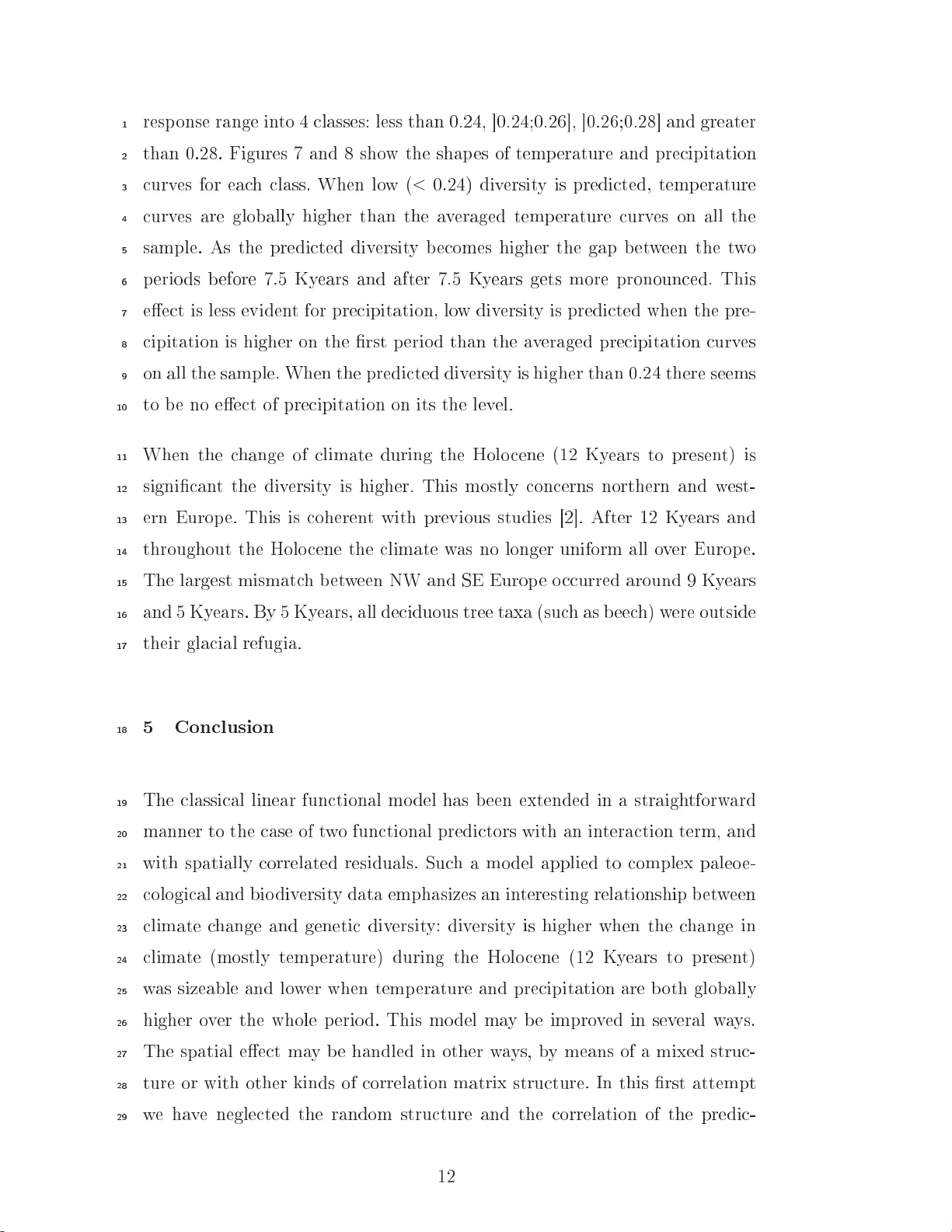
Spatio-temp oral F untional Regression on P aleo-eologial Data Liliane Bel ∗ , UMR 518 A gr oParisT e h/INRA,16, rue Claude Bernar d - 75231 Paris Ce dex 05 A vner Bar-Hen, Université R ené Des artes, MAP5, 45 rue des Saints Pèr es, 75270 Paris  e dex 06 Ra hid Cheddadi, ISEM,  ase p ostale 61, CNRS UMR 5554, 34095 Montp el lier, F r an e Rém y P etit, UMR 1202 INRA , 69 r oute d'A r  ahon 33612 Cestas Ce dex, F r an e Abstrat The inuene of limate on bio div ersit y is an imp ortan t eologial question. V ari- ous theories try to link limate  hange to alleli ri hness and therefore to predit the impat of global w arming on geneti div ersit y . W e mo del the relationship b e- t w een geneti div ersit y in the Europ ean b ee h forests and urv es of temp erature and preipitation reonstruted from p ollen databases. Our mo del links the geneti measure to the limate urv es through a linear funtional regression. The in tera- tion in limate v ariables is assumed to b e bilinear. Sine the data are georeferened, our metho dology aoun ts for the spatial dep endene among the observ ations. The pratial issues of these extensions are disussed. Key wor ds: F untional Data Analysis; Spatio-temp oral mo deling; Climate  hange; Bio div ersit y Preprin t submitted to Elsevier No v em b er 18, 2018 1 In tro dution 1 Climate reords sho w that the earth has reorded a suession of p erio ds of 2 ma jor w arming and o oling at dieren t time windo ws and sales [ 5 , 12℄. During 3 the last p ost-glaial p erio d (18000 y ears b efore the presen t), Europ e reorded 4 a 15 ◦ C to 20 ◦ C w arming dep ending on the area. A t the same p erio d there w as 5 an expansion of all forest biomes and an up w ard mo v emen t of the tree-lines 6 that rea hed an altitude 300 m higher than to da y . Although there is a w ealth 7 of paleo data and detailed limate reonstrution for the Holo ene p erio d, w e 8 still la k some kno wledge as to ho w the w arming w as reorded and what the 9 v egetation feedba ks w ere that aeted lo al or regional past limates. V arious 10 theories try to link limate  hange to alleli ri hness and therefore to predit 11 the impat of global w arming on geneti div ersit y . 12 In the reen t literature there ha v e b een a lot of theoretial results for regres- 13 sion mo dels with funtional data. Based on this framew ork, w e used a linear 14 funtional mo del to mo del the relationship b et w een geneti div ersit y in Euro- 15 p ean b ee h forests (represen ted b y a p ositiv e n um b er) and urv es of temp er- 16 ature and preipitation reonstruted from the past. The lassial funtional 17 regression mo del has b een extended in t w o w a ys to aoun t for our sp ei 18 problem. First, as the eets of temp erature and preipitation are far from 19 indep enden t w e inluded an in teration term in our mo del. This in teration 20 term app ears as a bilinear funtion of the t w o preditors. Seond, sine w e 21 ha v e spatial data there is dep endene among the observ ations. T o tak e in to 22 aoun t with dep endene the o v ariane matrix of the residuals is estimated 23 in a spatial framew ork and plugged in to generalized least-squares to estimate 24 the parameters of the mo del. The pratial diulties of these extensions will 25 b e disussed. 26 In Setion 2, w e presen t the geneti and limate data. The funtional regression 27 mo del is studied in Setion 3. Results are presen ted and disussed in Setion 4 28 ∗ Corresp onding author. Email addr ess: Liliane.Belagroparisteh.fr (Liliane Bel). 2 and onluding remarks are giv en in Setion 5. 1 2 Data 2 P ollen reords are imp ortan t pro xies for the reonstrution of limate param- 3 eters sine v ariations in the p ollen assem blages mainly resp ond to limate 4  hanges. Based on the fossil and surfae p ollen data from p ollen databases, 5 w e used mo dern analogue te hnique (MA T) to reonstrut limate v ariables. 6 Climate reonstrution is aomplished b y mat hing fossil biologial assem- 7 blages to reen tly dep osited (mo dern) p ollen assem blages for whi h limate 8 prop erties are kno wn. The relatedness of fossil and mo dern assem blages is usu- 9 ally measured using a distane metri that resales m ultidimensional sp eies 10 assem blages in to a single measure of dissimilarit y . The distane-metri metho d 11 is widely used among paleo eologists and paleo eanographers [8℄. T emp erature 12 and preipitation w ere reonstruted at 216 lo ations from the presen t ba k 13 to a v ariable date dep ending on a v ailable data. The p ollen dataset w as used 14 to reonstrut limate v ariables, throughout Europ e for the last 15 000 y ears 15 of the Quaternary . Due to the metho dology , ea h limate urv e is sampled at 16 irregular times for ea h lo ation. 17 Geneti div ersities w ere measured from v ariation at 12 p olymorphi isozyme 18 lo i in Europ ean b ee h ( F agus sylvati a L.) forests based on an extensiv e 19 sample of 389 p opulations distributed throughout the sp eies range. Based 20 on these data, v arious indies of div ersit y an b e omputed. They mainly 21  haraterize within or b et w een p opulation div ersit y . In this artile, w e fo us on 22 the H index, the probabilit y that t w o alleles sampled at random are dieren t. 23 This parameter is a go o d indiation of gene div ersit y [ 3℄. 24 The t w o datasets w ere olleted indep enden tly and their lo ations do not 25 oinide. 26 3 3 F untional Regression 1 The funtional linear regression mo del with funtional or real resp onse has 2 b een the fo us of v arious in v estigations [1, 6, 7, 11℄. W e w an t to estimate the 3 link b et w een the real random resp onse y i = d ( s i ) , the div ersit y at site s i and 4 ( θ i ( t ) , π i ( t )) t> 0 the temp erature and preipitation funtions at site s i . There 5 are t w o p oin ts to onsider for the mo deling: (i) funtional linear mo dels need 6 to b e extended to inorp orate in teration b et w een limate funtions; (ii) sine 7 w e ha v e spatial data, observ ations annot b e onsidered as indep enden t and 8 w e also need to extend funtional mo deling to aoun t for spatial orrelation. 9 W e assume that the temp erature and preipitation funtions are square in- tegrable random funtions dened on some real ompat set [0 , T ] . The v ery general mo del an b e written as: Y = f (( θ ( t ) , π ( t )) T >t> 0 ) + ε f is an unkno wn funtional from L 2 ([0 , T ]) × L 2 ([0 , T ]) to R and ε is a spatial 10 stationary random eld with orrelation funtion ρ ( . ) . 11 W e assume here that the funtional f ma y b e written as the sum of linear 12 terms in θ ( t ) and π ( t ) and a bilinear term mo deling the in teration 13 f ( θ , π ) = µ + Z [0 ,T ] A ( t ) θ ( t ) d t + Z [0 ,T ] B ( t ) π ( t ) d t + Z Z [0 ,T ] 2 C ( t, u ) θ ( t ) π ( u ) dudt = µ + h A ; θ i + h B ; π i + h C θ ; π i b y the Riesz represen tation of linear and bilinear forms. 14 A and B are in L 2 ([0 , T ]) and C is a k ernel of L 2 ([0 , T ]) . 15 Let ( e k ) k > 0 b e an orthonormal basis of L 2 ([0 , T ]) . Expanding all funtions on this basis w e get θ i ( t ) = + ∞ X k =1 α i k e k ( t ) π i ( t ) = + ∞ X k =1 β i k e k ( t ) 4 A ( t ) = + ∞ X k =1 a k e k ( t ) B ( t ) = + ∞ X k =1 b k e k ( t ) C ( t, u ) = + ∞ X k ,ℓ =1 c k ℓ e k ( t ) e ℓ ( u ) and y i = µ + + ∞ X k =1 a k α i k + + ∞ X k =1 b k β i k + + ∞ X k ,ℓ =1 c k ℓ α i k β i ℓ + ε i If the sums are trunated at k = ℓ = K the problem results in a linear 1 regression Y = µ + X φ + ε with spatially orrelated residuals with 2 X =            α 1 1 . . . α 1 K β 1 1 . . . β 1 K α 1 1 β 1 1 . . . α 1 K β 1 K . . . . . . . . . α n 1 . . . α n K β n 1 . . . β n K α n 1 β n 1 . . . α n K β n K            dim ( X ) = n × (2 K + K 2 ) o v ( ε i , ε j ) = ρ ( s i − s j ) In order to estimate the regression and the orrelation funtion parameters w e 3 pro eed b y Quasi Generalized Least Squares: a preliminary estimation of φ is 4 giv en b y Ordinary Least Squares, φ ∗ = ( X t X ) − 1 X t Y , the orrelation funtion 5 is estimated from the residuals b ε = Y − X φ ∗ and the nal estimate of φ is 6 giv en b y plugging the estimated orrelation matrix b Σ in the Generalized Least 7 Squares form ula b φ = ( X t b Σ − 1 X ) − 1 X t b Σ − 1 Y . If b oth estimations of φ and Σ are 8 on v ergen t and assuming normal distribution of the residuals then [9℄: 9 √ n ( b φ − φ ) → N (0 , lim n →∞ n ( X t Σ − 1 X ) − 1 ) The estimation of Σ is on v ergen t under mild onditions [4℄ and the on v er- 10 gene of φ is assessed for example when the funtions are expanded on a splines 11 basis [1 ℄ or on a Karh unen expansion [10℄. 12 Signiane of the preditors an b e tested if the residuals are assumed to b e 13 Gaussian, within the lassial framew ork of linear regression mo dels. 14 Sev eral parameters need to b e set. The rst  hoie is that of the orthonormal 15 5 basis. It an b e F ourier, splines, orthogonal p olynomials, w a v elets. Then the 1 order of trunation has to b e determined. The spatial orrelation funtion 2 of the residuals ma y b e of parametri form (exp onen tial, Gaussian, spherial 3 et.). These  hoies will b e made b y minimizing a ross v alidation riterion: a 4 sample with no missing data for all v ariables is determined, and for ea h site of 5 the sample a predition of the div ersit y is omputed aording to parameters 6 estimated without the site in the sample. The global riterion is the quadrati 7 mean of the predition error. 8 4 Results 9 P ollen w as olleted throughout Europ e pro viding temp oral estimation of tem- 10 p eratures and preipitation. These estimations are not regularly spaed, and 11 ha v e v ery dieren t ranges from 1 Ky ears to 15 Ky ears. Bee h geneti indies 12 are reorded in forests and do not oinide with the p ollen lo ations. Figure 13 1 sho ws the lo ations of the t w o datasets. 14 −10 0 10 20 30 40 45 50 55 60 Measurement sites pollens genetics Figure 1. Lo ations of p ollen (bla k dots) and geneti (op en irles) reords. 6 Climate v ariables are on tin uous all o v er Europ e but b ee h forests ha v e sp ei 1 lo ations. In order to mak e our data to spatially oinide, temp erature and 2 preipitation urv es are rstly estimated on a regular grid of time from 15 3 Ky ears to presen t on sites where are olleted the geneti measures. 15 Ky ears 4 orresp onds to the b eginning of migration of plan ts on to areas made free b y 5 the retreating ie sheets. 6 The in terp olation is done b y a spatio-temp oral kriging assuming the o v ariane 7 funtion is exp onen tial and separable. Figure 2 sho ws for a partiular site the 8 estimated temp erature urv e together with some neigh b oring urv es issued 9 from olleted p ollen. 10 −15000 −10000 −5000 0 −25 −20 −15 −10 −5 0 5 10 time Spatio−temporal kriging of temperature Figure 2. Resulting temp erature urv e (thi k bla k urv e) from spatio-temp oral kriging of 20 neigh b oring temp eratures urv es from reorded p ollen. W e aim to predit geneti div ersit y with preipitation and temp erature urv es. 11 This orresp onds to a funtional regression mo del with geneti div ersit y as de- 12 p enden t v ariable and temp erature and preipitation urv es as preditor v ari- 13 able. The ross v alidation riterion giv es b etter results with an expansion of 14 the preditor v ariables on a F ourier basis of order 5. Figures 3 and 4 sho w the 15 o eien t funtions A , B , and k ernel C . 16 7 −15000 −10000 −5000 0 −0.005 0.000 0.005 0.010 Function A time −15000 −10000 −5000 0 −6e−05 −4e−05 −2e−05 0e+00 2e−05 4e−05 Function B time Figure 3. Co eien t funtion A of the temp erature and o eien t funtion B of the preipitation time time Kernel C Figure 4. Kernel C of the in teration temp erature-preipitation The shap e of the o eien t funtion A sho ws that the term h A, θ i will b e 1 higher when the gap b et w een p erio ds b efore 7.5 Ky ears and after 7.5 Ky ears 2 8 is higher (temp eratures b efore 7.5 Ky ears are mostly negativ e), mean while the 1 shap e of the o eien t funtion B sho ws that the term h B , π i will b e higher 2 when the preipitation b efore 7.5 Ky ears is higher (preipitation is p ositiv e). 3 The surfae of k ernel C is ob viously not the pro dut of t w o urv es in the t w o 4 o ordinates, sho wing an eet of in teration. 5 In Figure 5 the residual v ariogram graph exhibits some spatial dep endene. An 6 exp onen tial v ariogram is tted, and the resulting o v ariane matrix is plugged 7 in to the GLS form ula to up date the o eien ts and test the eets of the 8 temp erature, preipitation and in teration. 9 0 200 400 600 800 1000 0.00030 0.00035 0.00040 0.00045 0.00050 0.00055 0.00060 Residuals variogram distance (km) semivariance nugget = 0.00037 sill = 0.00021 range = 81.5 Figure 5. Empirial and tted v ariogram on the residuals. The graphs in Figure 6 sho w that the mo del explains a part of the div ersit y 10 v ariabilit y . Ho w ev er it is far from explaining all the v ariabilit y as the R 2 is 11 equal to 0.31. 12 9 0.20 0.25 0.30 0.35 0.20 0.22 0.24 0.26 0.28 0.30 0.32 0.34 Observed response Predicted response 0.20 0.22 0.24 0.26 0.28 0.30 0.32 0.34 −0.06 −0.04 −0.02 0.00 0.02 0.04 0.06 0.08 Predicted response Residuals Figure 6. Observ ed-Predited resp onse and Predited-Residuals graphs. T able 1 giv es the analysis of v ariane of the four nested mo dels: 1 Mo del 1: E ( Y ) = µ + h A ; θ i + h B ; π i + h C θ ; π i 2 Mo del 2: E ( Y ) = µ + h A ; θ i + h B ; π i 3 Mo del 3: E ( Y ) = µ + h A ; θ i 4 Mo del 4: E ( Y ) = µ + h B ; π i 5 T able 1 Analysis of v ariane mo dels of nested mo dels The p -v alues (2.2e-16) of the tests H 0 : mo del 3 (mo del 4) against H 1 : mo del 6 2 and (1.430e-07) of the test H 0 : mo del 2 against H 1 : mo del 1 sho w that the 7 in teration and the t w o v ariables ha v e a strong eet. 8 10 −15000 −10000 −5000 0 −12 −8 −6 −4 −2 0 genetic class <0.24 years Temperature sample average class average −15000 −10000 −5000 0 −12 −8 −6 −4 −2 0 genetic class [0.24 ; 0.26[ years Temperature sample average class average −15000 −10000 −5000 0 −12 −8 −6 −4 −2 0 genetic class [0.26;0.28[ years Temperature sample average class average −15000 −10000 −5000 0 −12 −8 −6 −4 −2 0 genetic class >0.28 years Temperature sample average class average Temperature Figure 7. P attern of temp erature urv es aording to the range of the predited resp onse. −15000 −10000 −5000 0 500 600 700 800 900 genetic class <0.24 years Precipitation sample average class average −15000 −10000 −5000 0 500 600 700 800 900 genetic class [0.24 ; 0.26[ years Precipitation sample average class average −15000 −10000 −5000 0 500 600 700 800 900 genetic class [0.26;0.28[ years Precipitation sample average class average −15000 −10000 −5000 0 500 600 700 800 900 genetic class >0.28 years Precipitation sample average class average Precipitation Figure 8. P attern of preipitation urv es aording to the range of the predited resp onse. T o giv e a b etter understanding of the regression mo del w e divide the predited 1 11 resp onse range in to 4 lasses: less than 0.24, ℄0.24;0.26℄, ℄0.26;0.28℄ and greater 1 than 0.28. Figures 7 and 8 sho w the shap es of temp erature and preipitation 2 urv es for ea h lass. When lo w ( < 0.24) div ersit y is predited, temp erature 3 urv es are globally higher than the a v eraged temp erature urv es on all the 4 sample. As the predited div ersit y b eomes higher the gap b et w een the t w o 5 p erio ds b efore 7.5 Ky ears and after 7.5 Ky ears gets more pronouned. This 6 eet is less eviden t for preipitation, lo w div ersit y is predited when the pre- 7 ipitation is higher on the rst p erio d than the a v eraged preipitation urv es 8 on all the sample. When the predited div ersit y is higher than 0.24 there seems 9 to b e no eet of preipitation on its the lev el. 10 When the  hange of limate during the Holo ene (12 Ky ears to presen t) is 11 signian t the div ersit y is higher. This mostly onerns northern and w est- 12 ern Europ e. This is oheren t with previous studies [ 2℄. After 12 Ky ears and 13 throughout the Holo ene the limate w as no longer uniform all o v er Europ e. 14 The largest mismat h b et w een NW and SE Europ e o urred around 9 Ky ears 15 and 5 Ky ears. By 5 Ky ears, all deiduous tree taxa (su h as b ee h) w ere outside 16 their glaial refugia. 17 5 Conlusion 18 The lassial linear funtional mo del has b een extended in a straigh tforw ard 19 manner to the ase of t w o funtional preditors with an in teration term, and 20 with spatially orrelated residuals. Su h a mo del applied to omplex paleo e- 21 ologial and bio div ersit y data emphasizes an in teresting relationship b et w een 22 limate  hange and geneti div ersit y: div ersit y is higher when the  hange in 23 limate (mostly temp erature) during the Holo ene (12 Ky ears to presen t) 24 w as sizeable and lo w er when temp erature and preipitation are b oth globally 25 higher o v er the whole p erio d. This mo del ma y b e impro v ed in sev eral w a ys. 26 The spatial eet ma y b e handled in other w a ys, b y means of a mixed stru- 27 ture or with other kinds of orrelation matrix struture. In this rst attempt 28 w e ha v e negleted the random struture and the orrelation of the predi- 29 12 tors. T aking in to aoun t these t w o  harateristis should giv e a b etter w a y 1 to understand the real eet of limate on bio div ersit y . 2 13 Referenes 1 [1℄ H. Cardot, F. F errat y , P . Sarda, F untional linear mo del, Statist. Probab. 2 Lett. 45 (1999) 11-22. 3 [2℄ R. Cheddadi, A. Bar-Hen, Spatial gradien t of temp erature and p oten tial 4 v egetation feedba k aross Europ e during the late Quaternary , Climate 5 Dynamis (in press). 6 [3℄ B. Comps, D. Gömöry , J. Letouzey , B. Thiébaut, R.J. P etit, Div erging 7 trends b et w een heterozygosit y and alleli ri hness during p ostglaial ol- 8 onization in the Europ ean b ee h, Genetis 157(2001) 389-397. 9 [4℄ N. Cressie, Statistis for spatial data, Revised Edition, Wiley , New-Y ork, 10 1993 11 [5℄ D. Dahl-Jensen, K. Mosegaard, N. Gundestrup, G.D. Clo w, S.J. Johnsen, 12 A.W. Hansen, N. Balling, P ast T emp eratures Diretly from the Greenland 13 Ie Sheet, Siene 282 (1998) 268-271. 14 [6℄ J. F an, J.T. Zhang, T w o-step estimation of funtional linear mo dels with 15 appliation to longitudinal data. J. R. Stat. So . Ser. B Stat. Metho dol. 16 62 (2000) 303-322. 17 [7℄ J.J. F ara w a y , Regression analysis for a funtional resp onse, T e hnometris 18 39 (1997) 254-261. 19 [8℄ J. Guiot, Metho dology of the last limati yle reonstrution in F rane 20 from p ollen data, P alaeogeograph y P alaeo limatology P alaeo-eology 80 21 (1990) 49-69. 22 [9℄ X. Guy on, Statistique et éonométrie, Ellipses Mark eting, P aris, 2001 23 [10℄ H.G. Müller, U. Stadtm üller, Generalized funtional linear mo dels, Ann. 24 Stat. 33 (2005) 774-806 25 [11℄ J.O. Ramsa y , B.W. Silv erman, F untional Data Analysis, Springer, New- 26 Y ork, 1997 27 [12℄ J. Seierstad, A. Nesje, S.O. Dahl, J.R. Simonsen, Holo ene glaier u- 28 tuations of Gro v abreen and Holo ene sno w-a v alan he ativit y reon- 29 struted from lak e sedimen ts in Groningstolsv atnet, w estern Norw a y , The 30 Holo ene 12:2 (2002) 211-222. 199 14