A Dynamic Programming Approach To Length-Limited Huffman Coding

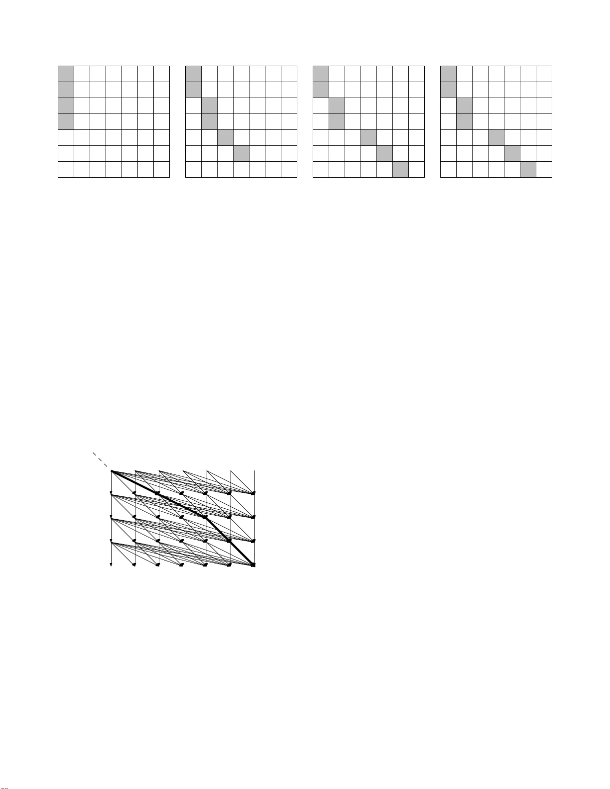
1 A Dynamic Programming App roach T o Length-Limited Huf fman Coding Mordecai Golin, Member , I EEE, and Y an Zhan g Abstract —The “state-of-the-art” in Length Limited Huffman Coding algorithms is the Θ( N D ) -ti me, Θ( N ) -space one of Hirschberg and Larmore, where D ≤ N is the length restriction on the code. This is a very clev er , very problem specific, technique. In this note we show that there is a simple Dynamic-Programming (DP) method that solves t h e problem with the same t i me and space bounds. The fact that ther e was an Θ( N D ) ti me DP algorithm was pre viously known; it is a straig htforwar d DP with t h e Monge p roperty (which p ermits an order of magnitud e speedup). It was not interesting, though, because it also required Θ( N D ) space. The main result of th is paper is the technique dev eloped for reducing the space. It is quite simple and applicable to many other problems modeled by DPs with the Monge property . W e illustrate this with examples from web-p roxy design and w i reless mobile p aging. Index T erms —Prefix-Fr ee Codes, Hu ffman Coding, Dynamic Progra mming, W eb-P roxies, Wir eless Paging, the Monge prop- erty . I . I N T RO D U C T I O N O ptimal pr efix-free co ding, or Huffman codin g , is a stan- dard co mpression techniq ue. Giv en an encoding alph a- bet Σ = { σ 1 , . . . , σ r } , a cod e is just a set of words in Σ ∗ . Giv en n pro babilities or nonnegativ e freque ncies { p i : 1 ≤ i ≤ n } , and associated code { w 1 , w 2 , . . . , w n } the cost of the code is P n i =1 p i | w i | where | w i | den otes the length of w i . A co de is pr e fix-fr ee if n o codeword w i is a prefix of any other co dew ord w j . An optima l prefix- free c ode f or { p i : 1 ≤ i ≤ n } is a prefix-fr ee code that minimizes its cost among all prefix- free codes. In [1], Huffman ga ve the now classical O ( n log n ) time algorithm fo r solving this problem . If the p i ’ s are g i ven in sorted ord er , Huffman’ s algorithm can be improved to O ( n ) time [2]. I n this note we will always a ssume that th e p i ’ s are presorted and that p 1 ≤ p 2 ≤ . . . ≤ p n . In som e applicatio ns, it is desirable that th e length of all code words are bound ed by a con stant, i.e. , | w i | ≤ D where D is giv en. Th e prob lem of finding the minimal cost prefix - free code among all codes satisfying this length con straint is the length-limited Huffman coding (LLHC) pro blem, wh ich we will consider h ere. Fig. 1 g iv es an examp le of inpu ts for which the Hu ffman code is no t the same as th e length-limited Huffman cod e. The fir st alg orithm fo r LL HC was due to Ka rp [ 3] in 19 61; his a lgorithm is based o n integer linear prog ramming (IL P), M. Golin and Y . Zhang are with the Department of Computer Science & Engineeri ng, Hong Kong UST , ClearW at er Ba y , Ko wloon, Hong K ong. T heir research was parti ally supported by HK RGC CERG grants HKUST 6312/04E and 613105. which, using standard ILP solving techniques, leads to an exponential time algo rithm. Gilbert [4] in 1 971 was interested in this problem becau se of th e issue of inaccur ately kn own sources; since the p robabilities p i ’ s are no t known precisely , a set of codes with limited length will, in some sense, be “safe”. The algorithm p resented in [4] was an enum eration one and therefor e also runs in expone ntial time. In 1972 Hu and T an [ 5] d ev eloped an O ( nD 2 D ) time Dyna mic Program ming (DP) algorithm. T he first polynom ial time algorithm, runnin g in O ( n 2 D ) time and using O ( n 2 D ) space, was p resented by Garey in 19 74 [6]. Garey’ s alg orithm was based on a DP formu lation similar to th at developed by Knu th fo r deriving optimal bin ary search tre es in [7] a nd h ence only works for binary e ncoding alphabets. A decade later , Larmor e [8] gave an algorithm ru nning in O ( n 3 / 2 D log 1 / 2 n ) time a nd using O ( n 3 / 2 D log − 1 / 2 n ) sp ace. Th is algo rithm is a hyb rid of [ 5] and [6], and there fore also on ly works fo r th e binary ca se. This was finally improved by Larmore and Hirschbe rg [9 ] who gave a totally different algo rithm running in O ( nD ) time and using O ( n ) space. In that paper , the authors fir st tra nsform th e length-limited Huffman coding p roblem to th e Coin Collec- tor’ s proble m, a special ty pe of Knapsack problem , an d then , solve the Co in Collecto r’ s p roblem by what they n ame the P ac kage-Mer ge algorithm. Their result is a very clever sp ecial case algorithm developed for th is specific prob lem. Theoretically , Larmor e and Hirschb erg’ s result was later superseded for the case 1 D = ω (log n ) by two alg orithms based on the p arametric sear ch p aradigm [10]. The algo- rithm by Agg arwal, Schieb er and T okuyama [11] runs in O ( n √ D log n + n log n ) time and O ( n ) space. A later im- provement by Schieb er [12] runs in n 2 O  √ log D log log n  time and uses O ( n ) space. These algor ithms are very complicated , though , and e ven for D = ω (log n ) , the Larmore-Hir schberg one is th e one used in pr actice [1 3], [14]. For completen ess, we point out th at the algorithm s of [9], [1 1], [12] are a ll o nly claimed for the binary ( r = 2 ) case but they can be exten ded to work for the non-b inary ( r > 2) case u sing observations similar to those we provide in Ap pendix A for th e deriv atio n of a DP for the generic r -ary LLHC pr oblem. Shortly af ter [ 9] app eared, Larm ore and Przytycka [15], [16], in the co ntext o f par allel progra mming, g av e a simp le dynamic pr ogramm ing formulation for the bin ary Huffman coding pro blem. Although their DP was for regular Huffman coding and not the LL HC pro blem, we will see that it is quite easy to modify their DP t o model the LLHC problem. It is then straightfor ward to show that their for mulation also perm its 1 f ( n ) = ω ( g ( n )) if ∃ N, c > 0 such that ∀ n > N , f ( n ) ≥ g ( n ) . 2 constructing th e optimal tree in Θ( nD ) time b y co nstructing a size Θ( nD ) DP table. This is don e is Section II. This straight DP appr oach would not be as goo d as the Larmore - Hirschberg on e, though , because, like many DP algorithms, it requires maintaining the entire DP table to permit backtr acking to constru ct the solutio n, wh ich would r equire Θ( nD ) space. The m ain resu lt of this no te is the d ev elopmen t of a simple technique (sectio n I II) that permits red ucing the DP space consump tion down to O ( n ) , thus match ing the Larmo re- Hirschberg performance with a straightforward DP model. Our technique is not restricted to L ength-Lim ited codin g. It can be used to reduce space from O ( nD ) to O ( n + D ) in a variety o f O ( nD ) time DPs in the literatur e. In Sectio n IV we illustrate with examples from th e D-median on a line pro blem ( placing web p roxies on a linea r top ology network) [17] and wireless paging [18]. I I . T H E D Y N A M I C P RO G R A M M I N G F O R M U L AT I O N Set S 0 = 0 and S m = P m i =1 p i for 1 ≤ m ≤ n . Larmore and Przytycka [ 16] fo rmulated the bin ary Huffman cod ing problem as a DP (1) wher e H (0) = 0 and for 0 < i < n : H ( i ) = min max { 0 , 2 i − n }≤ j 0 , 0 ≤ i < n (2) where H ( D , n − 1) will den ote the cost of th e optimal length - limited Huffman code and c ( d ) i,j =    0 i = j = 0 S 2 i − j max { 0 , 2 i − n } ≤ j < i ∞ otherwise. (3) In the next subsection we will see an inter pretation of th is DP (which also provid es an interpretation of (1)). In order to make this note self-con tained, a co mplete deriv ation o f the DP for the r -ary alphab et case is p rovided in Appen dix A. As far as ru nning time is con cerned, (1) appear s to a- priori requ ire O ( n 2 ) time to fill in its co rrespond ing DP table. [16] used the inhe rent co ncavity of S m to reduce this time down to O ( n ) by transfo rming th e problem to an instance of the Con cav e Least W eight Subsequen ce (CL WS) p roblem and using on e o f the known O ( n ) time algorith ms, e.g., [20], for solving that proble m. Similarly , (2) appears to a-prior i r equire Θ( n 2 D ) time to fill in its DP table. W e will see that we may again use the conc avity of S m to redu ce this down by an o rder of magnitud e, to O ( nD ) by using the SMA WK algorithm [2 1] for find ing row-minima of matrices a s a subr outine. Unlike the CL WS algorithm s, the SMA WK o ne is very simp le to cod e and very efficient imp lementations are available in different packages, e. g., [22], [23]. In the co nclusion to this note, after the ap plication o f the techniq ue beco mes un derstandab le, we will e xplain why [16] n eeded to use the mo re comp licated CL WS rou tine to so lve the basic DP while we c an use th e simpler SMA W K one. The O ( nD ) DP algor ithm for solving the LL CH prob lem, while seemingly never explicitly stated in the literature , was known as folklore. Even though it is much simpler to imple- ment than the O ( nD ) Larmor e and Hirsch berg [9] Package- Merge algorithm it suf f ers from the drawback of requiring Θ( nD ) space. The main contribution o f this note is th e observation that its spac e ca n be red uced d own to O ( n + D ) making it com parable with Package-Merge. Note that since, for the LLHC problem we may trivially assume D ≤ n , th is implies a space require ment o f O ( n ) . Further more, our space improvement will work not only for the LLHC problem b ut for all DPs in form (2) where the c ( d ) i,j satisfy a particu lar property . A. The meanin g of The DP W e quickly sketch the m eaning of the DP (2) for th e binary case. Figure s 1 and 2 illustrate this sketch. W e n ote that in or der to stress the parts im portant to our analysis, our for malism is a bit different than [16], [ 19]. A c omplete deriv ation of the DP fo r the r -ary ca se with the app ropriate general versions of the lem mas and observations stated below along with their proof s, is pr ovided in Appen dix A. It is stand ard th at th ere is a 1 − 1 cor respond ence between binary prefix-fr ee code with n words and binary tree with n leav es. T he set of edges from a n internal node to its children are labeled by a 0 or 1 . Eac h leaf correspo nds to a code word, which is th e conc atenation of the character s o n th e roo t-to- leaf path. Th e cost of the code eq uals the weig h ted external path length of the tre e. So we are r eally interested in fin ding a binary tree with minimu m weigh ted external path leng th. Denote th e heig ht of the tree by h. T he bottommo st leaves are on level 0 ; the r oot on lev el h . Optimal assignmen ts o f the p i ’ s to the leaves alw ays assign smaller valued p i ’ s to lea ves at lower levels. A node in a b inary tree is co mplete if it has two child ren and a tree is complete if a ll of its intern al nodes are complete. A min-co st tree must b e comple te, so we restrict ourselves to complete trees. A c omplete tree T of height h can be completely represented by a sequen ce ( i 0 , i 1 , . . . , i h ) , where i k denotes the num ber of in ternal no des at lev els ≤ k . Note th at, by definition, i 0 = 0 , i h = n − 1 . Also note th at e very level must contain at least on e intern al node so i 0 < i 1 < · · · < i h . Finally , it is straightfor ward (see App endix A) to show that the to tal number of lea ves o n level < k is 2 i k − i k − 1 , so 2 i k − i k − 1 ≤ n fo r all k . For techn ical r easons, becau se we will be dealing with trees having height at most h ( but not n ecessarily equ al to h ), we allow initial pad ding of the sequence by 0 s so a sequence repr esenting a tree will be o f the form ( i 0 , i 1 , . . . , i h ) that has the following pr operties Definition 1: Sequ ence ( i 0 , i 1 , . . . , i h ) is valid if • ∃ t > 0 such tha t i 0 = i 1 = · · · = i t = 0 , • 0 < i t +1 < i t +2 < · · · < i h ≤ n − 1 • 2 i k − i k − 1 ≤ n fo r all 1 ≤ k ≤ h . 3 p 1 p 2 p 3 p 4 p 5 p 6 p 7 k i k 2 i k − i k − 1 0 1 2 3 4 5 0 1 3 4 5 6 2 5 5 6 7 p 1 p 2 p 3 p 4 p 5 p 6 p 7 k i k 2 i k − i k − 1 0 1 2 3 4 0 2 4 5 6 4 6 6 7 Co de[1] = 00000 Co de[2] = 00001 Co de[3] = 0001 Co de[4] = 0010 Co de[5] = 0011 Co de[6] = 01 Co de[7] = 1 Co de[1] = 0000 Co de[2] = 0001 Co de[3] = 0010 Co de[4] = 0011 Co de[5] = 010 Co de[6] = 011 Co de[7] = 1 0 1 0 0 0 0 0 1 1 1 1 1 0 1 0 0 0 0 0 1 1 1 1 1 Fig. 1. T wo trees and their correspo nding sequence s I and codes. The left tree has sequence I 1 = (0 , 1 , 3 , 4 , 5 , 6) . The right tree has sequence I 2 = (0 , 2 , 4 , 5 , 6) . Note that, for both trees, 2 i k − i k − 1 is the number of le av es belo w le vel k . For input frequenc ies ( p 1 , . . . , p 7 ) = (1 , 1 , 2 , 2 , 2 , 4 , 5 , 9) . The left tree is an optimal Huffma n code while the right tree is an optimal length -limited Huffman code for D = 4 . Note t hat we allo w padding seque nces with initia l 0 s, so the right tree could also be represent ed by seque nces (0 , 0 , 2 , 4 , 5 , 6) , (0 , 0 , 0 , 2 , 4 , 5 , 6) , etc.. 0 0 0 0 0 ∞ ∞ ∞ ∞ ∞ ∞ ∞ ∞ ∞ ∞ 2 2 2 2 6 6 6 6 13 10 10 10 19 18 18 35 32 31 57 54 0 0 0 0 – – – – 0 0 0 0 0 1 1 1 0 1 1 1 2 3 3 3 4 4 5 5 H ( d, i ) J ( d, i ) d i 0 1 2 3 4 0 1 2 3 4 5 6 d i 0 1 2 3 4 0 1 2 3 4 5 6 Fig. 2. Solving the DP in equati on 2 for ( p 1 , . . . , p 7 ) = (1 , 1 , 2 , 2 , 2 , 4 , 5 , 9) with D = 4 . H ( d, i ) is the valu e defined by (2); J ( d, i ) is the inde x j for which the v alue H ( d, i ) in (2) is achie ved. The circl ed entries yield the seque nce (0 , 2 , 4 , 5 , 6) (th e 6 comes from the fact that we are calcula ting H (4 , 6 ) ) which is e xactly the sequence I 2 from Figure 1. T he righth and tree in Figure 1 is therefore an optimal lengt h-limite d Huffman code for D = 4 . A sequence is complete if it is valid and i h = n − 1 . W e can rewrite the c ost function for a tree in terms of its complete sequence. Lemma 1: If complete seq uence ( i 0 , i 1 , . . . , i h ) represen ts a tree, then the cost of the tree is P h k =1 S 2 i k − i k − 1 . (Note that padding complete sequen ces with initial 0 s d oes not change the cost of the sequen ce.) W e may mechan ically extend th is cost fu nction to all valid sequences as follows. Definition 2: For valid I = ( i 0 , i 1 , . . . , i h ) , set cost ( I ) = h X k =1 S 2 i k − i k − 1 . I is optimal if cost ( I ) = min I ′ cost ( I ′ ) wh ere the minimum is taken over all len gth h sequen ces I ′ = ( i ′ 0 , i ′ 1 , . . . , i ′ h ) with i ′ h = i h , i.e., all sequenc es o f the same length that end with the same value. Our g oal is to find op timal trees b y usin g the DP to optimize over valid sequences. An imm ediate issue is that no t all complete seq uences represent trees, e.g., I = (0 , 3 , 4 , 5) is complete fo r n = 6 but, by observation, d oes not represent a tree. Th e saving fact is tha t even th ough not all complete sequences represent tr ees, all optimal complete sequen ces represent trees. Lemma 2: An o ptimal valid sequence en ding in i h = n − 1 always rep resents a tree. Thus, to solve th e LLH C prob lem of finding an optimal tree of heig ht ≤ D , we only n eed to find an optimal valid seque nce of length h = D end ing with i D = n − 1 (reconstructin g the tree f rom the sequenc e can be done in O ( n ) time). In the DP defined by equation s (2) and ( 3), H ( d, j ) clearly models the recurr ence for findin g an o ptimal valid sequen ce ( i 0 , i 1 , . . . , i d ) of len gth d with i d = j so this D P solves the problem . Note that, a-p riori, filling in th e DP table H ( · , · ) one 4 entry a t a time seems to requ ire O ( n 2 D ) time. W e will now sketch the standard way of reducing this time down to O ( nD ) . Befor e do ing so we mu st disting uish b etween the value pr oblem and th e construction pr o blem . The value problem would be to calculate the value of H ( D , n − 1) . The co nstruction p roblem would be to con struct an optimal valid sequ ence I = ( I 1 , I 2 , . . . , I D ) with I D = n − 1 and cost ( I ) = H ( D , n − 1) . This would requ ire backtrack ing throug h the DP table b y setting I 0 = 0 , I D = n − 1 and finding I 1 , I 2 , . . . I D − 1 such that ∀ 0 < d ≤ D , H ( d, I d ) = H ( d − 1 , I d − 1 ) + c ( d ) I d ,I d − 1 . (4) B. Solvin g the V alue pr oble m in O ( nD ) time Definition 3: An n × m matrix M is Monge 2 if for 0 ≤ i < n − 1 and 0 ≤ j < m − 1 M i,j + M i +1 ,j +1 ≤ M i +1 ,j + M i,j +1 (5) The Monge pro perty can be thought o f as a discrete version of concavity . It appears implicitly in many optimization problem s for which it perm its speeding up their solutions ([24]) provides a nice survey). One of th e classic techniques u sed is the SMA W K algorithm for finding row-minima. Giv en an n × m matrix M , th e minimu m of r ow i , i = 1 , . . . , n is the entry of r ow i that has the smallest value; in case of ties, w e take the rig htmost entry . Thus, a solutio n of the row-minima problem is a collection of indices j ( i ) , i = 1 , . . . , n su ch that M i,j ( i ) = min 0 ≤ j