Covariance of centered distributions on manifold

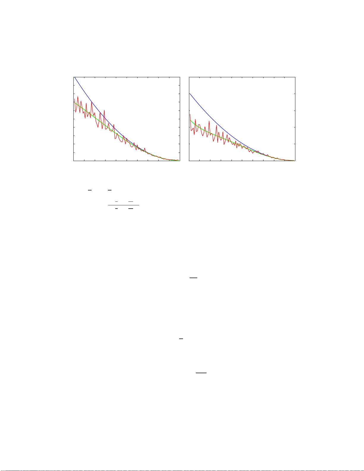
Co v ariance of cen tered distributions on manifold Nik ola y H. Balo v ∗ balov@st at.fsu.e du August 29, 2021 Abstract W e define and study a f amily of distributions with domain com- plete Riemannian manifold. They are o btained by pro jection onto a fixed tangen t space via the inv erse exp on ential map. Th is construction is a p opular c hoice in the literature for it mak es it easy to generalize w ell kno wn multiv ariate Euclidean distributions. Ho wev er, most of the a v ailable solutions use co ordinate sp ecific definition th at mak es them less v ersatile. W e defin e the distributions of int erest in co ord inate in- dep end en t w a y by utilizing co-v arian t 2-t ensors. Then w e stud y the relation of th ese distributions to their Euclidean counterparts. In par- ticular, w e are interested in relating the co v ariance to the tensor that con trols distribution concen tration. W e find app ro ximating expres- sion for this r elation in general and giv e more precise formulas in case of manif olds of constant cu rv atur e, p ositiv e o r negativ e. Results are confirmed by sim ulation studies o f the standard normal distrib u tion on the un it-sphere and h yp erb olic plane. 1 In tro duction W e ar e interes ted in defining and studying some of the prop erties of dis- tributions on complete Riemannian manifolds. A typical example of such manifolds is the unit n-sphere S n . In this sense, the sub ject of our study has ∗ Florida State Universit y , Depar tmen t of Statistics 1 as a primary application, but not limited to, directional statistics, a branch of statistics dealing with directions and ro tations in R n . Pioneers in the field are Fisher, R.A., [6] a nd v on Mises. In recen t y ears directional statistics pro v ed to b e useful in v ariet y of discipline s lik e shap e analysis [9], geology , crystallography [8], bioinformatics [11] and da t a mining [2]. The b est kno wn distribution from the field o f directional statistics is the v on Mises-Fisher distribution. It is defined on the unit n-sphere by the densit y f n ( x ; µ, k ) = C n ( k ) exp( k µ ′ x ) , x ∈ S n , where k ≥ 0, µ ∈ S n and normalizing constan t C n ( k ). It is applied initially for studying electric fields (n=2). Its one dimensional v a rian t, t he v on Mises distribution, is also known as the circular normal distribution. Another imp orta nt distribution is Fisher-Bingham-Ken t(FBK) distribu- tion, prop osed b y Ken t, J. in 1982. It is defined on S 2 b y the densit y f ( x ) = 1 c( κ, β ) exp { κ γ 1 · x + β [( γ 2 · x ) 2 − ( γ 3 · x ) 2 ] } , where γ 1 , γ 2 and γ 3 are t hree orhonor mal disrections in R 3 . A recen t a ppli- cation of Kent distribution can b e found in [7]. The family of cen tered distributions w e are going to consider includes v on Mises-Fisher distributions but not FBK distributions whic h are of mixed nature. Cen tered distributions are obtained by pro jecting the distribution domain onto a fixed v ector space, namely a t a ngen t space on manifold. This approac h is w ell kno wn and easy t o implemen t. Ho w ev er, w e think tha t not a ll of its asp ects ar e tr eat ed rigorously . One problem that needs care is defining distributions in coordinate free manner. This issue is impo rtan t when the domain is a compact Riemannian manifold as S n and do es not accept a global parametrization. Another problem arises in the study o f co v aria nce, whic h has co o rdinate sp ecific nature. Only those prop erties of distributions that a re co ordinate system in v aria n t a r e relev an t in comparison studies. Here w e do not t arget a sp ecific application, but rather aim at generaliza- tion and p edagogical impro v emen t o ve r the exis ting solutions lik e provid ing co ordinate free definition of la r ge class of distributions on complete mani- folds. Another direction in this study is the impact o f domain curv ature o n the cov ariance of distributions of in terest. Again, we impro v e up on some 2 existing results [12], b y g eneralizing and b eing more precise . Finally , we pro vide simulation results, something t hat up to our know ledge is missing in the literature, that illustrate and confirm the fo r ma l dev elopmen ts on sp ecific spaces of constan t curv ature, the unit 2-sphere and hyperb olic plane. 2 Definiti o n of cen tered distri butions Let M b e a Riemannian n-manifold, q ∈ M and let E xp q b e the exp onen- tial map a t q , E xp q : T q M → M . If M is complete, then the exp onential map E xp q is defined on the whole tangen t space T q M . Throughout this pap er w e will assume that M is a complete Riemannian n-manifold. There is a maximal op en set B ( q ) in T p M con taining the origin, where E xp q is a diffeomorphism. Then the set B ( q ) = E xp q ( B ( q )) is called maximal normal neighborho o d of q . On this normal neigh b orho o d the exp onen tial map is inv ertible and let Log q = E xp − 1 q : B ( q ) → T p M b e its inv erse, the so called log-map. Log q is diffeomorphism on B ( q ). The Borel sets on M ge nerated b y the op en s ets on M fo rm a σ -a lgebra A on M. An y Riemannian manifold has a nat ura l measure V on A , called volume me asur e . In lo cal co ordinates x it is giv en by dV ( x ) = p | G ( x ) | dx, where G ( x ) is the matrix repres entation of the metric tensor, | G | is its de- terminan t and dx is the Leb esgue measure in R n . More details one can find in [4], c h. 3.3. W e consider a family Q of distributions on M given by densit y differen tials dQ ( p ; q , T , f ) = k f ( T ( L og q p, Log q p )) dV ( p ) , (1) where q ∈ M , T is a symmetric and p ositiv e definite co-v ariant 2-tensor (bi- linear form) at tangen t space T q M , f : R → R + is a function on M and k is a normalizing constan t. W e call the elemen ts of Q c enter e d distributions for an obv ious reason - their densities are defined via pro jection on to a single tangen t space ( T q M ) placed at a cen t r al p oint ( q ). Note that their intrinsic means ma y o r may not coincide with q . Als o, as defined the distributions from Q are absolute con tin uous with resp ect to the volume measure with k f ( T ( ., . )) b eing their densities . 3 A particular mem b er of the fa mily Q tak es T ( X , Y ) = < X , Y >, X , Y ∈ T q M , f ( t ) = exp( − 1 2 σ 2 t ) , and defines the so called standar d normal distribution on M at q . Sometimes w e w an t the log -map to b e surjectiv e on the en tire tang ent space at q except ev en tually a subset of measure zero. With the curren t definition of the log- map w e hav e Log q ( B ( q )) = B ( q ) and when the cut lo cus C u t ( q ) of q is non- empt y , B ( q ) is a b ounded star-lik e neigh b orho o d in T p M . Can w e extend the definition of Log q so that it cov ers the maximal p ossible image of B ( q ), T q M ? W e a r e go ing to in tro duce a m ulti-v alue v ersion of the log-map designed to meet this requiremen t. The set of critical p oints of E xp q , i.e. the set where E xp q is not diffeo- morphism, is closed and with v olume measure zero. (for more details see [4], Th 3.2 and Prop. 3.1). In fact, the set of no n- critical p oints of E xp q is exactly B ( q ), the maximal nor mal neigh b orho o d of q . T hus , w e hav e that B ( q ) is op en in M and V ( M \B ( q )) = 0. F or an y p ∈ B ( q ), there exists a neigh b orho o d V of p such that V ⊂ B ( q ). Since W = E xp − 1 q ( V ) is op en in T p M , whic h has a coun table basis , W has coun tably man y connecte d com- p onen ts, W = ∪ i ≥ 1 W i . Moreo v er, each connected comp o nent W i of W maps diffeomorphically on V by E xp q . Therefore, if we consider B ( q ) to b e a submanifold of M, then the map E xp q : E xp − 1 q ( B ( q )) → B ( q ) , is a co v ering of B ( q ). In fact, w e can tak e V = B ( q ) and then E xp q | W i : W i → B ( q ) are diffeomorphisms. Define Log q | W i ( p ) = v i , for the uniq ue v i ∈ W i suc h that E xp q ( v i ) = p . The diffeomorphisms Log q | W i : B ( q ) → W i w e call le afs of the log- map. The m ulti-v a lue v ersion ] Log q of Log q is defined on the entire B ( q ) by ^ Log q p = { Log q | W i ( p ) } i ≥ 1 , p ∈ B ( q ) . (2) W e define f ( T ( ^ Log q p, ^ Log q p )) = ∞ X i =1 f ( T ( Log q p | W i , Log q p | W i )) . (3) 4 and then the distribution form (1) has to b e read as dQ ( p ; q , T , f ) = k f ( T ( ^ Log q p, ^ Log q p )) dV ( p ) = k ∞ X i =1 f ( T ( Log q p | W i , Log q p | W i )) dV ( p ) . W e refer to the op eration (3) as folding a densit y . Basically , the support of f determines ho w man y leafs of the log- map w e use. Recall that if ( x 1 , ..., x n ) is an orthonormal basis of T q M , the normal co ordinate system on W i is giv en b y v = ( v 1 , ..., v n ) 7→ φ ( v ) = E xp q ( v 1 x 1 + ... + v n x n ) , v 1 x 1 + ... + v n x n ∈ W i and the log-map is particularly simple, Log q | W i ( v ) ≡ Log q φ ( v ) | W i = v . The b enefit of introducing (2) and (3) is clear when one integrates func- tions of the log-map. F or example, exp ectatio n with resp ect to Q ∈ Q o f an y measurable function h ( p ) o n M is E h = k X i Z M h ( p ) f ( T ( Log q p | W i , Log q p | W i )) dV ( p ) = k X i Z φ − 1 ( W i ) h ( φ ( v )) f ( T ( v , v )) dV ( φ ( v )) = Z R n h ( φ ( v )) f ( T ( v , v )) dV ( φ ( v )) , where the last in tegral is the Lebesgue one on the whole R n . Using the m ulti-v a lue log-map all densit y functions f in R n , like the norma l ones, can b e manipulated easier on a general manifold M, b ecause we do not c hange their supp ort. Example 1 L et M , b e the unit n-s pher e S n . Fix a p oint q ∈ S n . The cut lo cus p oint for q is − q , the antip o dal p oint. Thus, B ( q ) = S n \{− q } . Define U k = B k π ( q ) , the b al l on T p S n with r adius k π , k ≥ 1 . The maximal normal neighb orho o d for q is U 1 . We have E xp − 1 q ( B ( q )) = ∪ i W i for W i = B ( i +1) π ( q ) \ B iπ ( q ) . L et n q p = Log q p/ || Log q p || b e the unit tangent ve ctor at q in the d ir e ction of p, then Log q | B 1 ( p ) = d ( q , p ) n q p for d ( q , p ) = cos − 1 < q , p > ∈ [0 , π ] and ^ Log q p = { ( d ( q , p ) ± 2 π i ) n q p } i ≥ 0 . 5 Remark 1 I n a sense, the pr op ose d extension o f the lo g-ma p with c orr e- sp ond i n g mo difie d d i s tributions ( 3 ) is gen e r alization of the c onc ept of wr a pp e d distributions. These ar e den s ities f o n the line, ’wr app e d’ ar ound the cir cum- fer enc e of the unit cir cle S 1 : f ( θ ) = P ∞ i = −∞ f ( θ + 2 π i ) , θ ∈ [0 , 2 π ) , as use d in [2]. Example 2 V on Mises-Fisher distribution is a c enter e d distribution of fo rm (1) if we take q = µ , T ( v , v ) = v ′ v = || v || 2 , f ( t ) = c 0 exp( k cos ( t )) , t ∈ [0 , 2 π ] and a norm a lizing c onstant c 0 . Supp ort of f is b ounde d and we use only the first le af of the lo g- map. Example 3 Gamma distribution on M c an b e de fi ne d by f ( t ) = c 0 t k − 1 exp( − t/θ ) , t ≥ 0 for θ > 0 and T ( v , v ) = v ′ v . Con s tant c 0 is determine d by c − 1 0 = Z R n | v | k − 1 exp( −| v | /θ ) dv = Z ∞ 0 ( Z S n r dφ ) r k − 1 exp( − r ) dr = 2 π ( n +1) / 2 θ n + k Γ( n + k ) Γ(( n + 1) / 2) , wher e we use d that the a r e a of S n r is 2 π ( n +1) / 2 r n Γ(( n +1) / 2) . Be c ause the supp ort o f f is the whole R , we h a ve a folde d density. Unfortunately , b o th von Mises-Fisher and Gamma multiv ariate distribu- tions do not hav e explicit expression for their second moments whic h mak e them less useful in the con text of the follo wing results. 3 Appro ximating the co v ariance Let Q b e a distribution from Q . Co v ariance of Q w e call a contra-v ariant 2-tensor at tangen t space T q M given by Σ = k Z p ( Log q p )( Log q p ) ′ f ( T ( Log q p, Log q p )) dV ( p ) . Note that when q is the mean (in trinsic) of Q , Σ is a cov ariance in the usual sens e, but here w e do not require q to be a mean and w e use the 6 term co v ariance in a differen t context, namely , as a quan t it y measuring the disp ersion ab out the cen ter q of Q . W e w ant to obtain an a pproximating expression for the co v ar ia nce of Q as a function o f the tensor T and the first few momen ts o f f. In normal co ordina t es v at q , the volume measure can b e approx imated b y dV ( v ) = [1 − 1 6 v ′ ( Ric ) v + O ( | v | 3 )] dv , (4) where Ric is the ma t rix represen tation of the Ricci tensor (see for example Th. 2.1 7 in Cha v el [4]). X. P ennec [12] used equation (4) to appro ximate the co v ariance of norma l distribution. His appro ximation is Σ ≈ T − 1 − 1 3 T − 1 ( Ric ) T − 1 . W e use the ab ov e approx imation of the volume form to o btain more gen- eral result applied fo r densities of cen tered distributions giv en b y (1). In addition, w e deriv e more precise v ariance estimation on the unit 2 -sphere and the h yp erplane. Finally , w e provide some simulation results to confirm the formulas . Let T b e the mat r ix represen tation of tensor T with resp ect to co ordinates v . Let T − 1 = U Λ U ′ b e the eigen v alue decomp osition o f T − 1 with diagonal matrix of eigen v alues Λ. D efine S = U Λ 1 / 2 . Then T − 1 = S S ′ . The determi- nan t o f S is | S | = | T | − 1 / 2 and its norm is || S || giv en a s || S | | = sup {|| S x || 2 , || x || 2 = 1 } . || S || is the ma ximal eigen v alue of S , whic h is strictly p ositiv e. Moreo v er || S || ≤ || U |||| Λ 1 / 2 || ≤ || T − 1 || 1 / 2 = λ − 1 / 2 min , where λ min is the minimal eigen v alue of T . W e change the v ar ia bles v to w = ( w i ) according to v = S w . Then v ′ T v = w ′ w and v v ′ = S ( w w ′ ) S ′ . Densit y f is assumed to satisfy Z R n f ( w ′ w ) dw = 1 , Z R n w f ( w ′ w ) dw = 0 , (5) and let Z R n w w ′ f ( w ′ w ) dw = C , Z R n [( w w ′ ) ⊗ ( w w ′ )] f ( w ′ w ) dw = D . (6) C is a symme tric a nd p ositiv e definite n × n matrix, while D is the exp ectation of the K r o nec k er pro duct ( w w ′ ) ⊗ ( w w ′ ) and th us, it is a n 2 × n 2 matrix. Let 7 D = { D ij k l } k lij and f or ev ery k , l ∈ { 1 , ..., n } , D k l is the cor r esp o nding n × n matrix. L et R = S ′ ( Ric ) S = ( r ij ). By tr ( R D ) w e will understand the n × n matrix with elemen ts [ tr ( RD )] ij = P k ,l r k l D ij k l . No w w e are ready to f o rm ulate the follo wing Lemma 1 Under the assumptions (5) and (6), the density form (1) has normalizing c onstant k − 1 = | S | (1 − 1 6 tr ( RC ) + ǫ ) (7) and c ovarianc e k − 1 Σ = | S | S ( C − 1 6 tr ( RD ) + ǫI n ) S ′ . (8) wher e the function ǫ ( S ) = O ( || S || 3 ) . The Pr o o f is a straightforw ard deriv ation. First observ e that b y definition k − 1 = Z R n f ( v ′ T v ) d V ( v ) (9) and k − 1 Σ = Z R n v v ′ f ( v ′ T v ) d V ( v ) . (10) assuming Log q B ( q ) ∼ = R n , which w e can alwa ys guara n tee b y folding, ev en- tually , the original densit y f (see definition (3)). In the r est of this section all in tegrals are assumed with domain R n . W e pro ceed b y express ing the terms that app ear a b ov e when the v olume form is replaced by approx imation (4). Obviously , R f ( v ′ T v ) d v = | S | and then Z v ′ ( Ric ) v f ( v ′ T v ) d v = Z tr ( w ′ Rw ) f ( w ′ w ) | S | dw = | S | tr ( RC ) . (11) Similarly Z v v ′ f ( v ′ T v ) d v = S ( Z w w ′ f ( w ′ w ) | S | dw ) S ′ = | S | S C S ′ . (12) Then w e derive Z v v ′ ( v ′ ( Ric ) v ) f ( v ′ T v ) d v = | S | S ( Z w w ′ ( w ′ Rw ) f ( w ′ w ) dw ) S ′ 8 with the ( ij ) th elemen t of the la st in tegral equal Z w i w j ( w ′ Rw ) f ( w ′ w ) dw = Z w i w j { X k ,l w k r k l w l } f ( w ′ w ) dw = X k ,l r k l Z w i w j w k w l f ( w ′ w ) dw = [ tr ( RD )] ij . Th us, Z v v ′ ( v ′ ( Ric ) v ) f ( v ′ T v ) d v = | S | S tr ( RD ) S ′ . (13) Finally for the error term w e hav e Z | v | 3 f ( v ′ T v ) d v ≤ Z || s || 3 | w | 3 | S | dw ≤ || S || 3+ n Z | w | 3 dw , using the fa ct that | S | ≤ || S || n . Since giv en the assumptions we made the last in tegral is b ounded, we ha v e Z | v | 3 f ( v ′ T v ) d v = | S | O ( || S || 3 ) . (14) Plugging (11), (1 2), (15) and (1 4) in to (9) and (10) o ne o bta ins the claim.  F or mulas (9) and (10) are give n with respect to a normal co ordinates v , whic h are not unique. W e will show how they c hange with a change of co ordinates and what is in v a r ia n t to suc h a c hange. Let ˜ v b e another normal co ordinate system at q and matrix A b e t he Jacobian o f t he c hange from v to ˜ v , i.e. ˜ v = Av . A is orthogona l matrix, A ∈ O ( n ). Since T is a symmetric p ositiv e definite co-v ariant 2-tensor then T − 1 is a con tra-v arian t 2-tensor and so it is Σ. Under the co ordinate change w e ha ve T − 1 7→ AT − 1 A ′ , S 7→ AS, and Σ 7→ A Σ A ′ . Matrices C and D remains unc hanged and so do es R = S ′ ( Ric ) S , b ecause Ric is a co-v ariant tensor suc h that Ric 7→ ( A − 1 ) ′ ( Ric ) A − 1 . Moreo v er S − 1 Σ( S − 1 ) ′ 7→ S − 1 A − 1 A Σ A ′ ( A − 1 ) ′ ( S − 1 ) ′ and hence, the ab ov e quantit y is also co ordinate system inv a rian t. W e sho w ed the followin g 9 Lemma 2 Matrix S − 1 Σ( S − 1 ) ′ is an inva ri a nt to the norma l c o or dinate sys- tem at q and satisfies S − 1 Σ( S − 1 ) ′ = C − 1 6 tr ( RD ) + ǫI n 1 − 1 6 tr ( RC ) + ǫ , (15) wher e ǫ ( T ) = O ( || T − 1 || 3 / 2 ) . Example 4 We take a normal distribution o n M, define d by f ( v ) = (2 π ) − n/ 2 exp( − 1 2 v ′ T v ) for a c o-variant tensor T . S i n c e R w 2 i f ( w ′ w ) dw = 1 , R w 4 i f ( w ′ w ) dw = 3 and [ tr ( RD )] ij = r ij + r j i + nδ ij r ij , we have C = I n , tr ( RC ) = tr ( R ) , tr ( RD ) = 2 R + n dia g ( R ) . Mor e over S C S ′ = T − 1 , S RS ′ = T − 1 ( Ric ) T − 1 and the lemma claims that Σ ≈ T − 1 − 1 3 T − 1 ( Ric ) T − 1 − n 6 S diag ( S ′ ( Ric ) S ) S ′ 1 − 1 6 tr ( T − 1 Ric ) , which is diff er ent fr om the a ppr oxim ation Σ ≈ T − 1 − 1 3 T − 1 ( Ric ) T − 1 given in [12]. 4 Standard normal dis tributi o n on the uni t sphere The folded nor mal distribution on the sphere S n is giv en b y dQ ( p ) = k (2 π ) − n/ 2 exp( − 1 2 T ( ^ Log q p, ^ Log q p )) dV ( p ) , (16) with the following extended expression dQ ( p ) = k (2 π ) − n/ 2 ∞ X i =0 exp( − 1 2 (1 ± 2 π i || Log q p || ) 2 T ( Log q p, Log q p )) dV ( p ) . 10 Ab o ve w e sum tw o terms for eac h i ; this is what ± stands for. In particular, if w e assume that in normal co or dinates v , T = σ − 2 I n , then the Euclidean standard normal densit y k (2 π ) − n/ 2 exp( − 1 2 v ′ T v ) d v has co v aria nce C = I n and kurtosis ma t r ix D = { D ij k l } suc h that D k l k l = D lk k l = 1, for k 6 = l , D ii k k = 1, for k 6 = i , D k k k k = 3, k 6 = l and zero otherwise. F or t his particular T , the densit y (16) is dQ ( p ) = k (2 π ) − n/ 2 ∞ X i =0 exp( − 1 2 σ 2 ( || Log q p || ± 2 π i ) 2 ) dV ( p ) . (17) On t he sphere, the Ricci tensor matrix is Ric = I n and since tr ( R C ) = nσ 2 and tr ( RD ) = ( n + 2 ) σ 2 I n w e can simplify (7) and ( 8) to k − 1 = σ n [1 − n 6 σ 2 + O ( σ 3 )] and k − 1 Σ = σ n [1 − n + 2 6 σ 2 + O ( σ 3 )] σ 2 I n . F or n= 2 , w e write Σ ≈ 1 − 2 3 σ 2 1 − 1 3 σ 2 σ 2 I 2 . (18) W e can b enefi t from a b etter approximation of the volume form and deriv e more precise estimation than (18). The v olume form of S n in nor ma l co ordinates v (see for example 2.3 in [4]) is dV ( v ) = sin( || v || ) || v || dv with T aylor expansion dV ( v ) = [1 − 1 6 || v || 2 + 1 120 || v || 4 + O ( | | v || 6 )] dv . (19) Utilizing the equations (i) Z R n ( v v ′ ) exp ( − 1 2 σ 2 v ′ v ) d v = σ 3 (2 π ) n/ 2 I n (ii) Z R n ( v v ′ )( v ′ v ) exp ( − 1 2 σ 2 v ′ v ) d v = ( n + 2) σ 5 (2 π ) n/ 2 I n 11 (iii) Z R n ( v ′ v ) exp ( − 1 2 σ 2 v ′ v ) d v = nσ 3 (2 π ) n/ 2 . (iv) Z R n ( v v ′ )( v ′ v ) 2 exp ( − 1 2 σ 2 v ′ v ) d v = ( n 2 + 3 n + 11) σ 7 (2 π ) n/ 2 I n (v) Z R n ( v ′ v ) 2 exp ( − 1 2 σ 2 v ′ v ) d v = n ( n + 2) σ 5 (2 π ) n/ 2 . one can sho w follo wing Lemma 3 Th e standar d normal density on S n given by (17) h a s k − 1 = (2 π ) n/ 2 σ n [1 − n 6 σ 2 + n ( n + 2) 120 σ 4 + O ( σ 6 )] , and k − 1 Σ = (2 π ) n/ 2 σ n +2 [1 − ( n + 2) 6 σ 2 + ( n 2 + 3 n + 11) 120 σ 4 + O ( σ 6 )] I n . In particular, f or n = 2, Σ ≈ 1 − 2 3 σ 2 + 7 40 σ 4 1 − 1 3 σ 2 + 1 15 σ 4 σ 2 I 2 , (20) and w e exp ect tr ( ˆ Σ) to b e underes timate for σ 2 . This conclusion we confirm by sim ulation studies. Fig ure (1) shows the results fr om o ur exp eriment. Let (x,y ,z) b e the cartesian coo rdinates in R 3 . W e generate samples from a normal distribution with mean q = (0 , 1 , 0) and T = σ 2 I 2 for differen t v alues of σ sho wn in blue. F or ev ery v alue of σ , 100 samples are dra wn to estimate the cov ariance ˆ Σ. The green curv e sho ws the prediction according to (20). The red one show s ˆ σ 2 = tr ˆ Σ. As we see for n = 2 and tr ( T − 1 ) < 1, ˆ σ 2 sta ys close to the predicted v alue (20). 12 0 10 20 30 40 50 60 70 80 90 100 0 0.1 0.2 0.3 0.4 0.5 0.6 0.7 0.8 0.9 1 0 10 20 30 40 50 60 70 80 90 100 0 0.5 1 1.5 2 2.5 Figure 1: Estimation of σ 2 of normal distribution on S 2 with T = σ − 2 I 2 . V alues of σ a re in blue a nd decreases from 1 to 0 .01 in the left figure and from √ 2 to √ 2 / 100 in the rig h t one. Green curv es corresp o nd to the predic- tion function 1 − 2 3 σ 2 + 7 40 σ 4 1 − 1 3 σ 2 + 1 15 σ 4 σ 2 , a s given b y equation (20). Red curv es show the estimates ˆ σ 2 calculated using 1 50 samples for each σ . 5 Normal dis t ributio n on h yp erb olic s paces The h yp erb olic space H n is a Riemannian n-manifold, defined as the half- space { ( x 1 , ..., x n ) , x n > 0 } of R n endo w ed with the metric represen ted b y g ij ( x ) = δ ij x 2 n . H n is geo desic ally complete and f o r any p oin t q ∈ H n 0, the exp onen tial map at q , E xp q : R n → H n is a diffeomorphism on the whole tangent space. Th us, the cut lo cus, C ut ( q ), is empt y . It is said that H n is a manifold with a p ole . A normal distribution on H 2 is giv en b y dQ ( p ) = k (2 π ) − 1 exp( − 1 2 T ( Log q p, Log q p )) dV ( p ) . (21) In particular, if w e assume that in normal co ordinates v, T = σ − 2 I n , then dQ ( v ) = k (2 π ) − n/ 2 exp( − 1 2 σ 2 || v || 2 ) dV ( v ) . The hy p erbolic plane has a constan t curv ature of -1 and the R icci tensor matrix is R ic = − I n (for details see [3], c h. 8.3). 13 In t wo dimensional case, n = 2, w e can simplify (7) and ( 8 ) to k − 1 = σ 2 [1 + 1 3 σ 2 + O ( σ 4 )] k − 1 Σ = σ 2 [1 + 2 3 σ 2 + O ( σ 4 )] σ 2 I 2 , and Σ ≈ 1 + 2 3 σ 2 1 + 1 3 σ 2 σ 2 I 2 . (22) W e will derive a muc h b etter co v a r iance approximation using mor e precise v olume expression. The volume f o rm of h yp erb olic n- ma nif o ld H n is (see for eample 2.3 in [4]) dV ( v ) = sinh ( || v || ) || v || dv = exp( || v || ) − exp( −|| v || ) 2 || v || dv , and consequen tly dV ( v ) = [1 + 1 6 || v || 2 + 1 120 || v || 4 + O ( | | v || 6 )] dv . (23) Similarly to t he unit n-sphere case, we obtain Lemma 4 Th e standar d normal density on H n has k − 1 = (2 π ) n/ 2 σ n [1 + n 6 σ 2 + n ( n + 2) 120 σ 4 + O ( σ 6 )] , and k − 1 Σ = (2 π ) n/ 2 σ n +2 [1 + ( n + 2) 6 σ 2 + ( n 2 + 3 n + 11) 120 σ 4 + O ( σ 6 )] I n . In particular, f or n = 2 Σ ≈ 1 + 2 3 σ 2 + 7 40 σ 4 1 + 1 3 σ 2 + 1 15 σ 4 σ 2 I 2 , (24) Therefore w e exp ect tr ( ˆ Σ) to ov erestimate σ 2 . This conlcusion w e confirm exp erimentally (see Figure (2)). When σ 2 < 1, ˆ σ 2 sta ys close to the predicted v alue (24). F or lar g er v alues o f σ 2 more precise appro ximation is needed. Up on request w e pro vide MA TLAB programs for the exp erimen ts show n in Figures (1) a nd (2). 14 0 10 20 30 40 50 60 70 80 90 100 0 0.2 0.4 0.6 0.8 1 1.2 1.4 0 10 20 30 40 50 60 70 80 90 100 0 0.5 1 1.5 2 2.5 3 3.5 4 Figure 2: Estimation of σ 2 for normal distribution o n H 2 with T = σ − 2 I 2 . V alues of σ a re in blue a nd decreases from 1 to 0 .01 in the left figure and from √ 2 to √ 2 / 100 in the rig h t one. Green curv es corresp o nd to the predic- tion function 1+ 2 3 σ 2 + 7 40 σ 4 1+ 1 3 σ 2 + 1 15 σ 4 σ 2 , a s given b y equation (24). Red curv es show the estimates ˆ σ 2 calculated using 2 00 samples for each σ . 6 Summary In this study w e tr y to b e more precise a nd general when defining dis- tributions on complete R iemannian manifo lds and on compact manif o lds in particular. W e give a consisten t definition that accounts for the lac k o f global parametrization on manifolds b y b eing co ordina t e indep enden t. Also, co o r di- nate sp ecific at t r ibutes, lik e concen tration ma t r ix and co v ariance, are treated more carefully . They a re considered as tensors of a ppro priate v ar iet y . The motiv ating idea b ehind this p oint o f view is that only co o rdinate in v arian t ob jects should b e used for statistical inference purpo ses. The families of cen tered distributions w e dealt with, are usually based on Euclidean multiv ariate ke rnel, lik e the normal one. That ma kes the pro blem of relating the co v ariance of manifo ld v aria ble to its Euclidean coun terpart in teresting. W e expressed formally o ne p ossible relatio n in this rega r d and confirmed it with sim ulations. Our exp erimen ts include normal distribution on the unit 2-sphere, whic h is of interes t of directional statistics, and normal distribution o n the h yp erb o lic plane, whic h lac k application p otential fo r the momen t, but it is an in teresting demonstration by itself f o r clearly sho wing the impact of the negativ e curv a ture of the domain. 15 References [1] R. Bhattach arya and V. Patrangenaru. Large Sample Theory of In trinsic and Extrinsic Sample Means o n Manifolds - I I The Annals of Statistics, 2005, V ol.33 . [2] Bahlmann, C. D irectional features in online handwriting r ecognitio n. P attern Recognition, 39, 2006. [3] M.P . Do Carmo. R iemannaian Geometry , Birkhauser, Boston, 1992. [4] I. Cha v el. Riemannaian Geometry: A Mo dern Intro duction, Cam bridge Univ ersit y Press, 1993. [5] Fisher, R.A. Disp ersion on a sphere. Pro c. Roy . So c. Lo ndo n Ser. A., 217, 295-305, 1953. [6] Kent, J. The Fisher-Bingham distribution on the sphere. J. Roy al Sta t So c. 44, 7180 , 1 982. [7] Kent, J.T., Hamelryc k, T. Using the Fisher-Bingham distribution in sto c hastic mo dels for protein structure. In S. Barb er, P .D . Baxter, K.V.Mardia, R.E. W alls (Eds.), Quantitative Biolo g y, Shap e A nalysis, and Wavelets , pp. 57-60. Leeds, Leeds Univ ersity Press, 2005. [8] Krieger L, N. C., Juul J., D., Conradsen, K. On the statistical analysis of orien tation data. Acta Cryst., A50 , 741-748 , 1994. [9] Mardia, K. Directional statistics and shap e analysis. Researc h Rep or t ST A T95 / 24, Univ ersit y of Leeds. [10] Mardia K.M., Jupp P . Directional Sta t istics (2nd). John Wiley and Sons Ltd., 2000 [11] Mardia K.M., T aylor C.C. Subramaniam, G.K. Protein Bioinformat- ics and Mixtures of Biv ariate von Mises D istributions for Angula r D ata. Biometrics, 63, 50 5 512 , 2007 [12] X. P ennec. Proba bilities and statistics on Riemannian manifolds: basic to ols fo r g eometric measuremen ts. IEEE W or kshop on Nonlinear Signal and Image Pro cessing,1999. 16