Loss Fluctuations and Temporal Correlations in Network Queues

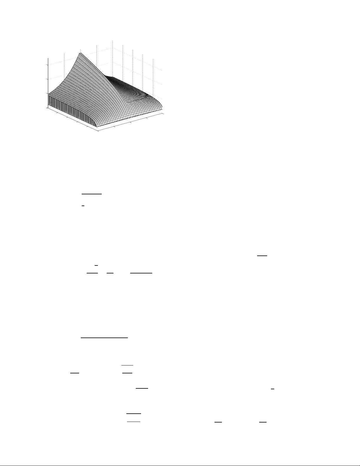
Loss Fluctuations and T emporal Co rrelat ions in Netw ork Qu eues (In vit ed P aper) I. V . Lerner and I . V . Y urkevich School of Physics and As tronom y University of Birmingh am, Ed gbaston Birmingham , B15 2TT , UK Email: { i.v .lerner ,i.yurkevich } @bham.ac.uk A. S. Stepa nenko and C. C. Constantinou School of Engineerin g University of Birmingham, Edgbaston Birmingham , B15 2TT , UK Email: { a.stepanenko,c. constantino u } @bham.ac.uk Abstract —W e co nsider data losses in a single node of a packet- switched Internet-like network. W e employ tw o distinct mo dels, one wi th discrete and the other with continuou s one-dimensional random walks, representing th e state of a q ueue in a router . Both models hav e a built-in critical beha vior with a sharp transition from exponenti ally small to fini te losses. It turns out that the finite capacity of a buffer and the packet-dropping procedure giv e rise to sp ecific bound ary conditions which lead to strong loss ra te fluctuations at the criti cal point even in the absence of such fluctuations in the data arriva l process. I . I N T R O D U C T I O N Many systems, bo th natural and m an-made are organized as complex network s of interco nnected entities: b rain cells [1], interacting molecules in living cells [2], m ulti-species food webs [ 3], social networks [4] and the Intern et [5] are just a fe w examples. In addition to the classical Er d ¨ os–R ´ enyi model fo r rand om networks [6], n ew overarching mo dels of scale-free [7] or small- world [8] networks turn out to describ e real world examples. The se and other network models hav e received extensive attentio n by p hysicists (see Refs. [9], [10] for revie ws). A particularly in teresting problem for a wide ran ge o f com- plex networks is their resiliency to breakdowns. The possibility of rand om or inten tional br eakdowns of the en tire n etwork has been consider ed in the con text of scale-free networks where nodes were randomly or selecti vely r emoved [11], [12], [13], or in the context of small-world networks where a random reduction in the sites’ connectivity leads to a sharp in crease in the o ptimal distance across network which destroys its small- world natur e [13], [14], [1 5]. In all the se mo dels, the site or bond d isorder a cts as an in put which makes them very gen eral and applicable to a wide v ariety of netw orks. Network breakdowns can result not only fr om a ph ysical loss of connectivity b ut fro m an o perationa l failure of some network no des to forward d ata. In the more sp ecific class of commun ication n etworks, this could hap pen due to excessi ve loading of a single node. This could trigger cascades of failures and thu s isolate large parts of the network [16]. In describing the operational failure in a particu lar network node, o ne n eeds to acco unt fo r distinct features of th e dy namically ‘ran dom’ data traffic wh ich can be a rea son for such a breakdown. In this paper we mo del data losses in a single nod e of a pac ket-switched network like th e Intern et. There are two distinct f eatures w hich must be preserved in this case: the discrete character of data pro pagation and the possibility of data overflow in a single n ode. I n the pac ket-switched network data is divided into packets which are r outed fro m sour ce to destination v ia a set of interco nnected no des (rou ters). At each node p ackets are queued in a memory buf fer befor e being serviced , i.e. forwarded to the next nod e. (There are separate buf fers for in coming and outgoing packets but we neglect this for th e sake o f simplicity). Due to th e finite capacity of memory buffers and the stoc hastic n ature o f data traffic, any buf fer can becom e overflo wn wh ich results in p ackets being discar ded . W e consider a model where noticeable data losses in a s ingle memory buffer start when the average rate of r andom packet arriv als approa ches the service rate. Under this condition the mod el has a b uilt-in sharp tra nsition fro m free flow to lossy behavior with a finite fr action of arriving packets being dropp ed. A sharp onset of network co ngestion is familiar to ev eryone using the Internet and was numerically confirmed in different mod els [17]. Here we stress that such a conge stion can originate from a single node. While data loss is natu ral an d in evitable due to the data overflo w , we show that lo ss r ate statistics turn out to be h ighly nontrivial in the r ealistic case of a finite buf fer, where at the critical point the magn itude of fluctu ations can exceed the av erage value, wh ile they obey the cen tral limit theorem on ly in the ( unrealistically) lon g time limit. Such an im portanc e of fluctuations in some inter mediate regime is a defin itiv e feature of mesoscopic physics, albeit the reasons for this are absolutely different (note that even in the case o f electron s, the orig in of the mesoscopic phen omena can be either quan tum or purely classical, see, e.g ., [ 18]). Althou gh we model data ar riv als as a Markovian process, the loss rate at inter mediate times shows long-r ange power -law correlations in time. When excessive data lo sses start, it is more p robab le that they persist for a while, thus impacting on network op eration. The average loss r ate and/o r transpor t delay s were previ- ously studied , e.g., in th e theo ries of bulk queues [1 9], [20] or a jamming transition in traffic flow [21]. What makes . . . . . . . . . . . . . . . . . . . . . . . . . . . . . . . . . . . . . . . . . . . . . . . . . . . . . . . . . . . . . . . . . . . . . . . . . . . . . . . . . . . . . . . . . . . . . . . . . . . . . . . . . . . . . . . . . . . . . . . . . . . . . . . . . . . . . . . . . . . . . . . . . . . . . . . . . . . . . . . . . . . . . . . . . . . . . . . . . . . . . . . . . . . . . . . . . . . . . . . . . . . . . . . . . . . . . . . . . . . . . . . . . . . . . . . . . . . . . . . . . . . . . . . . . . . . . . . . . . . . . . . . . . . . . . . . . . . . . . . . . . . . . . . . . . . . . . . . . . . . . . . . . . . . . . . . . . . . . . . . . . . . . . . . . . . . . . . . . . . . . . . . . . . . . . . . . . . . . . . . . . . . . . . . . . . . . . . . . . . . . . . . . . . . . . . . . . . . . . . . . . . . . . . . . . . . . . . . . . . . . . . . . . . . .. . . .. . . . . . . . . . . . . . . . . . . . . . . . . . . . . . . . . . . . . . . . . . . . . . . . . . . . . . . . . . . . . . . . . . . . . . . . . . . . . . . . . . . . . . . . . . . . . . . . . . . . . . . . . . . . . . . . . . . . . . . . . . . . . . . . . . . . . . . . . . . . . . . . . . . . . . . . . . . . . . . . . . . . . . . . . . . . . . . . . . . . . . . . . . . . . . . . . . . . . . . . . . . . . . . . . . . . . . . . . . . . . . . . . . . . . . . . . . . . . . . . . . . . . . . . . . . . . . . . . . . . . . . . . . . . . . . . . . . . . . . . . . . . . . . . . . . . . . . . . . . . . . . . . . . . . . . . . . . . . . . . . . . . . . . . . . . . . . . . . . . . . . . . . . . . . . . . . . . . . . . . . . . . . . . . . . . . . . . . . . . . . . . . . . . . . . . . . . . . . . . . . . . . . . . . . . . . . . . . . . . . . . . . . . . . . . . . . . . . . . . . . . . . . . . . . . . . . . . . . . . . . . . . . . . . . . . . . . . . . . . . . . . . . . . . . . . . . . . . . . . . . . . . . . . . . . . . . . . . . . . . . . . . . . . . . . . . . . . . . . . . . . . . . . . . . . . . . . . . . . . . . . . . . . . . . . . . . . . . . . . . . . . . . . . . . . . . . . . . . . . . . . . . . . . . . . . . . . . . . . . . . . . . . . . . . . . . . . . . . . . . . . . . . . . . . . . . . . . . . . . . . . . . . . . . . . . . . . . . . . . . . . . . . . . . . . . . . . . . . . . . . . . . . . . . . . . . . . . . . . . . . . . . . . . . . . . . . . . . . . . . . . . . . . . . . . . . . . . . . . . . . . . . . . . . . . . . . . . . . . . . . . . . . . . . . . . . . . . . . . . . . . . . . . . . . . . . . . . . . . . . . . . . . . . . . . . . . . . . . . . . . . . . . . . . . . . . . . . . . . . . . . . . . . . . . . . . . . . . . . . . . . . . . . . . . . . . . . . . . . . . . . . . . . . . . . . . . . . . . . . . . . . . . . . . . . . . . . . . . . . . . . . . . . . . . . . . . . . . . . . . . . . . . . . . . . . . . . . . . . . . . . . . . . . . . . . . . . . . . . . . . . . . . . . . . . . . . . . . . . . . . . . . . . . . . . . . . . . . . . . . . . . . . . . . . . . . . . . . . . . . . . . . . . . . . . . . . . . . . . . . . . . . . . . . . . . . . . . . . . . . . . . . . . . . . . . . . . . . . . . . . . . . . . . . . . . . . . . . . . . . . . . . . . . . . . . . . . . . . .. . . .. . . . . . . . . . . . . . . . . . . . . . . . . . . . . . . . . . . . . . . . . . . . . . . . . . . . . . . . . . . . . . . . . . . . . . . . . . . . . . . . . . . . . . . . . . . . . . . . . . . . . . . . . . . . . . . . . . . . . . . . . . . . . . . . . . . . . . . . . . . . . . . . . . . . . . . . . . . . . . . . . . . . . . . . . . . . . . . . . . . . . . . . . . . . . . . . . . . . . . . . . . . . . . . . . . . . . . . . . . . . . . . . . . . . . . . . . . . . . . . . . . . . . . . . . . . . . . . . . . . . . . . . . . . . . . . . . . . . . . . . . . . . . . . . . . . . . . . . . . . . . . . . . . . . . . . . . . . . . . . . . . . . . . . . . . . . . . . . . . . . . . . . . . . . . . . . . . . . . . . . . . . . . . . . . . . . . . . . . . . . . . . . . . . . . . . . . . . . . . . . . . . . . . . . . . . . . . . . . . . . . . . . . . . . . . . . . . . . . . . . . . . . . . . . . . . . . . . . . . . . . . . . . . . . . . . . . . . . . . . . . . . . . . . . . . . . . . . . . . . . . . . . . . . . . . . . . . . . . . . . . . . . . . . . . . . . . . . . . . . . . . . . . . . . . . . . . . . . . . . . . . . . . . . . . . . . . . . . . . . . . . . . . . . . . . . . . . . . . . . . . . . . . . . . . . . . . . . . . . . . . . . . . . . . . . . . . . . . . . . . . . . . . . . . . . . . . . . . . . . . . . . . . . . . . . . . . . . . . . . . . . . . . . . . . . . . . . . . . . . . . . . . . . . . . . . . . . . . . . . . . . . . . . . . . . . . . . . . . . . . . . . . . . . . . . . . . . . . . . . . . . . . . . . . . . . . . . . . . . . . . . . . . . . . . . . . . . . . . . . . . . . . . . . . . . . . . . . . . . . . . . . . . . . . . . . . . . . . . . . . . . . . . . . . . . . . . . . . . . . . . . . . . . . . . . . . . . . . . . . . . . . . . . . . . . . . . . . . . . . . . . . . . . . . . . . . . . . . . . . . . . . . . . . . . . . . . . . . . . . . . . . . . . . . . . . . . . . . . . . . . . . . . . . . . . . . . . . . . . . . . . . . . . . . . . . . . . . . . . . . . . . . . . . . . . . . . . . . . . . . . ℓ L 0 n . . . . . . . . . . . . . . . . . . . . . . . . . . . . . . . . . . . . . . . . . . . . . . . . . . . . . . . . . . . . . . . . . . . . . . . . . . . . . . . . . . . . . . . . . . . . . . . . . . . . . . . . . . . . . . . . . . . . . . . . . . . . . . . . . . . . . . . . . . . . . . . . . . . . . . . . . . . . . . . . . . . . . . . . . . . . . . . . . . . . . . . . . . . . . . . . . . . . . . . . . . . . . . . . . . . . . . . . . . . . . . . . . . . . . . . . . . . . . . . . . . . . . . . . . . . . . . . . . . . . . . . . . . . . . . . . . . . . . . . . . . . . . . . . . . . . . . . . . . . . . . . . . . . . . . . . . . . . . . . . . . . . . . . . . . . . . . . . . . . . . . . . . . . . . . . . . . . . . . . . . . . . . . . . . . . . . . . . . . . . . . . . . . . . . . Fig. 1. The model of data losses: incoming pack ets randomly arri v e in discrete time interv als and join the queue of lengt h ℓ limite d by the memory buf fer capacity L . Pack ets in front of the queue are served at the same time interv al s. If the queue sticks to the boundary , newl y arri vi ng pack ets are discarde d. present consider ations qualitati vely different is that we analyze fluctuatio ns of a discr ete quantity , the number of discarded packets. Although fluctu ations in n etwork d ynamics were pr e- viously studied (see, e.g. [22]), this was done in the continuous limit fo r the data traffic, throug h measurements or numerical simulations. I I . T H E D I S C R E T E M O D E L The mode of operation of a m emory b uffer is that packets ar - riv e randomly , form a queue in the buffer and are sub sequently serviced . Each packet in the queue has typically a variable length an d is no rmally serviced in fixed-length service units at discrete time intervals o n a first-in first-out basis. Here we choose the simplest non-trivial mo del of this class: ( i) packets have a fixed leng th of two service units; (ii) a rriv al and service intervals coincide. Th e length of the queue after n serv ice intervals, ℓ n , serves as a dynam ical variable which obeys the discrete-time Langevin equ ation, ℓ n +1 = ℓ n + ξ n , (1) where the telegraph no ise ξ n is defined by ξ n =  1 , 0 ≤ ℓ n ≤ L − 1 0 , ℓ n = L , with probab ility p (2) ξ n =  0 , ℓ n = 0 , − 1 , 1 ≤ ℓ n ≤ L , with probab ility 1 − p The a bove means th at the leng th of the queue, measured in service un its, either in creases by on e when o ne packet a rrives and o ne servic e u nit is served, or de creases b y on e when no packet arrives. The boundar y conditions above correspond to discarding a ne wly ar riv ed packet whe n buffer is f ull ( ℓ n = L ) and to a n id le interval when no p acket arrives at an empty buf fer ( ℓ n = 0 ). In a m ore general, con tinuou s model we will remove these r estrictions, allowing for arbitrary quasi- Markovian nature of the input data tr affic. The characteristic features of our results would no t change. The main quantity which character izes con gestion is the packet loss rate which is defined via the n umber of packets discarded during a time in terval N by L N ( n 0 ) = n 0 + N X n = n 0 +1 δ ℓ n ,L δ ℓ n +1 ,L . (3) This me ans tha t the packet is discarded if by th e moment of its arrival the qu eue was at the maximal capacity L as illustrated in Fig. 1 . Thus the lo ss rate (3) is defined entirely by th e processes at the boun dary of the random walk (R W) so that the continuous limit cannot be e xploited . This makes the loss statistics pro foun dly different from, e.g., the thorou ghly studied statistics of first-passage time. W e will consider the average and the variance of the loss rate, which we obtain d irectly from Eq. (3): hL N i = P st ( L ) N G 1 ( L, L ) , (4)  L N 2  = n 0 + N X n,m = n 0 +1  δ ℓ n ,L δ ℓ n +1 ,L δ ℓ m ,L δ ℓ m +1 ,L  = hL N i + 2 P st ( L ) G 2 1 ( L, L ) X n 1 2 ; 1 L +1 , p = 1 2 ; 1 − 2 p 1 − p q L , p < 1 2 ; (7) where q ≡ p/ (1 − p ) . Thus the loss r ate for p > 1 / 2 is of o rder 1, for p = 1 / 2 a small fraction of the b uffer capacity and for p < 1 / 2 an expon entially v anishing fun ction, as expec ted. The matching between the three asymptotic regimes takes place in a narrow region (of width ∼ 1 /L ) aroun d p = 1 2 . The result f or the variance is far more interesting, as it shows significant fluctu ations in the loss rate. It is convenient to express th e variance in terms of the ‘ compr essibility’ defined by h δ L 2 N i ≡ χ N hL N i , δ L N ( n ) = L N ( n ) − hL N i . (8) The compressibility has been exactly c alculated in [23]. Its behavior of χ is illustrated in Fig. 2 which shows its fast increase at the critical point, p = 1 / 2 . −0.1 −0.05 0 0.05 0.1 200 400 600 800 1000 0 10 20 30 2p−1 N χ Fig. 2. compre ssibility χ (for L = 1000 ) shows a f ast increa se of fluctuations in time at the critical point, p = 1 / 2 . For N ≫ N 0 ≡  (2 p − 1) 2 + ( π /L ) 2  − 1 , i.e. in th e limiting steady-state regime the co mpressibility saturates at χ ∞ =    1 −| 2 p − 1 | | 2 p − 1 | , | 2 p − 1 | L ≫ 1 2 3 L, | 2 p − 1 | L ≪ 1 (9) Although it di verges in the the rmody namic limit, L → ∞ and N /L 2 → ∞ , at the transition poin t p = 1 / 2 , the v ariance (8) in this limit rem ains finite and obeys the central limit theo rem. Howe ver , this limit is re achable at the cr itical po int o nly for unrealistically long times N ≫ N 0 ∝ L 2 . I n the interm ediate, practical regime, 1 ≪ N ≪ N 0 , the compressibility rapidly increases with time: χ N = c N 1 / 2 , c = 2 √ 2 π ∞ Z 0 dx x 2 1 − 1 − e − x 2 x 2 ! , (10) so that th e variance exceeds the average v alue of the loss-rate and, as can be sho wn, its distrib ution is no lo nger normal. It is e ven more interesting that in this regime the fluctuations of the loss rate are no longer Markovian as they exhibit long - time correlations. T o show th is, we co nsider the tem poral correlation function of the loss r ate defined by R 2 ( N , M ) ≡ h δ L N (0) δ L N ( M ) i h δ L 2 N i , M > N . In the most rele vant regime, N 0 ≫ N ≫ 1 and M > N , this has been calculated to gi ve R 2 ( N , M ) = pN χ N " e − M (2 p − 1) 2 / 2 r 2 π M − | 2 p − 1 | erfc  | 2 p − 1 | p M / 2  # . (11) At the critical point this reduces using Eq. ( 10) to R 2 ( N , M ) | p =1 / 2 = c − 1 r N 2 π M . (12) This long-time correlation (in spite of the packet arri val b eing Markovian) is anoth er clear sign o f criticality . I I I . T H E C O N T I N U O U S M O D E L Consider th e outpu t buf fer attached to the switching de vice in th e r outer . The speed of th e in put line of the buffer (effecti vely , it is the capacity of the switching fabric) would normally be much bigger than the speed of the output line of the buffer . Hence, we can consider the packet arrival as an instantaneous process. Packets ar riv als are treated as a renewal process. T he capacity of th e buf fer is L ( measured in bits). The leng ths of arr iving pa ckets are treated as rand om (measured in bits). The ser vice (the capacity of th e ou tput link) is co nsidered to be deterministic. Note th at th e packets are put in fr ames befo re b eing sent to th e outpu t link, the correspo nding rando mness (d ue to the rand omness of packet size) is neglected because it is much smaller of the randomness of the ar riv al process (the overhea ds are much smaller th an the typical size of the packet). W e no rmalise the lengths of packets p , the sp eed of th e outpu t link r out and the queue length ℓ b y the size of the buffer L (the size of the buffer is then set to be 1 ). The pr ocedur e is the following: assume that at the mo ment of arri val of a packet of size p , the state of the queue is ℓ , this is followed by the g ap η (ran dom inter-arri val tim e) till the next arriv al. If ℓ + p ≤ 1 then the pac ket joins the queue and the queue length p rior the next arr iv al is ℓ ′ = ℓ + p − η / η 0 if ℓ ′ > 0 and ℓ ′ = 0 otherwise. If ℓ + p > 1 the n the p acket is discarded and the queu e length prior the next arrival is ℓ ′ = ℓ − η /η 0 if ℓ ′ > 0 and ℓ ′ = 0 othe rwise. Here we intro duced the following time scale η 0 ≡ 1 r out , (13) the time required to empty a fu ll buffer provided there are no new arrivals. Assuming that th e maximum packet size is much less tha n 1 (the buf fer size) and the average inco ming traffic rate r in (also n ormalised to the buf fer size) is c lose to the service rate: | r in η 0 − 1 | ≪ 1 (14) we can treat p , η and ℓ as continu ous v ariables. Our aim is to calculate the statistics of the amou nt of the dropp ed traffic and th e service lo st due to idleness o f the output link during time t ≫ ¯ η ( ¯ η is the average inter-arriv al time) in the regime (14 ). In the regime (14) and fo r observation times t ≫ ¯ η , the system can be described by th e Fokker-Planck equatio n as f ollows (in ter ms of the tra nsitional probability density function w ( ℓ ′ , t ; ℓ ) ) ∂ t w ( ℓ ′ , t ; ℓ ) = − a∂ ℓ ′ w ( ℓ ′ , t ; ℓ ) + 1 2 σ 2 ∂ 2 ℓ ′ w ( ℓ ′ , t ; ℓ ) , (15) where a and σ 2 are av erage momen ts o f the chang e of the queue size per unit time a ≡ 1 ∆ t h ∆ ℓ i , σ 2 ≡ 1 ∆ t h ∆ ℓ 2 i , ∆ t → 0 (16) and the fo llowing boun dary a nd in itial conditions ar e imposed J ( ℓ ′ , t ; ℓ ) | ℓ ′ =0 , 1 = 0 , (17) w ( ℓ ′ , t ; ℓ ) | t =0 = δ ( ℓ ′ − ℓ ) (18) where J ( ℓ ′ , t ; ℓ ) ≡ aw ( ℓ ′ , t ; ℓ ) − 1 2 σ 2 ∂ ℓ ′ w ( ℓ ′ , t ; ℓ ) , (19) is th e prob ability curren t. By ∆ t → 0 in eq . (1 6) we mea n that it is much smaller than th e observation time, but large enoug h so that the underlying stochastic processes can be considered as continuou s: ¯ η ≪ ∆ t ≪ t (20) The solution of (15,17,18) can be e xpressed as follo ws w ( ℓ ′ , t ; ℓ ) =2e v ( ℓ ′ − ℓ ) ∞ X k =1 exp  − (4 π 2 k 2 + v 2 ) τ  4 π 2 k 2 + v 2 × [2 π k cos(2 π k ℓ ′ ) + v sin(2 π k ℓ ′ )] × [2 π k cos(2 π k ℓ ) + v sin(2 π k ℓ )] (21) where v ≡ a σ 2 , τ ≡ σ 2 t 2 (22) Note that the solution (21) c an be expressed in terms of θ - function s. For the Laplace tran sform of w ( ℓ ′ , t ; ℓ ) we have W ( ℓ ′ , ǫ ; ℓ ) ≡ L τ w ( ℓ ′ , t ; ℓ ) = 1 2 e v ( ℓ ′ − ℓ ) κ s inh( κ ) × ( 2 v 2 ǫ cosh[ κ ( ℓ ′ + ℓ − 1)] + 2 κv ǫ sinh[ κ ( ℓ ′ + ℓ − 1)] + cosh[ κ ( | ℓ ′ − ℓ | − 1)] + c osh[ κ ( ℓ ′ + ℓ − 1)] ) (23) where κ ≡ p ǫ + v 2 (24) From (2 3) we h av e for th e prob abilities of re turning to th e bound aries W (0 , ǫ ; 0) = 1 ǫ [ κ c otanh( κ ) − v ] W (1 , ǫ ; 1) = 1 ǫ [ κ c otanh( κ ) + v ] (25) These will be used in the n ext sectio n. I V . S TA T I S T I C S O F L O S S E S In this section we will concen trate on the statistics of th e losses due to the buffer overflowing. The correspo nding fo r- mulae for the statistics of the server idleness can be obtained using transformatio n ℓ → 1 − ℓ, v → − v . First, we estimate the size of fluctuations of the losses o n time scale t ≪ 2 /σ 2 . In or der to do that we consider the dynamics o f the system near the bounda ry ℓ = 1 which is governed by the following tr ansitional probability: w 0 ( ℓ ′ , t ; ℓ ) = 1 √ 2 π σ 2 t exp  − a ( ℓ ′ − ℓ ) σ 2 − a 2 t 2 σ 2  ×  exp  − ( ℓ ′ − ℓ ) 2 2 σ 2 t  + exp  − (2 − ℓ ′ − ℓ ) 2 2 σ 2 t  − a σ 2 exp  2 a (1 − ℓ ′ ) σ 2  erfc  2 − ℓ ′ − ℓ + at √ 2 σ 2 t  (26) which is the solu tion of (15) when th e bound ary ℓ = 0 is sen t to − ∞ . The chan ge in the state of the system during time t can then be represented as fo llows: ∆ ℓ ( t ) ≡ ℓ ′ − ℓ = ∆ ℓ 0 ( t ) + ∆ ℓ loss ( ℓ ′ , t ; ℓ ) (27) where ∆ ℓ 0 ( t ) is the cha nge in the state of the system if there was no b ound ary , its statist ics is determined by h ∆ ℓ 0 ( t ) i = a t , h [∆ ℓ 0 ( t )] 2 i = σ 2 t + o( t ) , (28) and ∆ ℓ loss ( ℓ ′ , t ; ℓ ) is the am ount of traffic lost due to b uffer overflo wing. The momen ts of ( 28) can be defined as follo ws h [∆ ℓ ( t )] n i = Z d ℓ ′ d ℓ ( ℓ ′ − ℓ ) n w 0 ( ℓ ′ , t ; ℓ ) p ( ℓ ) (29) where p ( ℓ ) is the stationary distrib ution. For the first two moments (29) in the limit t → 0 we have h ∆ ℓ ( t ) i = at + σ 2 t 2 p (1) , h [∆ ℓ ( t )] 2 i = σ 2 t (30 ) From (27,28,30) we can conclude that h ∆ ℓ loss ( t ) i = σ 2 t 2 p (1) h [∆ ℓ loss ( t )] 2 i + 2 h ∆ ℓ 0 ( t )∆ ℓ loss ( t ) i = o( t ) (31) The first of th e relations ( 31) m eans that ∆ ℓ loss ( ℓ ′ , t ; ℓ ) is no n- zero only if ℓ ′ , ℓ ∼ 1 in the limit t → 0 . T he second relatio n means either h [∆ ℓ loss ( t )] 2 i , h ∆ ℓ 0 ( t )∆ ℓ loss ( t ) i = o( t ) (32) or ∆ ℓ loss ( t ) = − 2∆ ℓ 0 ( t ) + o( √ t ) (33) The relation (33) does no t make sense physically , so in w hat follows we ac cept optio n (32) and show that it is con sistent with the later calculations. Next we lift the r estriction t ≪ 2 /σ 2 . It can be shown that the conditiona l mo ments (with the cond ition that the system was in the state ℓ at the beginn ing of the observation inte rval) can be e xpressed as follows: m ( k ) loss ( t ; ℓ ) = k ! r k loss k Y i =1 t i +1 Z 0 d t i k − 1 Y j =1 w (1 , t j +1 − t j ; 1 ) × w (1 , t 1 ; ℓ ) , t k +1 ≡ t (34) where w ( ℓ ′ , t ; ℓ ) is determined by (21) and r loss ≡ lim t → 0 1 t Z d ℓ ′ Z d ℓ ∆ ℓ loss ( ℓ ′ , t ; ℓ ) = lim t → 0 1 t 1 Z −∞ d ℓ ′ d ℓ ( ℓ ′ − ℓ − at ) w 0 ( ℓ ′ , t ; ℓ ) = σ 2 2 (35) For unconditional moments in the stationary regime we ha ve m ( k ) loss ( t ) ≡ 1 Z 0 d ℓ m ( k ) loss ( t ; ℓ ) p ( ℓ ) = k ! k Y i =1 τ i +1 Z 0 d τ i k − 1 Y j =1 w (1 , t j +1 − t j ; 1 ) · p (1) (36) where τ is define d in (22) and p ( ℓ ) is the stationary solution of (15): p ( ℓ ) = 2 v e 2 vℓ e 2 v − 1 (37) T o calculate m ( k ) loss ( t ) we consider its Laplace transform: M ( k ) loss ( ǫ ) ≡ L τ m ( k ) loss ( t ) = ∞ Z 0 d τ e − ǫτ m ( k ) loss ( t ) = k ! p (1) [ W (1 , ǫ ; 1)] k − 1 1 ǫ 2 (38) where W (1 , ǫ ; 1) is is defin ed by ( 23). From (38) we obtain m (1) loss ( t ) = p (1) τ = p (1) σ 2 t 2 (39) For t he moments (38 ) with k > 1 we can identify the follo wing regimes: M ( k ) loss ( ǫ ) = ( k ! p (1) ǫ − ( k +3) / 2 ǫ ≫ 1 k ! p k (1) ǫ − ( k +1) ǫ ≪ 1 (40) Correspon dingly , for th e moments in t -repr esentation we have m ( k ) loss ( t ) =    k ! p (1) τ ( k +1) / 2 Γ[( k + 3 ) / 2] τ ≪ 1 p k (1) τ k τ ≫ 1 (41) Now we turn our attention to the calculation of the PDF p loss ( x ; t ) of the amount of the lost traffic, x , during time t . T o calculate it we consider its cha racteristic function in the ǫ -repre sentation: ˜ P loss ( s ; ǫ ) ≡ L x P loss ( x ; ǫ ) , P loss ( x ; ǫ ) ≡ L τ p loss ( x ; t ) (42) From (42) we obtain ˜ P loss ( s ; ǫ ) = ∞ X k =0 ( − s ) k k ! ∞ Z 0 d x x k L τ p loss ( x ; t ) = P loss ( ǫ ) + ∞ X k =1 ( − s ) k k ! M ( k ) loss ( ǫ ) (43) where P loss ( ǫ ) = L τ p loss ( t ) , p loss ( t ) = ∞ Z 0 d x p loss ( x, t ) (44) with 1 − p loss ( t ) being the pro bability for the system no t to drop a single pac ket over the period of time t . Su bstituting (38) into (43) we ha ve ˜ P loss ( s ; ǫ ) = P loss ( ǫ ) + p (1) ǫ 2 ∞ X k =1 ( − s ) k [ W (1 , ǫ ; 1)] k − 1 = P loss ( ǫ ) + p (1) ǫ 2 W (1 , ǫ ; 1)  − 1 + 1 1 + sW (1 , ǫ ; 1)  In order that P loss ( s ; ǫ ) did not have a n abno rmal behaviour (in particular, it did not contain terms like δ ( x ) ), we must assume that P loss ( ǫ ) = p (1) ǫ 2 W (1 , ǫ ; 1) (45) Hence, P loss ( x ; ǫ ) = p (1) ǫ 2 W 2 (1 , ǫ ; 1) exp  − x W (1 , ǫ ; 1)  (46) Integrating this relation over x , we recover (45), which shows that our assumption is indeed co rrect. In the regimes of short and long times we hav e p loss ( x ; t ) =        p (1)erfc  x √ 4 τ  τ ≪ 1 δ h x − τ p (1) i τ ≫ 1 (47) and p loss ( t ) =      p (1) r 4 τ π τ ≪ 1 1 τ ≫ 1 (48) The conditio nal PDF ( with the condition that the system dropp ed at least one packet during th e time t ) can be defined as follows w loss ( x ; t ) ≡ p loss ( x ; t ) p loss ( t ) =        r π 4 τ erfc  x √ 4 τ  τ ≪ 1 δ h x − τ p (1) i τ ≫ 1 (49) Now let us compare the results o f the co ntinous approach with those of Section II. T o make the compar ison, we calculate the central moments of losses in a similar w ay as the uncon - ditional ones in Eq . (36). Here we will consider the variance of the losses σ 2 loss ( t ) only in the limit τ ≫ 1 : σ 2 loss ( t ) ≈ m (1) loss ( t )  1 | v | cotanh | v | − sinh − 2 | v |  ≈        2 3 m (1) loss ( t ) | v | ≪ 1 1 | v | m (1) loss ( t ) | v | ≫ 1 (50) In this long-time limit the ratio of th e variance to the square of the average v anishes, so that th e d istribution of d ata lo sses obeys the central limit theorem , as also seen from the secon d line of Eq . (49). T his is essentially in agr eement with the result o f the compressibility χ ∞ in [2 3]. Natur ally , the present consideratio ns are mu ch m ore gen eral as we have not imp osed any artificial limitatio ns on the random input traf fic. Finally , we calculate the correlator of the fluctu ations of losses measured during two time intervals of leng th t 1 and t 2 correspo ndingly an d separated by th e time T : corr( t 1 , t 2 , T ) = 1 Z 0 d ℓ ρ ( t 1 , t 2 , T ) − m (1) loss ( t 1 ) m (1) loss ( t 2 ) where ρ ( t 1 , t 2 , T ) = r 2 loss t 1 Z 0 d t ′ 1 t 2 Z 0 d t ′ 2 w (1 , t ′ 1 + t 2 − t ′ 2 + T ; 1) p (1) with r loss defined in (35). In the regime T ≫ t 1 , t 2 and T ≫ 2 /σ 2 it can be shown that corr( t 1 , t 2 , T ) → T →∞ 0 , (51) as we would expect. In fact, the corr elator goes to zero expo- nentially if v 6 = 0 . I n th e o pposite r egime 2 /σ 2 ≫ T ≫ t 1 , t 2 we have corr( t 1 , t 2 , T ) = m (1) loss ( t 1 ) m (1) loss ( t 2 ) 1 p (1) r 2 π σ 2 T (52) which is again in agreem ent with the results of the discrete- time consideratio ns of Section II, showing the universality of the present approach. V . D I S C U S S I O N A N D C O N C L U S I O N As o ne would expect intu iti vely , loss events separated widely in time are un correlated as sho wn b y equa tion (51). By widely separated in time, we mean that the time separation of the two observation in tervals in which losses occur is much longer than the time over which fluctuations of queue leng th become comparable or mu ch bigger than the buf fer size itself, i.e. 2 /σ 2 . Howe ver , in th e case wh en the separation time is m uch smaller than 2 /σ 2 , the correlation s of loss fluctuations are decaying very , very slowly , as can be seen from eq uation ( 52). Such time intervals are li kely to be compar able or even smaller than the roun d trip times for typical TCP conn ections. TCP is the p rotoco l that contro ls the rate at which data is sent across a network, between a particular sou rce and de stination. Th e exact de tails of the congestion co ntrol o peration o f TCP can be found in [24]. Consideration s o f losses in a n etwork, rather than in a single buf fer , would requ ire kn owledge of the distribution an d correlation s of data traffi c throu gh different buf fers comprising the nod es. The two input parameters, a an d σ 2 in Eq. ( 16) for a sing le buf fer, are determin ed by the network topolog y , the rou ting pr otocol, and the external input traf fic distribution to the network. Of cour se, a detailed kn owledge of all these parameters is never available for a realistic network. W e will consider an an alytically tractable albeit a simplified model with a h omog eneous external traffic (all flows from any source to any d estination are consider ed statistically eq uiv alent). Then the above individual sing le-buf fer input par ameters are straightfor wardly co nnected to the number of flows passing throug h the appro priate buffer . This number , in turn, depends on the to pology , the protocol an d th e external load and is equal to the link-between ness of the co rrespon ding buf fer . Fortunately for our considerations the distribution of these quantities are empirically known through measurements on the Internet [25]. This allowed us to analyze fluctuations and temporal c orrelation s of lo sses in a r ealistic model of the Internet [26]. A C K N O W L E D G E M E N T This work was supported by the EPSRC grant GR/T23725 /01. R E F E R E N C E S [1] M. A. Arbib, The Handbook of B rain Theory and Neural Network s , MIT Press, London (2003). [2] H. Jeong, B. T ombor , R. Albert, Z. N. Oltvai , and A.-L. Barab ´ asi, Nature 407 , 651 (2000 ). [3] J. E. Co hen, F . Briand, and C. M. Newman, Community F ood W ebs: data and the ory , Springer V erlag, Berlin (1990) . [4] F . Liljeros, C. R. Edling, L. A. N. Amaral, H. E. Stanle y , and Y . Aberg, Natur e 411 , 907 (2001). [5] R. Pastor -Satorras and A . V espignani, Phys. Rev . Lett. 86 , 3200 (2001). [6] P . Erd ¨ os and A. R ´ enyi, Publ. Math. I. Hung . 5 , 17 (1960). [7] A.-L. Barab ´ asi and R. Albe rt, Scien ce 280 , 98 (1999 ). [8] D. J. W atts and S. H. Strogatz , Natur e 393 , 440 (1998). [9] D. J. W atts, Small worlds: the dyn amics of net works betwe en order and randomne ss , Prince ton UP (1999). [10] R. Albert an d A.-L. Barab ´ asi, Rev . Mod. Phys. 74 , 47 (200 2). [11] R. Albert, H. Jeong, and A.-L. Barab ´ asi, Natur e 406 , 378 (2000). [12] R. Cohen, K. E rez, D. ben-A vraham, and S. Havl in, Phys. Rev . Lett. 85 , 4626 (2000); ibid 86 , 3682 (2001). [13] L. A. Braunste in, S. V . Buldyre v , R. Cohen, S. Havlin, and H. E. Stanl ey , Phys. Rev . Lett. 91 , 168701 (2003). [14] S. N. Dorogo vtsev and J. F . F . Mendes, Eur ophys. Let t. 50 , 1 (2000). [15] D. J. Asht on, T . C. Jarrett, and N. F . Johnson, Phys. Rev . Lett. 94 , 058701 (2005). [16] Y . Moreno, R. Pastor-Sa torras, A. Vzquez, and A. V espignani, Europhy s. Lett. 62 , 292 (2003). [17] T . Ohira and R. Sawata ri, Phys. Rev . E 58 , 193 (1998); S. G ` abor and I. Csabai, Physica A 307 , 516 (2002). [18] I. V . Lerner , Nucl. Phys. A 560 , 274 (1993). [19] J. W . Cohen, Single Server Queue , Nort h-Holland , Amsterdam (1969 ). [20] M. Schwartz, T elecommuni cation Networks, Proto cols, Mode ling and Analysis , Addison-W esley (1987). [21] O. J. O’Loan, M. R. Eva ns, and M. E. Cat es, Phys. Re v . E 58 , 1404 (1998); T . Naga tani, ibid 58 , 4271 (1998 ). [22] M. A. de Menezes and A.-L. Bara b ´ asi, P hys. Rev . Lett. 92 , 028701 (2004); J. Duch and A . Arenas, ibid 96 , 218702 (2006). [23] I.V . Y urke vich, I.V . Lerner , A.S. Stepanenk o and C.C. Consta ntinou, Phys. Rev . E 74 , 046120 (2006). [24] M. Allmanm, V . Paxson and W . Ste vens, Internet RFC 2581, IE TF (1999). [25] X. Dimitropoulos, D. Kri ouko v , and G. Ril ey . Revi siting in ternet aslevel topolo gy discov ery . In “Passi ve and Acti ve Measurement W orkshop” (P AM), Bost on, MA, (2005). [26] A.S. Ste panenk o, C.C. Const antinou, I.V . Y urke vich, and I.V . Lerner , in pre partion . (2008).