A New Family of Random Graphs for Testing Spatial Segregation

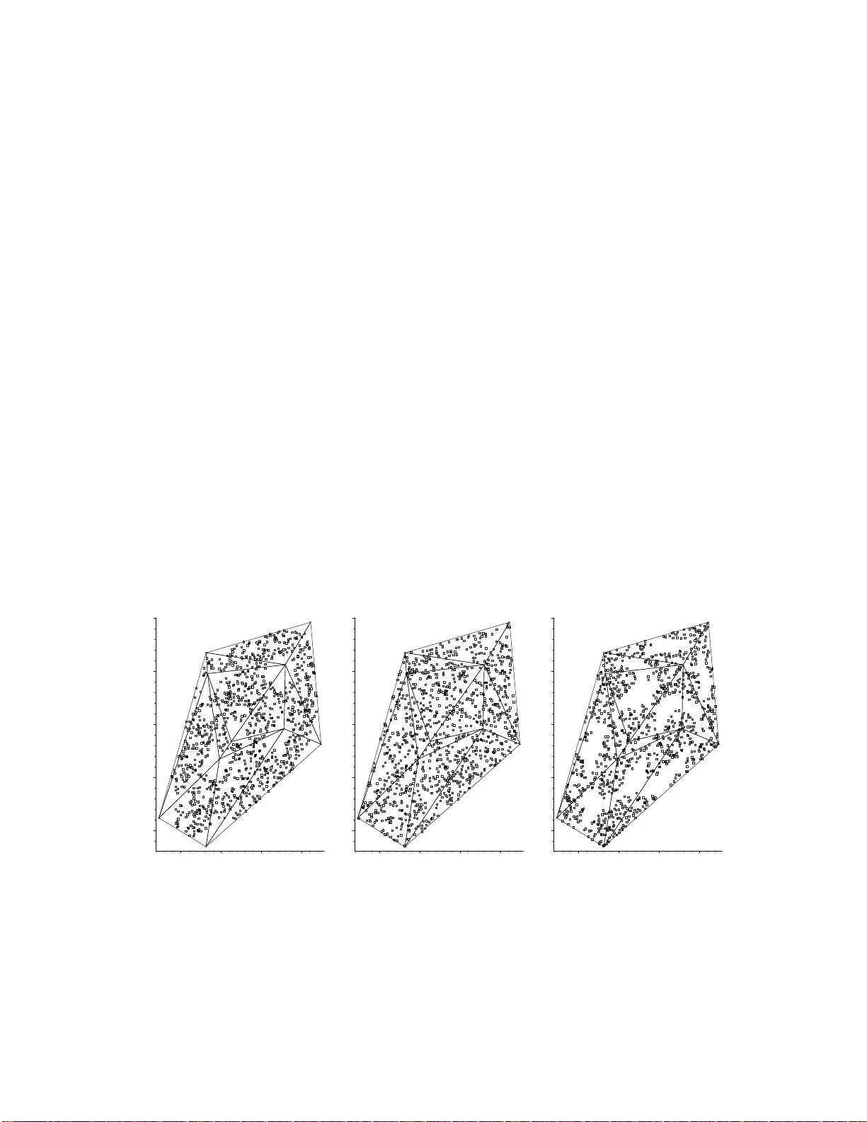
A New F amily of Random Graphs for T esting Spatial Segregation Elv an Ceyhan ∗ , Carey E. Prie b e † , & Da vid J. Marc hette ‡ June 7, 2018 Abstract W e discuss a graph-based approach for testing spatial po in t patterns. This approa c h falls under the category of data-random graphs, whic h hav e been intro duced and used for statistica l pattern reco gnition in recent years. Our g oal is to test complete spatial randomness aga inst segregation and asso ciation betw een t w o or more classes of p oints. T o attain this g oal, w e us e a particular type of parametrized r andom digra ph called proximit y catch digr aph (PCD) whic h is based based on relative p ositions o f the data po in ts from v arious classes. The statistic w e emplo y is the relativ e densit y of the PCD. When scaled prop erly , the relative density o f the P CD is a U -statistic. W e deriv e the asymptotic distribution of the rela tiv e density , using the standard central limit theory o f U -statistics . The finite sample p erformance o f the tes t s tatistic is ev aluated by Monte Carlo simulations, and the asymptotic p erformance is a ssessed via Pitman’s asymptotic efficiency , thereby yielding the optimal parameters for testing. F urthermore, the metho dology discuss ed in this article is a lso v alid for da ta in m ultiple dimensions. Keywor ds: random graph; proximit y catch digra ph; Delaunay triangulation; relative densit y; complete spatia l randomness; segrega tion; a sso ciation ⋆ This w ork was partially suppo rted by Office of Nav al Research Gra n t and Defense Adv a nced Research Pro jects Agency Gra n t. ∗ Corresp onding author. e-mail: elceyhan@ku.e du.tr (E. Ceyhan) ∗ Department of Mathematics, Ko¸ c U nivers it y , Sarıyer, 34450 Istan bul, T urkey (elceyhan@ku .edu.tr) † Department of A pplied Mathematics and Statistics, The Johns Hopkins Univers it y , Baltimore , M D. 21218 (cep@jh u.edu) ‡ Department of A pplied Mathematics and Statistics, The Johns Hopkins Univers it y , Baltimore , M D. 21218 (marc hettedj@nsw c.na vy .mil) 1 1 In tro duction In this artic le, w e discuss a graph-based approac h for testing spatial p oin t patterns. In statistica l literature, the analysis of spatial p oin t patterns in natural p opulations has b een extensiv ely studied and ha v e imp ortan t implications in epidemiology , p opulation biolog y , and ecolo gy . W e in v estiga te th e patte rns of one class with resp ect to other classes, rather than th e pattern of one-cla ss with resp ect to the ground. T he s patial relationships among t w o or m ore group s ha v e imp ortan t imp licat ions esp eciall y for plant sp ecies. See, for exam- ple, Pielou (19 61), Dixon (199 4), and Dixon (2002). Our goal is to test the spatial pattern of complete spati al randomness against spatial segregatio n or association. Complete spatial randomn ess (CSR) is roughly defined as the lac k of spatial inte raction b etw een the p oin ts in a giv en study area. Segreg ation is th e pattern in which p oin ts of one class tend to clus ter together, i.e., form one-class clumps. In asso ciatio n, the p oin ts of one class tend to o ccur more frequent ly aroun d p oin ts from the other cla ss. F or con venience and g eneralit y , w e call t he differen t t yp es of p oin ts as “ classes”, but the class can b e replaced b y an y c haracteristic of an observ atio n at a particular location. F or e xample, the pattern of spatial seg regation has b een inv estigated for species (Diggle (2003)), age classes of p lan ts (Hamill and W right (1986)) and se xes of d ioecious plan ts (Nanami et al. (1999)). W e u se sp ecial graph s called pro ximit y catc h digraphs (PCDs) for testing CSR against segregatio n or asso ciation. In recent y ears, Prieb e et al. (20 01) introd uced a random di- graph related to PCDs (called class co v er catc h digraphs) in R and extended it to m ultiple dimensions. DeVinney et al. (2002), Marchet te and Pr ieb e (2 003), Prieb e et al. (2003b), and Pr ieb e et al. (2003a) demonstr ated relativ ely go od p erformance of it in classification. In t his articl e, w e defi ne a new cla ss of ran dom digraphs (calle d PCDs) and a pply it in testing against segregation or association. A PCD is comprised b y a set of v ertices and a set of (dir ecte d) edges. F or example, in the t wo cla ss case, with classes X and Y , t he X p oin ts are th e v ertices and there is an arc (dir ecte d edge) from x 1 ∈ X to x 2 ∈ X , b ased on a binary relation whic h measures the relativ e all o catio n of x 1 and x 2 with r esp ect to Y p oin ts. By construction, in our PCDs, X p oints further a wa y from Y p oin ts will b e more lik ely to ha ve more arcs directed to other X p oin ts, compared to the X p oints close r to the Y p oin ts. Thus, the relativ e densit y (num b er of a rcs divided b y the total n um b er of p ossible arcs) is a reasonable sta tistic to app ly to this problem. T o illustrate our metho ds, w e p ro vide three artificial d ata sets, one for eac h pattern. These data sets are p lotte d in Figure 1 , where Y p oints are at the ve rtices of the t riangles, and X points are depicte d as squares. Observ e th at we only co nsider the X p oin ts in th e con v ex h u ll of Y p oints; since in the cu rren t form, our pr op osed metho dology only works for such p oint s. Hence we a v oid using a real life example, but use these artificial p attern realizations for illustrativ e purp oses. Under s egrega tion (left) the relativ e densit y of our PCD will b e larger compared to the CSR case ( middle), while under association (righ t) the relativ e dens it y will b e sm aller compared to the CS R case. The statistical tool w e utilize is the asymptotic theory of U -statistics. Prop erly s caled, w e demonstrate that the relativ e densit y of ou r PCDs is a U -statistic , which ha v e asymptotic normalit y by the general cen tral limit theory of U -statistics. The digraph s in trod uced by Prieb e et al. (200 1 ), w hose relativ e d ensit y is also of the U -stat istic form, the asymptotic 2 mean a nd v ariance of the relat iv e densit y is not analytically tracta ble, d ue to ge ometric difficulties encounte red. Ho wev er, the PCD we in tro d uce here is a parametrized family of random digraph s, wh ose relativ e densit y has tractable asymptotic mean and v ariance. Ceyhan and Prieb e in tr od uced an (unparametrized) version of this P CD an d another parametrized family of PCDs in Ceyhan and Prieb e (2003) and C eyhan and Prieb e (2005), resp ectiv ely . Ceyhan and Prieb e (2005) used the domination n um b er (whic h is another statistic b ased on the n um b er of arcs from the v ertices) of the second parametrized family for testing segregation and asso ciation. The domination num b er approac h is appropr iate when b oth classes are comparably large. Ceyhan et al. (2006) used th e relativ e densit y of the same PCD for testing the spatial p atterns. The new parametrized family of PCDs w e introdu ce has more geometric app eal, simpler in distributional parameters in the asymptotic s, and the range of the p arameters is bou nded. Using the Delauna y triangulation of the Y observ atio ns, we will define the p arametrized v ersion of the pro ximit y maps of Ceyh an and Prieb e (2003) in S ectio n 3.1 for wh ic h the calculatio ns —regarding the distribution of the relativ e den sit y— are tractable. W e then can use the r elati v e densit y of the digraph to construct a test o f complete spatial randomness against the alternativ es of segregatio n or asso ciation which are defined explicitly in Sections 2 and 4.1. W e will calculate th e asymptotic distribution of the relativ e densit y for these digraphs, un der b oth the n ull distribution and the alternativ es in S ectio ns 4.2 and 4.3, resp ectiv ely . This pro cedure results in a consisten t test, as will b e sh o w n in Section 5.1. The fin ite sample b eha viour (in terms of p o w er) is analyzed usin g Monte Carlo sim ulatio n in Section 5.2. Th e Pitman asymptotic efficie ncy is analyzed in Section 5.2.3. The m ultiple- triangle case is presente d in S ectio n 5.3 and the extension to higher dimens ions is presented in Section 5.4. All pro ofs are provided in the App endix. 0.2 0.4 0.6 0.8 1 0.2 0.4 0.6 0.8 0.2 0.4 0.6 0.8 1 0.2 0.4 0.6 0.8 0.2 0.4 0.6 0.8 1 0.2 0.4 0.6 0.8 Figure 1: Realizat ions of segregation (left), CSR (middle), and asso ciation (right) for |Y | = 10 and |X | = 1000. Y points are at the v ertices of the triangles, and X p oin ts are squares. 3 2 Spatial P oin t P atterns F or simplicit y , w e describ e the spatial p oint patterns for t w o-cla ss p opulations. T he n ull h yp othesis fo r spatia l patte rns ha v e b een a con tro versial topic in ecology from the early da ys (Gotelli and Gra ves (1996)). But i n general, the null hyp othesis consists of t wo rand om pattern t yp es: complete sp atial randomness or r andom lab eling. Under c ompl ete sp atial r andomness (CSR) for a spatial p oin t pattern { X ( D ) , A ( D ) ∈ R 2 } wher e A ( · ) denotes the area f unctional, w e hav e (i) give n n even ts in d omain D , the ev en ts are an indep end en t rand om s ample f rom a uniform distrib ution on D ; (ii) there is no sp atial interact ion. F urthermore, the n um b er of ev en ts in any planar region with area A ( D ) follo ws a P oisson distribution w ith mean λ · A ( D ), whose pr obabilit y mass function is giv en b y f X ( D ) ( x ) = e − λ · A ( D ) ( λ · A ( D )) x x ! , x ∈ { 0 , 1 , 2 , . . . } where λ is the in tensit y of the P oisson distribution. Under r andom lab eling , class lab els are assigned to a fixed set of points randomly s o that the lab els are ind ep enden t of the locations. Th us, r andom lab eling is less restrictiv e than CS R. Bu t conditional on a set of p oin ts from CS R, b oth pro cesses are equiv alent. W e only consider a s p ecial case of CSR as our n ull hyp othesis in this article. That is, only X p oin ts are assum ed to b e uniformly distributed o v er the conv ex h ull of Y p oints. The alternativ e p atterns fall un der t w o m a jor categories called asso ci ation and se gr e ga- tion . Asso ciation o ccurs if the p oints from th e t w o classes together form clum ps or clusters. That is, asso ciation o ccurs wh en member s of one class hav e a tendency to attract m em b ers of the other class, as in sym biotic sp ecies, so that the X i will tend to cluster around the elemen ts of Y . F or example, in p lan t biology , X p oint s might b e p arasitic plants exploiting Y p oin ts. As another example, X and Y p oin ts migh t r epresen t mutualistic plan t s p ecies, so they dep end on eac h other to survive. In epid emiolog y , Y points migh t b e contaminan t sources, su c h as a nuclea r reactor, or a factory emitting to xic gases, and X p oin ts might b e the r esidence of cases (incidences) of certain diseases caused by the con taminan t, e.g., some t yp e of cancer. Se gr e gation occurs if the mem b ers of the same class tend to b e clump ed or clustered (see, e.g., Pielou (1961)). Man y differen t forms of segregation are p ossible. Ou r metho ds will b e useful only for th e segregation p atterns in whic h the tw o classes more or less share the same supp ort (habita t), and mem b ers of one class ha ve a tendency to r ep el mem b ers of the other class. F or instance, it ma y b e the case that one t yp e of plan t do es not gro w well in the vicinit y of another t yp e of plan t, and vice v ersa. This implies, in our notation, that X i are unlik ely to b e located n ear an y elemen ts of Y . See, for instance, (Co omes et al. (1999); Dixon (1994)). In plan t bio logy , Y p oin ts might r epresen t a tree sp ecies with a large canop y , so that, other plants ( X p oin ts) that need ligh t cannot gro w around these trees. As a nother in teresting but con trived example, consider the arsonist who w ishes to sta rt fires with maxim um du ration time (hence maxim um damage), so th at he starts the fires at the furthest p oin ts p ossib le from fire houses in a cit y . Th en Y p oin ts could b e the fire houses, wh ile X p oin ts will b e the lo cations of arson ca ses. 4 W e consider c ompletely mapp e d data , i.e., the locations of all ev ents in a defined space are observed rather than sparsely s ampled data (only a rand om subset of lo cations are observ ed). 3 Data-Random Pro ximit y Catc h Digraphs In general, in a ran dom digraph , there is an arc b et w een tw o vertice s, w ith a fixed proba- bilit y , indep end en t of other arcs and vertex pairs. Ho w ever, in our approac h, arcs with a shared vertex w ill b e dep en den t. Hence the n ame data-r andom digr aphs . Let (Ω , M ) be a measur able space and consider a fun ction N : Ω × 2 Ω → 2 Ω , where 2 Ω represent s the p ow er set of Ω. Then giv en Y ⊆ Ω, the pr oximity map N Y ( · ) = N ( · , Y ) : Ω → 2 Ω asso ciate s a pr oximity r e gion N Y ( x ) ⊆ Ω w ith eac h p oint x ∈ Ω. The region N Y ( x ) is defined in terms of the distance b et w een x and Y . If X n := { X 1 , X 2 , · · · , X n } is a s et of Ω-v alued random v ariables, then the N Y ( X i ) , i = 1 , · · · , n , are random sets. I f the X i are indep endent and iden ticall y d istributed, then so are the r andom sets, N Y ( X i ). Define the data-random pro ximit y catc h d igraph D with v ertex set V = { X 1 , · · · , X n } and arc s et A b y ( X i , X j ) ∈ A ⇐ ⇒ X j ∈ N Y ( X i ) wh ere p oin t X i “catc hes” p oin t X j . The random digraph D dep ends on the (joi n t) d istribution of the X i and on th e map N Y . The adjectiv e pr oximity — f or the catc h digraph D and for the map N Y — comes f rom thinking of the region N Y ( x ) as represen ting those p oin ts in Ω “close” to x (T oussaint (1980) and Jaromczyk and T oussain t (1992)). The r elative density of a d igraph D = ( V , A ) of order |V | = n (i.e., n um b er of vertice s is n ), denoted ρ ( D ), is defined as ρ ( D ) = |A| n ( n − 1) where | · | denotes the set cardinalit y fu nctional (Janson et al. (2000)). Th us ρ ( D ) represent s the ratio of the n um b er of arcs in the digraph D to the n um b er of arcs in the complete sym metric d igraph of order n , n amely n ( n − 1). If X 1 , · · · , X n iid ∼ F , then the relativ e densit y of the asso ciated data-random pro x imit y catc h digraph D , denoted ρ ( X n ; h, N Y ), is a U-statistic, ρ ( X n ; h, N Y ) = 1 n ( n − 1) X X i 0. The asymptotic v ariance of ρ n , Co v [ h 12 , h 13 ], dep ends on only F and N Y . Thus, we need determine only E [ h 12 ] and Co v [ h 12 , h 13 ] in order to obtain the n ormal approxima tion ρ n appro x ∼ N ( E [ ρ n ] , V ar [ ρ n ]) = N  E [ h 12 ] 2 , Co v [ h 12 , h 13 ] n  for large n. (6) 3.1 The τ -F actor Cen tral Sim ilarit y Proxim it y Catc h Digraphs W e define the τ -factor cen tr al similarit y proximit y map briefly . Let Ω = R 2 and let Y = { y 1 , y 2 , y 3 } ⊂ R 2 b e three n on-collinea r p oints. Denote the triangle — in cluding the interior — formed b y the p oint s in Y as T ( Y ). F or τ ∈ [0 , 1], define N τ Y to b e th e τ - factor c entr al similarity pr oximity ma p as follo ws; see also Figure 2. Let e j b e the edge op p osite v ertex y j for j = 1 , 2 , 3, and let “edge regions” R ( e 1 ), R ( e 2 ), R ( e 3 ) p artitio n T ( Y ) u sing segments from the cen ter of mass of T ( Y ) to th e vertice s. F or x ∈ T ( Y ) \ Y , let e ( x ) b e the edge in w hose region x falls; x ∈ R ( e ( x )). If x falls on the b oun dary of t w o edge regions w e assign e ( x ) arbitrarily . F or τ ∈ (0 , 1], the τ -factor cen tral simila rit y proximit y region N τ C S ( x ) = N τ Y ( x ) is defined to b e the tr iangle T τ ( x ) with the f ollo wing prop erties: (i) T τ ( x ) has an edge e τ ( x ) parallel to e ( x ) su c h that d ( x, e τ ( x )) = τ d ( x, e ( x )) and d ( e τ ( x ) , e ( x )) ≤ d ( x, e ( x )) where d ( x, e ( x )) is the Euclidean (p erp endicular) d istance from x to e ( x ), (ii) T τ ( x ) has th e same orien tation as and is similar to T ( Y ), (iii) x is at the cen ter of mass of T τ ( x ). Note that (i) implies the “ τ -factor”, (ii) imp lies “similarit y”, and (iii) imp lies “ce n tral” in the name, τ -factor c entr al similarity pr oximity map . Notic e that τ > 0 implies that x ∈ N τ C S ( x ) and τ ≤ 1 imp lies that N τ C S ( x ) ⊆ T ( Y ) for all x ∈ T ( Y ). F or x ∈ ∂ ( T ( Y )) and τ ∈ [0 , 1], we defin e N τ C S ( x ) = { x } ; for τ = 0 and x ∈ T ( Y ) w e al so define N τ C S ( x ) = { x } . Let T ( Y ) o b e the interior of the triangle T ( Y ). Then for all x ∈ T ( Y ) o the edges e τ ( x ) and e ( x ) are co inciden t iff τ = 1. O bserv e that the central similarit y pro ximit y map in 6 y 3 y 1 e 3 = e ( x ) d ( x, e ( x )) d ( x, e τ ( x )) = τ d ( x, e ( x )) x e τ =1 / 2 ( x ) y 2 M C Figure 2: Construction of τ -factor cen tral similarit y pro ximit y region, N 1 / 2 C S ( x ) (sh aded region). (Ceyhan and Priebe (2003)) is N τ C S ( · ) with τ = 1. Hence by d efinition, ( x, y ) is an arc of the τ -factor ce n tral similarity PCD iff y ∈ N τ C S ( x ). Notice that X i iid ∼ F , with the additional assump tion that the non-degenerate t w o- dimensional p robabilit y densit y function f exists with supp ort in T ( Y ), implies that the sp ecial case in the construction of N τ C S — X falls on the bou ndary of tw o edge regio ns — o ccurs with p robabilit y zero. F or a fixed τ ∈ (0 , 1], N τ C S ( x ) get s larger (in area) as x gets further a wa y from the edges (or equiv alen tly gets closer to the cen ter of mass, C M ) in the sense that as d ( x, e ( x )) increases (or equiv alently d ( C M , e τ ( x )) decrease s. Hence for p oin ts in T ( Y ), the fu rther the p oin ts a w a y f rom the v ertices Y (or closer the p oin ts to C M in the ab ov e sense), the larger the area of N τ C S ( x ). Hence, it is more likel y f or suc h p oin ts to catc h other p oint s, i.e., ha v e more arcs directed to other points. T herefore, if more X p oin ts are clustered around the cente r of mass, then the digraph is more lik ely to h a ve more arcs, hence larger relativ e densit y . So, und er seg regation, relativ e densit y is exp ected to b e larger than that in CSR or asso ciatio n. On the other hand, in the case of asso ciation, i.e., when X p oin ts are clustered around Y p oin ts, the regions N τ C S ( x ) tend to b e smaller in area, hence, catc h less p oin ts, thereb y r esulting in a small num b er of arcs, or a smaller relativ e densit y compared to C SR or segregation. See, for example, Figure 3 with 3 Y p oints, and 20 X p oin ts for segregation (top left), CSR (middle left) and asso ciation (b ottom r igh t). The co rresp ondin g arcs in the τ -factor cen tral similarit y PCD with τ = 1 are plotte d in the righ t in Figure 3. The corresp onding relativ e densit y v alues (for τ = 1) are .1395, .2579, and .0974, resp ectiv ely . F urthermore, for a fixed x ∈ T ( Y ) o , N τ C S ( x ) gets larger ( in area) a s τ increases. So, as τ increases, it is more likel y to ha ve more arcs, hence larger relativ e densit y for a give n realizatio n of X p oints in T ( Y ). 7 Figure 3: Realizat ions of segregation (left), CSR (middle), and asso ciation (right) for |Y | = 3 and |X | = 20. Y p oin ts are at the v ertices of the triangle, an d X p oin ts are squares. The n u m b er of arcs with τ = 1 are 98, 53 , and 37, resp ectiv ely . S o, relativ e densit y v alues are .258, .139, and .097, resp ectiv ely . 8 4 Asymptotic Distribution of the Relativ e Densit y W e first describ e the null and alternativ e p atte rns we consider briefly , and th en pr o vid e the asymptotic d istribution of the relativ e dens it y for these patterns. There are t w o ma j or t yp es of asymptotic structur es for spatial d ata (Lahiri (1996)). In the first, any t wo observ ations are required to b e at least a fixed distance apart, h ence as the num b er of observ ations increase, the region on wh ic h th e pro cess is observed ev en tually b ecomes un b ounded. This t yp e of sampling structure is call ed “increasing domain asymp- totics”. In the second typ e, the r egion of interest is a fixed b ounded regio n and more and more p oint s are observed in this r egion. Hence th e min im um distance b et ween data p oin ts tends to ze ro a s the sample size tends to infi nit y . T his t yp e of structure is ca lled “ infill asymptotics”, due to Cr essie (1991 ). The s ampling structur e for ou r asymptotic analysis is infill, as only the size of the t yp e X pro cess tend s to infi nit y , while the sup p ort, the conv ex h ull of a giv en set of p oints from t yp e Y pro cess, C H ( Y ) is a fixed b ound ed region. 4.1 Null and Alternativ e P atterns F or statistical testing for segregatio n and asso ciation, the null hyp othesis is generally some form of c omp lete sp atial r and omness ; th us w e consider H o : X i iid ∼ U ( T ( Y )) . If it is desired to h a ve th e sample size b e a random v ariable, w e ma y co nsider a spatial P oisson p oint pro cess on T ( Y ) as our n u ll h yp othesis. Geometry Inv ariance Prop erty W e first present a “geometry inv ariance” r esult that will simplify our calc ulations by allo wing us to co nsider the sp ecial case of th e equilateral triangle. Theorem 1: Let Y = { y 1 , y 2 , y 3 } ⊂ R 2 b e th ree non -coll inear p oin ts. F or i = 1 , · · · , n let X i iid ∼ F = U ( T ( Y )), the u niform distr ibution on the triangle T ( Y ). Then for any τ ∈ [0 , 1] the distribution o f ρ n ( τ ) := ρ ( X n ; h, N τ C S ) is in dep endent of Y , hence the geo metry of T ( Y ). Based on Theorem 1 and our uniform n ull hyp othesis, we ma y assume that T ( Y ) is the stand ard equilateral triangle with Y =  (0 , 0) , (1 , 0) ,  1 / 2 , √ 3 / 2  , h enceforth. F or our τ -factor cen tral similarit y proximit y map and uniform n ull hypothesis, the asymptotic null distribution of ρ n ( τ ) = ρ ( X n ; h, N τ C S ) as a fun ction of τ can b e deriv ed. Let µ ( τ ) := E [ ρ n ], then µ ( τ ) = E [ h 12 ] / 2 = P ( X 2 ∈ N τ C S ( X 1 )) is the p robabilit y of an arc o ccurring b et w een an y t w o v ertices and let ν ( τ ) := Co v [ h 12 , h 13 ]. W e define t w o simple classes of alternativ es, H S ε and H A ε with ε ∈  0 , √ 3 / 3  , for seg- regation and asso ciation, r esp ectiv ely . See also Figure 4. F or y ∈ Y , let e ( y ) denote the edge of T ( Y ) opp osite v ertex y , and for x ∈ T ( Y ) let ℓ y ( x ) denote the lin e paralle l to e ( y ) through x . Th en d efine T ( y , ε ) =  x ∈ T ( Y ) : d ( y , ℓ y ( x )) ≤ ε  . Let H S ε b e the mo d el u nder whic h X i iid ∼ U  T ( Y ) \ ∪ y ∈Y T ( y , ε )  and H A ε b e the mo del under wh ic h X i iid ∼ U  ∪ y ∈Y T  y , √ 3 / 3 − ε   . The s haded region in Figure 4 is the supp ort for segregat ion 9 y 2 = (1 , 0) y 1 = (0 , 0) y 3 = (1 / 2 , √ 3 / 2) M C ε ε ε Figure 4: An example for the seg regation alternativ e for a partic ular ε (shad ed r egion), and its complement is for th e asso ciation alternativ e (un shaded r egion) on the sta ndard equilateral triangle. for a particular ε v alue; and its complemen t is the su pp ort for the association alternativ e with √ 3 / 3 − ε . Thus the segregat ion model excludes the p ossib ilit y of any X i o ccurring near a y j , and the association m od el requires that all X i o ccur near a y j . The √ 3 / 3 − ε in the definition of the asso ciation alternativ e is so that ε = 0 yields H o under b oth classes of alternativ es. W e consider these t yp es of al ternativ es among many other p ossibilities, since relativ e density is geomet ry in v arian t for these alternativ es as the alternativ es are defined with parallel lines to the edges. Remark: These definitions of the alt ernativ es a re g iv en for the standard e quilateral triangle. Th e geometry in v ariance result of T heorem 1 from Section 4.1 still holds under the alternativ es, in the follo win g sense. If, in an arbitrary triangle, a small p ercent age δ · 100% where δ ∈ (0 , 4 / 9) of th e area is carv ed a w ay as forbidd en from eac h v ertex using line segmen ts parallel to the opp osite edge , then un der the transformation to the standard equilateral triangle this will result in the alternativ e H S √ 3 δ/ 4 . This argumen t is for segregation with δ < 1 / 4; a similar constru ction is av ailable for the other cases. 4.2 Asymptotic Normalit y Unde r t he Null Hyp othesis By detailed geometric probabilit y calculatio ns pro vided in the App endix, the mean and the asymptotic v ariance of the relati v e d ensit y of the τ -factor pr o ximity catc h digraph ca n b e calculated explicitly . T he cen tral limit theorem f or U -statistics then establishes th e asymptotic normalit y under the un iform null hyp othesis. These r esults are summarized in the follo wing theorem. 10 Theorem 2: F or τ ∈ (0 , 1], the rela tiv e densit y of th e τ -factor cen tral similarity p ro x- imit y digraph conv erges in la w to the n ormal distribution, i.e., as n → ∞ , √ n ( ρ n ( τ ) − µ ( τ )) p ν ( τ ) L − → N (0 , 1) (7) where µ ( τ ) = τ 2 / 6 (8) and ν ( τ ) = τ 4 (6 τ 5 − 3 τ 4 − 25 τ 3 + τ 2 + 49 τ + 14) 45 ( τ + 1)(2 τ + 1)( τ + 2) (9) F or τ = 0, ρ n ( τ ) is degenerate for all n > 1. See the Ap p endix for the deriv ation. Consider the form of the mean and the v ariance fu nctions, whic h are depicted in Figure 5. Note that µ ( τ ) is monotonica lly increasing in τ , since N τ C S ( x ) increases with τ for all x ∈ T ( Y ) o . Note also th at µ ( τ ) is co n tin uous in τ with µ ( τ = 1) = 1 / 6 and µ ( τ = 0) = 0. Regarding the asymptotic v ariance, n ote that ν ( τ ) is contin uou s in τ and ν ( τ = 1) = 7 / 135 and ν ( τ = 0) = 0 —there are no a rcs when τ = 0 a.s.— whic h explains wh y ρ n ( τ = 0) is degenerate. 0 0.02 0.04 0.06 0.08 0.1 0.12 0.14 0.16 0.2 0.4 0.6 0.8 1 P S f r a g r e p l a c e m e n t s τ µ ( τ ) 0 0.01 0.02 0.03 0.04 0.05 0.2 0.4 0.6 0.8 1 P S f r a g r e p l a c e m e n t s τ µ ( τ ) ν ( τ ) Figure 5: Result of Th eorem 2: asymp totic n ull mean µ ( τ ) = µ ( τ ) (left) and v ariance ν ( τ ) = ν ( τ ) (right), from Equ ations (8) and (9), resp ectiv ely . As an exa mple of the limiting distribu tion, τ = 1 / 2 yields √ n  ρ n (1 / 2) − µ (1 / 2 )  p ν (1 / 2) = r 2880 n 19  ρ n (1 / 2) − 1 / 2 4  L − → N (0 , 1) or equiv alent ly , ρ n (1 / 2) approx ∼ N  1 24 , 19 2880 n  . 11 The finite sample v ariance and s k ewn ess may b e d eriv ed analytically in muc h the same w a y as w as Co v [ h 12 , h 13 ] for the asymptotic v ariance. In fact , the e xact distr ibution of ρ n ( τ ) is, in principle, a v ailable b y successiv ely conditioning on the v alues of the X i . Alas, while the joint d istribution of h 12 , h 13 is a v ailable, the join t d istribution of { h ij } 1 ≤ i 0. ρ n ( τ ) is degenerate when ν S ( τ , ε ) = 0. L ik ewise, under H A ε , √ n  ρ n ( τ ) − µ A ( τ , ε )  L − → N  0 , ν A ( τ , ε )  for the v alues of the p air ( τ , ε ) for whic h ν A ( τ , ε ) > 0. ρ n ( τ ) is d egenerate when ν A ( τ , ε ) = 0. Notice that under the asso ciat ion alternativ es any τ ∈ (0 , 1] yields asymptotic normalit y for all ε ∈  0 , √ 3 / 3  , while und er the segrega tion alternativ es only τ = 1 yields this universal asymptotic n ormalit y . 5 The T est and A nalysis The relativ e d ensit y of the cen tral similarit y proximit y catc h digraph is a test statistic for the segregation/association alternativ e; rejecting for extreme v alues of ρ n ( τ ) is appr opriate since under segregation, w e exp ect ρ n ( τ ) to b e large; while under asso ciation, w e exp ect ρ n ( τ ) to b e small. Using the test stat istic R ( τ ) = √ n  ρ n ( τ ) − µ ( τ )  p ν ( τ ) , (10) whic h is the norm alize d relativ e density , the asymptotic critical v alue for the one-sided lev el α test ag ainst seg regation is giv en b y z α = Φ − 1 (1 − α ) . Against segregation, the test rejects for R ( τ ) > z α and against association, the test rejects for R ( τ ) < z 1 − α . F or the example patterns in Figure 3, R ( τ = 1) = 1 . 792 , − . 534, and -1.361 , resp ectiv ely . 5.1 Consistency of the T ests Under the Alternativ es Theorem 4: Th e test against H S ε whic h rejects for R ( τ ) > z α and the test aga inst H A ε whic h rejects for R ( τ ) < z 1 − α are consistent for τ ∈ (0 , 1] and ε ∈  0 , √ 3 / 3  . In f act, the analysis of the means u nder the alternativ es rev eals more than what is required fo r co nsistency . Under segregation, the a nalysis indicates that µ S ( τ , ε 1 ) < µ S ( τ , ε 2 ) for ε 1 < ε 2 . O n the other hand, u nder asso ciation, the analysis in dicates that µ A ( τ , ε 1 ) > µ A ( τ , ε 2 ) for ε 1 < ε 2 . 13 5.2 Mon te Carlo P o wer Analysis In t his secti on, we asses the fi nite samp le b ehaviour of the relativ e densit y usin g Mon te Carlo sim ulations for testing CS R against segregation or asso ciatio n. W e p ro vide the k ernel densit y estimate s, empirical significance lev els, and empirical p o w er estimates un der the n ull case an d v arious segregation and association alt ernativ es. 5.2.1 M on te Carlo P o wer Analysis for Segregation Alternativ es In Figures 8 and 9, w e present the ke rnel densit y estimate s under H o and H S ε with ε = √ 3 / 8 , √ 3 / 4 , 2 √ 3 / 7. Observe that with n = 10 , and ε = √ 3 / 8, the density estimates are v ery similar implying small p o wer; and as ε gets larger, the separation b et ween the null and alternativ e curves gets larger, hence the p o w er gets larger. With n = 10, 10000 Mon te C arlo replicates yield p o w er estimates b β S mc ( ε ) = . 0994 , . 9777 , 1 . 000 , resp ectiv ely . With n = 100, there is more separation b et ween the n ull and alt ernativ e curv es at eac h ε , which implies that p o wer incr eases as ε increases. With n = 100, 1000 Mon te Carlo replicates yield b β S mc ( ε ) = . 5444 , 1 . 000 , 1 . 000. 0.00 0.05 0.10 0.15 0.20 0.25 0 5 10 15 P S f r a g r e p l a c e m e n t s kernel density estimate relative density 0.0 0.1 0.2 0.3 0.4 0.5 0.6 0 5 10 15 P S f r a g r e p l a c e m e n t s kernel density estimate relative density 0.0 0.2 0.4 0.6 0.8 1.0 0 5 10 15 P S f r a g r e p l a c e m e n t s kernel density estimate relative density Figure 8: Kernel densit y estimates for the null (solid) and the seg regation alt ernativ e H S ε (dashed) with τ = 1 / 2, n = 10, N = 10000, and ε = √ 3 / 8 (left), ε = √ 3 / 4 (middle), and ε = 2 √ 3 / 7 (right) . 0.02 0.04 0.06 0.08 0.10 0.12 0 10 20 30 40 50 P S f r a g r e p l a c e m e n t s kernel density estimate relative density 0.0 0.1 0.2 0.3 0.4 0 10 20 30 40 50 P S f r a g r e p l a c e m e n t s kernel density estimate relative density Figure 9: Kernel densit y estimates fo r th e null (solid) and the segrega tion alternativ e H S √ 3 / 4 (dashed) for τ = 1 / 2 with n = 10 and N = 10000 (left) an d n = 100 and N = 1000 (right). 14 F or a giv en alternativ e and sample size, w e may consider analyzing the p ow er of th e test — u sing the asymptotic critical v alue (i.e., th e normal approximati on)— as a fu nction of τ . Figure 10 presents a Mo n te Carlo in v estiga tion of p ow er against H S √ 3 / 8 , H S √ 3 / 4 as a function of τ f or n = 10. The corresp onding empirical significance leve ls and p o w er estimates are present ed in T able 2 . The empirical significance lev els, b α n =10 , are all greater than . 05 with smallest b eing . 086 8 at τ = 1 . 0 whic h h a ve the empirical p o w er b β 10 ( √ 3 / 8) = . 2289, b β 10 ( √ 3 / 4) = . 9969. Ho we v er, th e empirical sig nificance lev els imply that n = 10 is not large enough for norm al appro ximation. Notice that as n gets larger, the empirical significance lev els g ets closer to . 05 (except for τ = 0 . 1), bu t still are all grea ter than . 05 , which in dicates that for n ≤ 100, the test is lib eral in rejecting H o against segrega tion. F urthermore, as n increases, for fixed ε the empirical p o wer estimates increase, the empir ical significance lev els get closer to . 05; and f or fixed n as τ in creases p o w er estimates get larger. Therefore, for segregation, w e recommend the use of large τ v alues ( τ . 1 . 0). 0.2 0.4 0.6 0.8 1.0 0.0 0.2 0.4 0.6 0.8 1.0 τ P S f r a g r e p l a c e m e n t s power 0.2 0.4 0.6 0.8 1.0 0.0 0.2 0.4 0.6 0.8 1.0 τ P S f r a g r e p l a c e m e n t s power Figure 10: Mon te Carlo p o w er using the asymptotic critical v alue against s egrega tion alternativ es H S √ 3 / 8 (left), H S √ 3 / 4 (righ t), as a function of τ , for n = 1 0 an d N = 1000 0. The circles represent the empirical significance lev els wh ile triangles r epresen t the empirical p o w er v alues. 5.2.2 M on te Carlo P o wer Analysis for Asso ciation Alternatives In Figures 11 and 12, we present the kernel densit y estimates under H o and H A ε with ε = √ 3 / 21 , √ 3 / 12 , 5 √ 3 / 24. Observ e that with n = 10, the densit y estimates are v ery similar for all ε v alues (with sligh tly more separation for larger ε ) implying small p o w er. 10000 Monte Carlo replicates yield p o w er estimates b β A mc ≈ 0. With n = 100, there is more separation b et w ee n th e null and alternativ e curve s at eac h ε , whic h implies that p o w er increases as ε increases. 1000 Monte Carlo replicates yield b β A mc = . 324 , . 634 , . 634, resp ectiv ely . F or a giv en alternativ e and sample size, w e may consider analyzing the p ow er of th e test — using th e asymptotic critical v alue— as a function of τ . The empirical significance lev els and p o wer estimat es against H A ε , with ε = √ 3 / 12 , 5 √ 3 / 24 as a fun ctio n of τ for n = 10 are presented in T able 2. The empir ical significance lev el closest 15 τ .1 .2 .3 .4 .5 . 6 .7 .8 .9 1.0 n = 10, N = 10000 b α S ( n ) .0932 .1916 .1740 .1533 .1101 .0979 .1035 .0945 .0883 .0868 b β S n ( τ , √ 3 / 8) .1286 .2630 .2917 .2811 .2305 .2342 .2526 .2405 .233 4 .2289 b β S n ( τ , √ 3 / 4) .5821 .9011 .9824 .9945 .9967 .9979 .9990 .9985 .998 3 .9969 n = 20, N = 10000 b α S ( n ) .2018 .1707 .1151 .1099 .0898 .0864 .0866 .0800 .0786 .0763 b β S n ( τ , √ 3 / 8) .2931 .3245 .2744 .3021 .2844 .2926 .3117 .3113 .311 9 .3038 n = 100, N = 1000 b α S ( n ) .155 .101 .080 .077 .075 .066 .065 .063 .066 .069 b β S n ( τ , √ 3 / 8) .574 .574 .612 .655 .709 .742 .774 .786 .793 .793 T able 1 : The empirical significance lev el and empirical pow er v alues u nder H S ε for ε = √ 3 / 8 , √ 3 / 4 at α = . 05. 0.0 0.1 0.2 0.3 0.4 0 5 10 15 20 P S f r a g r e p l a c e m e n t s kernel density estimate relative density 0.0 0.1 0.2 0.3 0.4 0 5 10 15 P S f r a g r e p l a c e m e n t s kernel density estimate relative density 0.00 0.05 0.10 0.15 0 5 10 15 20 P S f r a g r e p l a c e m e n t s kernel density estimate relative density Figure 11: Kernel d ensit y estimates for the null (solid) and the asso ciatio n alternative H A ε (dashed) for τ = 1 / 2 with n = 10, N = 10000 and ε = √ 3 / 21 (left), ε = √ 3 / 12 (middle), ε = 5 √ 3 / 24 (righ t). to . 05 occurs at τ = . 6, (muc h sm aller for other τ v alues) which ha ve the empirical p o wer b β 10 ( √ 3 / 12) = . 1181, and b β 10 (5 √ 3 / 24) = . 1187. Ho w ever, the empirical significance lev els imply that n = 10 is not large enough f or normal appro ximation. With n = 20, the empiri- cal significance lev els gets closer to . 05 for τ = . 3 , . 4 , . 5 , . 7 , . 8 , . 9 , 1 . 0, with closest at τ = . 4 whic h h as the empirical p o w er . 1497. With n = 100 , th e emp irical significance lev els are ≈ . 05 for τ ≥ . 3 and t he highest e mpirical p o w er is . 997 at τ = 1 . 0. No te that as n increases, the empirical p o wer estimates increase for τ ≥ . 2 and the empir ical significance lev els get closer to . 05 for τ ≥ . 5. This analysis indicate that in the one triangle case, the sample size should b e really large ( n ≥ 100) for the normal appro ximati on to b e appropriate. Mo reo v er, the smaller the τ v alue, the larger the sample needed for the normal approxima tion to b e appropriate. Therefore, we recommend the use of la rge τ v alues ( τ . 1 . 0 ) for asso ciation. 16 0.00 0.02 0.04 0.06 0.08 0.10 0 10 20 30 40 50 60 70 P S f r a g r e p l a c e m e n t s kernel density estimate relative density 0.00 0.05 0.10 0.15 0.20 0 10 20 30 40 P S f r a g r e p l a c e m e n t s kernel density estimate relative density Figure 12: Kernel d ensit y estimates for the null (solid) and the asso ciatio n alternative H A ε (dashed) for τ = 1 / 2 w ith n = 100, N = 1000 and ε = √ 3 / 21 (left), ε = √ 3 / 12 (righ t). τ .1 .2 .3 .4 .5 .6 . 7 .8 .9 1.0 n = 10, N = 10000 b α A ( n ) 0 0 0 0 0 .0465 .0164 .0223 .0209 .0339 b β A n ( τ , √ 3 / 12) 0 0 0 0 0 .1181 .0569 .0831 .0882 .1490 b β A n ( τ , 5 √ 3 / 24) 0 0 0 0 0 .1187 .0581 .0863 .0985 .1771 n = 20, N = 10000 b α A ( n ) .6603 .2203 .1069 .0496 .0338 .0301 .0290 .0267 .0333 .0372 b β A n ( τ , √ 3 / 12) .7398 .3326 .2154 .1497 .1442 .1608 .1818 .2084 .2663 .3167 n = 100, N = 1000 b α A ( n ) .169 .075 .053 .047 .049 .044 .040 .044 .049 .049 b β A n ( τ , √ 3 / 12) .433 .399 .460 .559 .687 .789 .887 .938 .977 .997 T able 2: The empirical significance lev el and emp irical p o wer v alues un der H A ε for ε = 5 √ 3 / 24, √ 3 / 12, √ 3 / 21 with N = 10000, and n = 10 at α = . 05. 5.2.3 P itman Asymptot ic Efficiency Under the Alternatives Pitman asym ptotic efficiency (P AE) provides f or an in v estiga tion of “local asymptotic p o w er” — local aroun d H o . This in v olv es the limit as n → ∞ , as w ell as the limit as ε → 0. See pr oof of Theorem 3 for the ranges of τ and ε for which relativ e densit y is con tin u ous as n go es to ∞ . A detailed discussion of P AE can b e found in (Eeden (1963); Kendall and S tuart (1979). F or segregation or asso ciatio n alternativ es the P AE is giv en by P AE( ρ n ( τ )) = ( µ ( k ) ( τ ,ε =0) ) 2 ν ( τ ) where k is the minim um order of the deriv ative with resp ect to ε for whic h µ ( k ) ( τ , ε = 0) 6 = 0. That is, µ ( k ) ( r , ε = 0) 6 = 0 but µ ( l ) ( τ , ε = 0) = 0 for l = 1 , 2 , . . . , k − 1. Th en u nder segregation alternativ e H S ε and asso ciation alternativ e H A ε , the P AE of ρ n ( τ ) is give n b y P AE S ( τ ) = ( µ ′′ S ( τ , ε = 0)) 2 ν ( τ ) and P AE A ( τ ) = ( µ ′′ A ( τ , ε = 0)) 2 ν ( τ ) , resp ectiv ely , since µ ′ S ( τ , ε = 0) = µ ′ A ( τ , ε = 0) = 0. Equation (9 ) provides the denomin ator; the numerator requires µ S ( τ , ε ) and µ A ( τ , ε ) which are p ro vided in the App endix, where we 17 only use the interv als of τ that do not v anish as ε → 0. In Fig ure 13, w e presen t the P AE a s a function of τ for b oth seg regation and association. Notice that lim τ → 0 P AE S ( τ ) = 320 / 7 ≈ 45 . 7143 , argsup τ ∈ (0 , 1] P AE S ( τ ) = 1 . 0, and P AE S ( τ = 1) = 960 / 7 ≈ 137 . 142 9. Base d on th e P AE analysis, we suggest, for lar ge n and smal l ε , cho osing τ lar ge (i.e., τ = 1 ) for testing against se gr e gation. Notice that lim τ → 0 P AE A ( τ ) = 72000 / 7 ≈ 10285 . 714 3, P AE A ( τ = 1) = 61440 / 7 ≈ 8777 . 1 429, arginf τ ∈ (0 , 1] P AE A ( τ ) ≈ . 4566 with P AE A ( τ ≈ . 4566 ) ≈ 6 191 . 09 39. Based on the a symptotic efficie ncy analysis, w e suggest, for large n and smal l ε , c hoosin g τ small for testing a gainst asso ciation. Ho wev er, for small and mo derate v alues of n the normal appro ximation is not appr opriate due to the skewness in the densit y of ρ n ( τ ). T herefore, for smal l and mo der ate n , we suggest lar ge τ values ( τ . 1 ). 60 80 100 120 0 0.2 0.4 0.6 0.8 1 P S f r a g r e p l a c e m e n t s τ P AE S ( τ ) 7000 8000 9000 10000 0 0.2 0.4 0.6 0.8 1 P S f r a g r e p l a c e m e n t s τ P A E S ( τ ) P AE A ( τ ) Figure 13: Pitman asymptotic efficiency against segregation (left) and asso ciati on (right ) as a fu nction of τ . 5.3 The Case with Multiple Delauna y T riangles Supp ose Y is a finite collect ion of p oin ts in R 2 with |Y | ≥ 3. Consider the Delauna y triangulation (assumed to exist) o f Y , where T j denotes the j th Delauna y tr iangle, J d enotes the n um b er of triangles, and C H ( Y ) denotes the con v ex h ull of Y . W e wish to in v estigate H o : X i iid ∼ U ( C H ( Y )) against segregation and association alte rnativ es. Figure 1 is the graph of r ealiza tions of n = 1000 observ ations w hic h are indep endent and iden tically distributed according to U ( C H ( Y )) for |Y | = 10 and J = 13 and under segregatio n and asso ciation for the s ame Y . The digraph D is constructed u sing N τ C S ( j, · ) = N τ Y j ( · ) as describ ed ab ov e, where for X i ∈ T j the three p oin ts in Y d efining the Delaunay triangle T j are used as Y j . Letting w j = A ( T j ) / A ( C H ( Y )) wit h A ( · ) b eing the area functional, we obtain the follo wing as a corollary to Theorem 2. Corollary 1: Th e asymptotic n ull d istribution for ρ n ( τ , J ) conditional on W = { w 1 , . . . , w J } 18 for τ ∈ (0 , 1] is given b y N ( µ ( τ , J ) , ν ( τ , J ) /n ) pro vided that ν ( τ , J ) > 0 with µ ( τ , J ) := µ ( τ ) J X j =1 w 2 j and ν ( τ , J ) := ν ( τ ) J X j =1 w 3 j + 4 µ ( τ ) 2   J X j =1 w 3 j −   J X j =1 w 2 j   2   , (11) where µ ( τ ) and ν ( τ ) are giv en by Equations (8) and (9), resp ectiv ely . By an appropriate applicatio n of Jensen’s inequality , w e see that P J j =1 w 3 j ≥  P J j =1 w 2 j  2 . Therefore, the co v ariance ν ( τ , J ) = 0 iff b oth ν ( τ ) = 0 and P J j =1 w 3 j =  P J j =1 w 2 j  2 hold, so asymptotic n ormalit y ma y hold even when ν ( τ ) = 0 (provided th at µ ( τ ) > 0). Similarly , for the segregation (asso ciation) alternativ es where 4 ε 2 / 3 · 100% of the area around th e v ertices of eac h triangle is forbid den (allo wed), we obtain th e ab o v e asymp totic distribution of ρ n ( τ , J ) with µ ( τ , J ) b eing replaced b y µ S ( τ , J, ε ), ν ( τ , J ) by ν S ( τ , J, ε ), µ ( τ ) b y µ S ( τ , ε ), and ν ( τ ) by ν S ( τ , ε ). L ik ewise for asso ciation. Th us in th e case of J > 1, we ha v e a (conditional) test of H o : X i iid ∼ U ( C H ( Y )) whic h once again rejects ag ainst segregation f or large v alues of ρ n ( τ , J ) and rejects aga inst asso ciatio n for small v alues of ρ n ( τ , J ). The seg regation (with δ = 1 / 16, i.e., ε = √ 3 / 8), n ull, and asso ciation (with δ = 1 / 4, i.e., ε = √ 3 / 12) r ealiz ations (from left to right ) are d epicted in Figure 1 w ith n = 1000. F or th e n ull realiz ation, the p-v alue p ≥ . 34 for all τ v alues relativ e to the s egrega tion alternativ e, also p ≥ . 32 for all τ v alues rela tiv e to the a sso ciation alternativ e. F or the segregat ion realizatio n, w e obtain p ≤ . 021 for a ll τ ≥ . 2. F or t he asso ciation rea lizatio n, we obtain p ≤ . 02 for all τ ≥ . 2 and p = . 07 at τ = . 1. Note that this is only for one realization of X n . W e repeat the null and alternativ e realizations 10 00 times with n = 100 a nd n = 500 a nd estimate the significance levels and empirical p o wer. The estimated v alues are p resen ted in T able 3. With n = 100, the empirical significance lev els are all g reater t han .05 and less than .10 for τ ≥ . 6 against b oth alternativ es, m uc h larger for other v alues. This analysis suggests that n = 100 is not large en ough for normal appro ximation. With n = 500, the empirical significance lev els are around .1 for . 3 ≤ τ < . 5 for segreg ation, and around —but sligh tly larger than— .05 for τ ≥ . 5. Based on this analysis, we see that, against segregation, our test is lib eral —less lib eral for larger τ — in r ejecting H o for small and mo derate n , against asso ciatio n it is slightly lib eral for small and mod erate n , and large τ v alues. F or b oth alternatives, we sugge st the use of l ar ge τ v alues. Observe that the p oor p er formance of relativ e densit y in one-triangle ca se for association do es not p ersist in multiple t riangle case. In fact, f or th e multiple triangle case, R ( τ ) ge ts to b e more app ropriate for testing ag ainst asso ciatio n compared to testing ag ainst segreg ation. The conditional test presented here is appropriate wh en w j ∈ W are fi xed, not random. An unconditional v ersion requires the joint distribution of the n um b er and relativ e size of Dela una y triangles when Y is, for instance, a P oisson p oin t p attern. Alas, this join t distribution is not a v ailable (Ok ab e et al. (2000)). 5.3.1 P itman Asymptot ic Efficiency Analysis for Multiple T riangle Case The P AE a nalysis is giv en for J = 1. F or J > 1, the a nalysis will dep end on b oth the n um b er of triangles as w ell as the sizes of the triangles. So the op timal τ v alues with 19 τ .1 .2 .3 .4 .5 .6 . 7 .8 .9 1.0 n = 100, N = 1000, J = 13 b α S ( n, J ) .496 .366 .302 .242 .190 .103 .102 .092 .095 .091 b β S n ( τ , √ 3 / 8 , J ) .393 .429 .464 .512 .551 .578 .608 .613 .611 .604 b α A ( n, J ) .726 .452 .322 .310 .194 .097 .081 .072 .063 .067 b β A n ( r , √ 3 / 12 , J ) .452 .426 .443 .555 .567 .667 .721 .809 .857 .906 n = 500, N = 1000, J = 13 b α S ( n, J ) 0.246 0.162 0.114 0.103 0.097 0.092 0.095 0.093 0.095 0.090 b β S n ( r , √ 3 / 8 , J ) 0.829 0.947 0.982 0.988 0.995 0.995 0.997 0.998 0.99 7 0.997 b α A ( n, J ) 0.255 0.117 0.077 0.067 0.052 0.059 0.061 0.054 0.056 0.058 b β A n ( τ , √ 3 / 12 , J ) 0.684 0.872 0.953 0.991 0.999 1.00 0 1.000 1.000 1.000 1.000 T able 3: The empirical significance level and empirical p o wer v alues un der H S √ 3 / 8 and H A √ 3 / 12 , N = 100 0, n = 100, and J = 13, at α = . 05 for the realiza tion of Y in Figure 1. resp ect to these efficiency cr iteria for J = 1 are not necessarily optimal for J > 1, so the analyses need to b e up dated, conditional o n the v alues of J and W . Under the s egrega tion alternativ e H S ε , the P AE of ρ n ( τ ) is give n b y P AE S J ( τ ) = ( µ ′′ S ( τ , J, ε = 0)) 2 ν ( τ , J ) =  µ ′′ S ( τ , ε = 0) P J j =1 w 2 j  2 ν ( τ ) P J j =1 w 3 j + 4 µ S ( τ ) 2  P J j =1 w 3 j −  P J j =1 w 2 j  2  . Under asso ciation al ternativ e H A ε the P AE of ρ n ( τ ) is similar. The P AE curv es for J = 13 (as in Figure 1) are s imilar to the ones for the J = 1 case (See Figures 1 3) hence are omitted. S ome v alues of note are lim τ → 0 P AE S J ( τ ) ≈ 38 . 195 4, argsup τ ∈ (0 , 1] P AE S J ( τ ) = 1 with P AE S J ( τ = 1) ≈ 100 . 7740. As for asso ciation, lim τ → 0 P AE A J ( τ ) ≈ 85 93 . 97 34, P AE A J ( τ = 1) ≈ 6449 . 5356, arginf τ ∈ (0 , 1] P AE A J ( τ ) ≈ . 49 48 with P AE A J ( τ ≈ . 4 948) ≈ 5024 . 2 236. Based on the Pitman asymptotic efficiency analysis, w e su ggest, for lar ge n and smal l ε , cho osing lar ge τ for testing against se gr e g ation and smal l τ against asso ciation . Ho w ev er, for mo der ate and smal l n , we suggest lar ge τ values for asso ciation due to th e skewness of the densit y of ρ n ( τ ). 5.4 Ext ension to Higher Dimensions The extension o f N τ C S to R d for d > 2 is s traigh tforward. Let Y = { y 1 , y 2 , · · · , y d +1 } b e d + 1 p oin ts in general p osition. Denote the simplex formed by these d + 1 p oints as S ( Y ). (A simp lex is the s implest p olytop e in R d ha ving d + 1 ve rtices, d ( d + 1) / 2 edges and d + 1 faces of dimension ( d − 1).) F or τ ∈ [0 , 1], define the τ -factor central similarit y proximit y map as follo ws. Let ϕ j b e the face opp osite verte x y j for j = 1 , 2 , . . . , d + 1, and “face regions” R ( ϕ 1 ) , . . . , R ( ϕ d +1 ) partition S ( Y ) in to d + 1 regions, namely the d + 1 p olytopes with v ertic es b eing the ce n ter of mass together with d v ertices chosen from d + 1 vertic es. F or x ∈ S ( Y ) \ Y , let ϕ ( x ) b e the face in whose region x falls; x ∈ R ( ϕ ( x )). (If x falls on the b oundary of t wo face r egions, w e assign ϕ ( x ) arbitrarily .) F or τ ∈ (0 , 1], th e τ -factor 20 cen tral similarit y p ro ximit y region N τ C S ( x ) = N τ Y ( x ) is defined to b e the simplex S τ ( x ) with the follo wing pr op erties: (i) S τ ( x ) has a fac e ϕ τ ( x ) p arallel to ϕ ( x ) su c h that τ d ( x, ϕ ( x )) = d ( ϕ τ ( x ) , x ) where d ( x, ϕ ( x )) is th e E uclidean (p erp en dicular) distance from x to ϕ ( x ), (ii) S τ ( x ) has the same orien ta tion as an d is similar to S ( Y ), (iii) x is at the cen ter of mass of S τ ( x ). Note that τ > 1 implies that x ∈ N τ C S ( x ). F or τ = 0, defin e N τ C S ( x ) = { x } for all x ∈ S ( Y ). Theorem 1 generalize s, s o that any simplex S in R d can b e transformed in to a regular p olytop e (with edges b eing equal in length and faces b eing equal in area) preserving u nifor- mit y . Delauna y triangulation b ecomes Delauna y tesselation in R d , pro vided no more than d + 1 p oin ts b eing cospherical (lying on the b ound ary of the same sph ere). In particular, with d = 3, the general sim plex is a tetrahedron (4 vertic es, 4 triangular faces and 6 edges), whic h can be mapp ed in to a regula r tetrahedron (4 faces are equilateral triangles) with v ertices (0 , 0 , 0) (1 , 0 , 0) (1 / 2 , √ 3 / 2 , 0) , (1 / 2 , √ 3 / 6 , √ 6 / 3). Asymptotic n ormalit y of th e U -statistic and consistency of th e tests hold for d > 2. 6 Discussion and Conclusions In this artic le, we i n v estiga te the mathematical and statist ical prop erties of a new p ro ximit y catc h d igraph (PCD) and its use in the analysis of spatial point patterns. The mathematic al results a re the detailed computations of means and v ariances of the U -statistics und er the n ull and a lternativ e hyp otheses. These statistics require k eeping g o o d trac k of the geometry of the relev ant neighborh o od s, and the complicated computations of int egrals are done in the sym b olic computatio n pac k age, MAPLE. The metho dology is similar to the one giv en b y Ceyhan et al. (2006). Ho wev er, the results are simplified by delib erate choic es we mak e. F or example, among m an y p ossibilities, the pro ximit y map is d efined in su c h a wa y th at the distrib ution of the domination num b er and relativ e d ensit y is geometry inv arian t for uniform data in triangles, wh ic h allo ws the calculatio ns on the standard equ ilateral triangle rather than f or eac h triangle separately . In v arious fields, there are m an y tests av ailable for sp atial p oint p atterns. An extensive surve y is pro vided by Kulldorff who en umerates more than 100 s uc h tests, most of w hic h need adjustment for some sort of inh omogeneit y (Kulldorff (2006)). He also pro vides a general framew ork to classify these tests. The most widely used tests include Pielou’s test o f segregatio n for t w o classes (Pielo u (1961 )) due to its ease of co mputation and interpretatio n and Ripley’s K ( t ) and L ( t ) functions (Ripley (1 981)). The first pro ximit y map similar to the τ -factor p ro ximit y m ap N τ C S in literature is the spherical pr o ximity map N S ( x ) := B ( x, r ( x )); see, e.g., Pr ieb e et al. (2001). A sligh t v ariation of N S is the arc-slice pro ximit y m ap N AS ( x ) := B ( x, r ( x )) ∩ T ( x ) where T ( x ) is the D elauna y cell that con tains x (see (Ceyh an and Prieb e (2003))). F ur thermore, Cey- han and Pr ieb e int ro duced the (unparametrized) cen tral similarit y pro ximit y map N C S in (Ceyhan and Priebe (2 003)) and another f amily of PC Ds in (Ceyhan and Prieb e (2005)). The sp herical proxi mit y m ap N S is used in classification in the lite rature, but not for testing s patial patte rns b et w een tw o or more classes. W e dev elop a tec hnique to test the 21 patterns of segregation or asso ciation. There are man y tests a v ailable for segregatio n and asso ciatio n in ecolo gy literature. See (D ixon (1994)) for a survey on these tests and relev an t references. Two of the most commonly used tests are Pielou’s χ 2 test of ind ep endence and Ripley’s test based on K ( t ) and L ( t ) functions. Ho w ev er, the test w e intro duce here is not comparable to either of them. Our test i s a conditional test — co nditional on a realiza tion of J (n um b er of Delauna y triangles) and W (the set of r elativ e areas of the Delauna y triangles) and w e require the n um b er of triangles J is fixed and relativ ely small compared to n = |X n | . F urthermore, our metho d d eals with a s ligh tly different t yp e of d ata than most metho ds to examine spatial patterns. The sample size for one type of p oin t (t yp e X p oin ts) is m uc h larger compared to the the other (t yp e Y p oint s). This imp lies that in practice, Y could b e stationary or h a ve m uc h longer life span than members of X . F or example, a sp ecial t yp e of fungi might constitute X p oints, wh ile the tree sp ecies around wh ic h the fu ngi gro w m igh t b e view ed as th e Y p oints. The sampling s tructure for o ur asymptotic analysis is infill asymptotics (Cressie ( 1991)). Moreo ver, our statistic that can b e writte n as a U -statistic based on the lo cations of t yp e X p oin ts with resp ect to typ e Y p oin ts. T his is one adv an tag e of the p rop osed metho d: most statistics for spatial patterns can not b e written as U -statistics. The U -statistic form a v ails us the asymptotic normalit y , once the mean and v ariance is obtained by detailed geometric calculatio ns. The null h yp othesis we consider is considerably more restrictiv e than curren t approac hes, whic h can be used m uc h more generally . In p articular, w e co nsider the completely spatial randomness pattern on th e con v ex hull of Y p oin ts. Based on the asymp totic analysis and finite sample p erformance of relativ e densit y of τ -factor central similarit y PCD, we recommend large v alues of τ ( τ . 1) should b e used, regardless of the sample size for segregatio n. F or asso ciation, w e recommend large v alues of τ ( τ . 1) for sm all to mo derate sample s izes, and s mall v alues of τ ( τ & 1). Ho w ev er, in a practical situation, we will not kno w the pattern in adv ance. S o as a n automatic data-based selection of τ to test CS R against segregation or asso ciation, one can start with τ = 1, and if the relativ e densit y is found to b e smaller than that under CSR (whic h is su ggestiv e of asso ciatio n), use any τ ∈ [ . 8 , 1 . 0] for small to mo derate samp le sizes ( n . 200), and use τ & 0 (sa y τ = . 1) for large sample sizes n > 200. I f the relativ e densit y is found to b e larger than that under CSR (wh ic h is suggesti v e of segregat ion), then use large τ (any τ ∈ [ . 8 , 1 . 0]) r egardless of the sample size. Ho wev er, for large τ (say , τ ∈ [ . 8 , 1 . 0])), τ = 1 has more ge ometric app eal than the rest, so it can b e u sed wh en large τ is r ecommended. Although the stat istical analysis and th e mathemati cal prop erties related to the τ -factor cen tral similarit y p ro ximit y catc h digraph are d one in R 2 , the extension to R d with d > 2 is straigh tforw ard. Moreo v er, the geometry inv ariance, asymptotic normalit y of the U -statistic and consistency of the tests hold for d > 2. Throughout the article, w e a vo id to p ro vide a real life example, b ecause th e pr ocedu re in its cur ren t form ignores the X p oints outside the con v ex hull of Y p oin ts (whic h is referred as the b oundary influenc e or e dge effe ct in ecology literature). F urtherm ore, the spatial patterns of segrega tion and association are closely rela ted to th e pattern classification problem. These asp ects are topics of ongoing researc h. 22 Ac kno wledgemen ts This work p artially sup p orted by Office of Na v al Researc h Grant N00014-0 1-1-0 011 and by Defense Adv anced Researc h Pro jects Age ncy Grant F49620 -01-1- 0395. References Ceyhan, E. and Prieb e, C . (2003). Cen tral similarit y p ro ximit y maps in Delauna y t essel- lations. In Pr o c e e dings of the Joint Statistic al Me eting, Statistic al Computing Se ction, Americ an Statistic al Asso ciation . Ceyhan, E., Prieb e, C., and Marc hette, D. (2004 ). Rela tiv e density of random τ -factor pro ximit y catc h digraph for testing spatial patterns of segregation and asso ciation. T ec h- nical Rep ort 645, Department of App lied Ma thematics and Stat istics, The Johns Ho pkins Univ ersit y , Ba ltimore, MD, 21218. Ceyhan, E. and Prieb e, C. E. (2005). The use of domination num b er of a random pro ximit y catc h digraph for testing spatial patterns of segregation and asso ciation. Statistics and Pr ob ability L etters , 73:37–50 . Ceyhan, E., Prieb e, C . E., and Wierman, J. C. (2006). Relativ e densit y of the random r - factor pro ximity catc h digraphs for testing spatial patte rns of segregation and asso ciation. Computation al Statist ics & Data A nalysis , 50(8):19 25–19 64. Co omes, D. A., Rees, M., and T ur n bull, L. (1999). Iden tifying aggregati on and asso ciation in fully m app ed spatial data. Ec olo gy , 80(2 ):554– 565. Cressie, N. A. C. (1991 ). Statistics f or Sp atial Data . Wiley , New Y ork. DeVinney , J., Pr ieb e, C. E., Marc h ette, D. J., and So colinsky , D. (2002 ). Random walks and catc h digraphs in classificatio n. http://w ww.galaxy.g mu.edu/interface/I02/I2002Proceedings/DeVinneyJason/DeVinneyJason.paper . p d f . Pro ceedings of the 34 th Symp osium on the Inte rface: C omputing Science and Statistics, V ol. 34. Diggle, P . J. (2003). Statistic al Analysis of Sp at ial Point Patterns . Arnold Publishers, London. Dixon, P . M. (1 994). T esting spatial segregat ion using a n earest-neigh b or c on tingency table. Ec olo gy , 75(7) :1940– 1948. Dixon, P . M. (2002). Nea rest-neigh b or con tingency table analysis of spatial segregation for sev eral sp ecies. Ec oscienc e , 9(2):14 2–151 . Eeden, C. V. (1963) . The relation b et w een Pitman’s asymptotic relativ e efficiency of t w o tests and the correlation co efficien t b et ween their test statistics. The Annals of M athe- matic al Statistics , 34(4):1442– 1451. 23 Gotelli, N. J. and Gra v es, G. R. (19 96). Nul l Mo dels in Ec olo gy . S mithsonian Institution Press. Hamill, D. M. and W righ t, S. J. (1986). T esting the disp ersion of juvenile s relativ e to adults: A new analytical method . Ec olo gy , 67 (2):95 2–957 . Janson, S., Luczak, T., and Rucin ´ nski, A. (2000). R andom Gr aphs . Wiley-Int erscience Series in Discrete Mathemati cs and Optimization, John Wiley & Sons, I nc., New Y ork. Jaromczyk, J. W. and T ouss ain t, G. T. (1992) . Relativ e neighborh oo d graph s and their relativ es. Pr o c e e dings of IEE E , 80:15 02–15 17. Kendall, M. and Stuart, A. (1979 ). The A dvanc e d The ory of Statistics, V olume 2., 4th e dition . Griffin, London. Kulldorff, M. (2006). T ests for spatial ran domness adjusted for an inhomogeneit y: A general framew ork. Journal of th e Americ an Statistic al A sso ciation , 101(475):1 289–1 305(17). Lahiri, S. N. (1996). On consistency of estimators b ased on spatial data un der infill asymp- totics. Sankhya: The Indian Journal of Sta tistics, Series A , 58(3):403–4 17. Lehmann, E. L. (1988). Nonp ar ametrics: Statistic al Metho ds Base d on R anks . Prenti ce-Hall, Upp er Saddle River, NJ. Marc hette , D. J. and Prieb e, C. E. (2003) . Characterizing the scale dimension of a high dimensional classification problem. Pattern R e c o gnition , 36(1):45 –60. Nanami, S. H., Ka w ag uc hi, H., and Y amakura, T. (1 999). Dio ecy-induced sp atia l patte rns of t w o cod ominan t tree sp ecies, Po do c ar pus nagi and Ne olitse a acicu lata . Journal of Ec olo gy , 87(4) :678–6 87. Ok ab e, A., Boots, B., and S ugihara, K. (2000). Sp atial T essel lations: Conc epts and Appli- c ations of V or onoi D i agr ams . Wiley . Pielou, E. C. (1961 ). Segregation and symmetry in t w o-sp ecies p opu lations as studied b y nearest-neigh b or relationships. Journal of Ec olo gy , 49(2 ):255– 269. Prieb e, C. E., DeVinney , J. G., and Marc h ette, D. J. (2001). On the distribution of the domination n um b er of random class catc h co v er digraphs. Statistics and Pr ob ability L etters , 55:239–246 . Prieb e, C. E., Marc hette, D. J., DeVinney , J., and So colinsky , D. (2003a ). Classification using class co v er ca tc h digraph s. Journal of Classific ation , 20(1) :3–23. Prieb e, C. E., Solk a, J. L., Marc hette, D. J., and Clark, B. T. (2003b). Class co ver catc h digraphs for laten t cl ass disco v er y in gene expression mon itoring b y DNA microarrays. Computation al Statist ics and Data A nalysis on V isualization , 43-4:62 1–632 . Ripley , B. D. (1981). Sp atial Statistics . Wiley , New Y ork. T oussain t, G. T. (1980). T he relativ e neighborho o d graph of a finite p lanar set. Pattern R e c o gnition , 12(4):26 1–268 . 24 APPENDIX Pro of of Theorem 1 A comp osition of translation, rotation, r eflectio ns, and scaling will tak e any giv en tr i- angle T o = T ( y 1 , y 2 , y 3 ) to the “basic” triangle T b = T  (0 , 0) , (1 , 0) , ( c 1 , c 2 )  with 0 < c 1 ≤ 1 / 2, c 2 > 0 and (1 − c 1 ) 2 + c 2 2 ≤ 1, pr eserving uniformity . Th e transformation φ e : R 2 → R 2 giv en b y φ e ( u, v ) =  u + 1 − 2 c 1 √ 3 v , √ 3 2 c 2 v  tak es T b to the equilateral trian- gle T e = T  (0 , 0) , (1 , 0) ,  1 / 2 , √ 3 / 2  . Inv estigation of the Jacobian sho ws that φ e also preserve s u niformit y . F urthermore, the comp osition of φ e with the rigid motion transfor- mations maps the b oundary of the original triangle T o to the b oundary of the equ ilateral triangle T e , the median lines of T o to the median lines of T e , and lines parallel to the edges of T o to lines p arallel to the edges o f T e and straigh t lines that cross T o to the str aigh t lines that c ross T e . S ince the join t distrib ution of an y collection of the h ij in v olv es only probabilit y con tent of unions and in tersecti ons of regi ons b ounded b y precisely suc h lin es, and the pr obabilit y con ten t of such regions is pr eserv ed since uniformit y is pr eserv ed , the desired resu lt follo ws.  Deriv ation of µ ( τ ) and ν ( τ ) Let M j b e the midp oin t of edge e j for j = 1 , 2 , 3, M C b e the cen ter of mass, and T s := T ( y 1 , M 3 , M C ). By symmetry µ ( τ ) = P  X 2 ∈ N τ C S ( X 1 )  = 6 P  X 2 ∈ N τ C S ( X 1 ) , X 1 ∈ T s  . Then P  X 2 ∈ N τ C S ( X 1 ) , X 1 ∈ T s  = Z 1 / 2 0 Z ℓ am ( x ) 0 A ( N τ C S ( x 1 )) A ( T ( Y )) 2 dy dx = τ 2 / 36 where A  N τ C S ( x 1 )  = 3 √ 3 τ 2 y 2 , A ( T ( Y )) = √ 3 / 4, and ℓ am ( x ) = x/ √ 3. Hence µ ( τ ) = τ 2 / 6. Next, we fin d th e asymptotic v ariance term. Let P τ 2 N := P  { X 2 , X 3 } ⊂ N τ C S ( X 1 )  , P τ 2 G := P  { X 2 , X 3 } ⊂ Γ 1 ( X 1 , N τ C S )  and P τ M := P  X 2 ∈ N τ C S ( X 1 ) , X 3 ∈ Γ 1 ( X 1 , N τ C S  . where Γ 1 ( x, N τ C S ) is the Γ 1 -r e g i on of x based on N τ C S and defined as Γ 1 ( x, N τ C S ) := { y ∈ T ( Y ) : x ⊂ N τ C S ( y ) } . See (Ceyhan an d Prieb e (2005)) for more detail. Then C o v [ h 12 , h 13 ] = E [ h 12 h 13 ] − E [ h 12 ] E [ h 13 ] where E [ h 12 h 13 ] = P  { X 2 , X 3 } ⊂ N τ C S ( X 1 )  + 2 P  X 2 ∈ N τ C S ( X 1 ) , X 3 ∈ Γ 1 ( X 1 , N τ C S )  + P  { X 2 , X 3 } ⊂ Γ 1 ( X 1 , N τ C S )  = P τ 2 N + 2 P τ M + P τ 2 G . Hence ν ( τ ) = C o v [ h 12 , h 13 ] =  P τ 2 N + 2 P τ M + P τ 2 G  − [2 µ ( τ )] 2 . T o find the co v ariance, w e need to find the p ossible t yp es of Γ 1 ( x 1 , N τ C S ) and N τ C S ( x 1 ) for τ ∈ (0 , 1]. There are four cases r egarding Γ 1 ( x 1 , N τ C S ) and one case f or N τ C S ( x 1 ). See 25 Figure 14 for the p rotot yp es of these four cases of Γ 1 ( x 1 , N τ C S ) where, for ( x 1 , y 1 ) ∈ T ( Y ), the explicit forms of ζ j ( τ , x ) are ζ 1 ( τ , x ) = ( √ 3 y 1 + 3 x 1 − 3 x ) √ 3 (1 + 2 τ ) , ζ 2 ( τ , x ) = − ( − √ 3 y 1 + 3 x 1 − 3 x ) √ 3 (1 + 2 τ ) , ζ 3 ( τ , x ) = (3 x 1 + 3 τ − 3 τ x − 3 x − √ 3 y 1 ) √ 3 ( − 1 + τ ) , ζ 4 ( τ , x ) = − − τ √ 3 + τ √ 3 x − 2 y 1 2 + τ , ζ 5 ( τ , x ) = τ √ 3 x + 2 y 1 2 + τ , ζ 6 ( τ , x ) = ( − 3 x − 3 τ x + 3 x 1 + √ 3 y 1 ) √ 3 (1 − τ ) , ζ 7 ( τ , x ) = y 1 1 − τ . Eac h case j corresp onds to th e region R j in Figure 15, wher e q 1 ( x ) = 1 − τ 2 √ 3 , q 2 ( x ) = ( x − 1)( τ − 1) √ 3 (1 + τ ) , q 3 ( x ) = (1 − τ ) x √ 3 (1 + τ ) , and s 1 = (1 − τ ) / 2 . The explicit forms of R j , j = 1 , . . . , 4 are as f ollo ws: R 1 = { ( x, y ) ∈ [0 , 1 / 2] × [0 , q 3 ( x )] } , R 2 = { ( x, y ) ∈ [0 , s 1 ] × [ q 3 ( x ) , ℓ am ( x )] ∪ [ s 1 , 1 / 2] × [ q 3 ( x ) , q 2 ( x )] } , R 3 = { ( x, y ) ∈ [ s 1 , 1 / 2] × [ q 2 ( x ) , q 1 ( x )] } , R 4 = { ( x, y ) ∈ [ s 1 , 1 / 2] × [ q 1 ( x ) , ℓ am ( x )] } . By symm etry , P  { X 2 , X 3 } ⊂ N τ C S ( X 1 )  = 6 P  { X 2 , X 3 } ⊂ N τ C S ( X 1 ) , X 1 ∈ T s  , and P  { X 2 , X 3 } ⊂ N τ C S ( X 1 ) , X 1 ∈ T s  = Z 1 / 2 0 Z ℓ am ( x ) 0 A ( N τ C S ( x 1 )) 2 A ( T ( Y )) 3 dy dx = τ 4 / 90 , where A ( N τ C S ( x 1 )) = 3 √ 3 τ 2 y 2 . Hence, P  { X 2 , X 3 } ⊂ N τ C S ( X 1 )  = τ 4 / 15 . Next, by symmetry , P  { X 2 , X 3 } ⊂ Γ 1 ( X 1 , N τ C S )  = 6 P  { X 2 , X 3 } ⊂ Γ 1 ( X 1 , N τ C S ) , X 1 ∈ T s  , 26 e 3 = e ( x ) ζ 2 ( τ , x ) ζ 7 ( τ , x ) e 1 y 2 y 3 y 1 e 2 ζ 1 ( τ , x ) e 3 = e ( x ) e 1 y 2 y 3 y 1 e 2 ζ 1 ( τ , x ) ζ 2 ( τ , x ) ζ 7 ( τ , x ) ζ 5 ( τ , x ) ζ 6 ( τ , x ) e 3 = e ( x ) e 1 y 2 y 3 y 1 e 2 ζ 1 ( τ , x ) ζ 2 ( τ , x ) ζ 5 ( τ , x ) ζ 6 ( τ , x ) ζ 7 ( τ , x ) ζ 3 ( τ , x ) ζ 4 ( τ , x ) e 3 = e ( x ) e 1 y 2 y 3 y 1 e 2 ζ 1 ( τ , x ) ζ 2 ( τ , x ) ζ 4 ( τ , x ) ζ 3 ( τ , x ) ζ 5 ( τ , x ) ζ 6 ( τ , x ) Figure 14: The p rotot yp es of the four cases of Γ 1 ( x 1 , N τ C S ) for x 1 ∈ T ( y 1 , M 3 , M C ) with τ = 1 / 2 . and P  { X 2 , X 3 } ⊂ Γ 1 ( X 1 , N τ C S ) , X 1 ∈ T s  = 4 X j =1 P  { X 2 , X 3 } ⊂ Γ 1 ( X 1 , N τ C S ) , X 1 ∈ R j  . F or x 1 ∈ R 1 , P  { X 2 , X 3 } ⊂ Γ 1 ( X 1 , N τ C S ) , X 1 ∈ R 1  = Z 1 / 2 0 Z q 3 ( x ) 0 A (Γ 1 ( x 1 , N τ C S )) 2 A ( T ( Y )) 3 dy dx = τ 4 (1 − τ ) 90 (1 + 2 τ ) 2 (1 + τ ) 5 , where A  Γ 1 ( x 1 , N τ C S )  = 3 τ 2 √ 3 y 2 ( τ − 1) 2 (2 τ +1) . F or x 1 ∈ R 2 , P  { X 2 , X 3 } ⊂ Γ 1 ( X 1 , N τ C S ) , X 1 ∈ R 2  = Z s 1 0 Z ℓ am ( x ) q 3 ( x ) A (Γ 1 ( x 1 , N τ C S )) 2 A ( T ( Y )) 3 dy dx + Z 1 / 2 s 1 Z q 2 ( x ) q 3 ( x ) A (Γ 1 ( x 1 , N τ C S )) 2 A ( T ( Y )) 3 dy dx = τ 5 (4 τ 6 + 6 τ 5 − 12 τ 4 − 21 τ 3 + 14 τ 2 + 40 τ + 20)( 1 − τ ) 45 (2 τ + 1) 2 ( τ + 2) 2 ( τ + 1) 5 . 27 0 0.05 0.1 0.15 0.2 0.25 0.1 0.2 0.3 0.4 0.5 y 1 M 3 M C q 2 ( x ) q 1 ( x ) x/ √ 3 q 3 ( x ) R 3 R 4 R 1 R 2 s 1 Figure 15: The regions corresp onding to the p rotot yp es of th e f our cases with τ = 1 / 2. where A  Γ 1 ( x 1 , N τ C S )  = 3 √ 3( x 2 τ + 2 √ 3 x y τ − y 2 τ − x 2 +2 √ 3 x y − 3 y 2 ) τ 4 (1 − τ )(2 τ +1)( τ +2) . F or x 1 ∈ R 3 , P  { X 2 , X 3 } ⊂ Γ 1 ( X 1 , N τ C S ) , X 1 ∈ R 3  = Z 1 / 2 s 1 Z q 1 ( x ) q 2 ( x ) A (Γ 1 ( x 1 , N τ C S )) 2 A ( T ( Y )) 3 dy dx = τ 6 (1 − τ )(6 τ 6 − 35 τ 4 + 130 τ 2 + 160 τ + 60) 90 (2 τ + 1) 2 ( τ + 2) 2 ( τ + 1) 5 . where A  Γ 1 ( x 1 , N τ C S )  = − 3 √ 3(2 x 2 τ 2 +2 y 2 τ 2 − 4 x 2 τ − 2 x τ 2 +4 y 2 τ + 2 √ 3 y τ 2 +2 x 2 +4 x τ +6 y 2 + τ 2 − 2 x − 2 √ 3 y − 2 τ +1) τ 4 (2 τ +1)( τ − 1) 2 ( τ +2) . F or x 1 ∈ R 4 , P  { X 2 , X 3 } ⊂ Γ 1 ( X 1 , N τ C S ) , X 1 ∈ R 4  = Z 1 / 2 s 1 Z ℓ am ( x ) q 1 ( x ) A (Γ 1 ( x 1 , N τ C S )) 2 A ( T ( Y )) 3 dy dx + Z s 5 s 4 Z ℓ am ( x ) q 3 ( x ) A (Γ 1 ( x 1 , N τ C S )) 2 A ( T ( Y )) 3 dy dx + Z 1 / 2 s 5 Z q 12 ( x ) q 3 ( x ) A (Γ 1 ( x 1 , N τ C S )) 2 A ( T ( Y )) 3 dy dx = τ 6 ( τ 2 − 5 τ + 10) 15 (2 τ + 1) 2 ( τ + 2) 2 . where A  Γ 1 ( x 1 , N τ C S )  = − √ 3(3 x 2 +3 y 2 − 3 x − √ 3 y − τ +1) τ 2 (2 τ +1)( τ +2) . So P  { X 2 , X 3 } ⊂ Γ 1 ( X 1 , N τ C S )  = 6  − ( τ 2 − 7 τ − 2) τ 4 90 ( τ + 1)(2 τ + 1)( τ + 2)  = − ( τ 2 − 7 τ − 2) τ 4 15 ( τ + 1)(2 τ + 1)( τ + 2) . 28 F urthermore, b y symmetry , P  X 2 ∈ N τ C S ( X 1 ) , X 3 ∈ Γ 1 ( X 1 , N τ C S )  = 6 P  X 2 ∈ N τ C S ( X 1 ) , X 3 ∈ Γ 1 ( X 1 , N τ C S ) , X 1 ∈ T s  , and P  X 2 ∈ N τ C S ( X 1 ) , X 3 ∈ Γ 1 ( X 1 , N τ C S ) , X 1 ∈ T s  = 4 X j =1 P  X 2 ∈ N τ C S ( X 1 ) , X 3 ∈ Γ 1 ( X 1 , N τ C S ) , X 1 ∈ R j  . where P  X 2 ∈ N τ C S ( X 1 ) , X 3 ∈ Γ 1 ( X 1 , N τ C S ) , X 1 ∈ R j  can b e calculated with the same region of inte gration with in tegrand b eing r eplaced by A ( N τ C S ( x 1 )) A (Γ 1 ( x 1 ,N τ C S )) A ( T ( Y )) 3 . Then P  X 2 ∈ N τ C S ( X 1 ) , X 3 ∈ Γ 1 ( X 1 , N τ C S )  = 6  (2 τ 4 − 3 τ 3 − 4 τ 2 +10 τ +4) τ 4 180 (2 τ +1)( τ +2)  = (2 τ 4 − 3 τ 3 − 4 τ 2 +10 τ +4) τ 4 30 (2 τ +1)( τ +2) . Hence E [ h 12 h 13 ] = τ 4 (2 τ 5 − τ 4 − 5 τ 3 + 12 τ 2 + 28 τ + 8) 15 ( τ + 1)(2 τ + 1)( τ + 2) . Therefore, ν ( τ ) = τ 4 (6 τ 5 − 3 τ 4 − 25 τ 3 + τ 2 + 49 τ + 14) 45 ( τ + 1)(2 τ + 1)( τ + 2) . F or τ = 0, it is trivial to see th at ν ( τ ) = 0. Sk etc h of Pro of of Theorem 3 Under the alternativ es, i.e. ε > 0 , ρ n ( τ ) is a U -statistic with the same symm etric k ernel h ij as in the n ull case. Th e mean µ S ( τ , ε ) = E ε [ ρ n ( τ )] = E ε [ h 12 ] / 2 (and µ A ( τ , ε )), no w a fun ction of b oth τ and ε , is again in [0 , 1]. ν S ( τ , ε ) = Cov ε [ h 12 , h 13 ] (and ν A ( τ , ε )), also a function of b oth τ and ε , is b ounded ab o ve b y 1 / 4 , as b efore. Th us asymptotic normalit y obtains pr o vid ed that ν S ( τ , ε ) > 0 ( ν A ( τ , ε ) > 0); otherwise ρ n ( τ ) is degenerate. The explicit forms of µ S ( τ , ε ) and µ A ( τ , ε ) are giv en, d efined piecewise, in the App endix. Note that under H S ε , ν S ( τ , ε ) > 0 for ( τ , ε ) ∈   0 , 1  ×  0 , 3 √ 3 / 10 i [ 2 ( √ 3 − 3 ε ) 4 ε − √ 3 , 1 # ×  3 √ 3 / 10 , √ 3 / 3  ! , and un der H A ε , ν A ( τ , ε ) > 0 for ( τ , ε ) ∈  0 , 1  ×  0 , √ 3 / 3  .  29 Sk etc h of Pro of of Theorem 4 Since the v ariance of the asymptoti cally normal test statistic, under b oth th e null and the alternativ es, con v erges to 0 as n → ∞ (or is degenerate), it remains to sh o w that the mean under the null, µ ( τ ) = E [ ρ n ( τ )], is less than (greater than) the mean und er the alternativ e, µ S ( τ , ε ) = E ε [ ρ n ( τ )] ( µ A ( τ , ε )) against segregation (asso ciatio n) f or ε > 0. Whence it will follo w that p o w er co n v erges to 1 as n → ∞ . It is p ossib le, alb eit tedious, to compute µ S ( τ , ε ) and µ A ( τ , ε ) under th e tw o alternativ es. The calculatio ns are d eferred to th e tec hnical rep ort by C eyhan et al. (2004) d ue to its ex- treme lengt h and tec hnicalit y , bu t the resulting explici t forms a re pro v ided in t he A pp endix. Detaile d analysis of µ S ( τ , ε ) and µ A ( τ , ε ) in dicates that under segregation µ S ( τ , ε ) > µ ( τ ) for all ε > 0 and τ ∈ (0 , 1]. Lik ewise, detailed a nalysis o f µ A ( τ , ε ) indicates that und er asso ciatio n µ A ( τ , ε ) < µ ( τ ) f or all ε > 0 and τ ∈ (0 , 1]. W e direct the reader to the tech- nical r ep ort for the detai ls o f the calc ulations. Hence th e desired result follo w s f or b oth alternativ es.  Pro of of Corollary 1 In the multiple triangle ca se, µ ( τ , J ) = E [ ρ n ( τ )] = 1 n ( n − 1) X X i 1, we ha v e P  { X 2 , X 3 } ⊂ N τ C S ( X 1 )  = J X j =1 P  { X 2 , X 3 } ⊂ N τ C S ( X 1 ) | { X 1 , X 2 , X 3 } ⊂ T j  P  { X 1 , X 2 , X 3 } ⊂ T j  = J X j =1 P τ 2 N  A ( T j ) / A ( C H ( Y ))  3 = P τ 2 N   J X j =1 w 3 j   . Similarly , P  X 2 ∈ N τ C S ( X 1 ) , X 3 ∈ Γ 1 ( X 1 , N τ C S )  = P τ M  P J j =1 w 3 j  and P  { X 2 , X 3 } ⊂ Γ 1 ( X 1 , N τ C S )  = P τ 2 G  P J j =1 w 3 j  , h ence, ν ( τ , J ) =  P τ 2 N + 2 P τ M + P τ 2 G   P J j =1 w 3 j  − 4 µ ( τ , J ) 2 = ν ( τ )  P J j =1 w 3 j  + 4 µ ( τ ) 2  P J j =1 w 3 j −  P J j =1 w 2 j  2  , so conditional on W , if ν ( τ , J ) > 0 then √ n  ρ n ( τ ) − ˜ µ ( τ )  L − → N (0 , ν ( τ , J )). 31