Rotated and Scaled Alamouti Coding

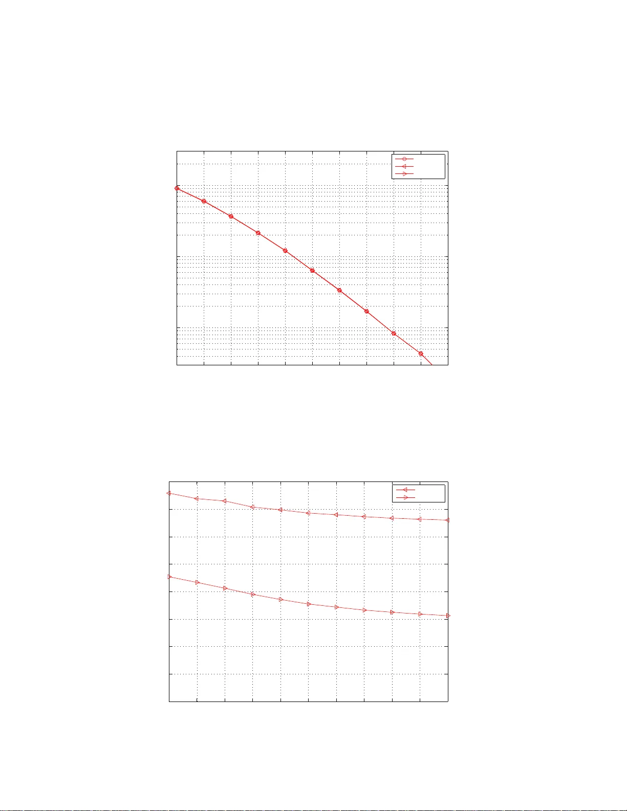
Rotated and Scaled Alamo uti Co ding F rans M.J. Willems ∗ Octob er 30, 2018 Abstract Rep etition-based retransmission is used in Alamouti-mo dulation [1998] for 2 × 2 MIMO sys- tems. W e prop ose to use instead of ordinary rep etition so-called ”scaled rep etition” together with rotation. It is sho wn that the rotated and scaled Alamouti cod e has a hard-decision p erformance w hich is only slightl y w orse than that of the Golden code [2005], the b est know n 2 × 2 space-time code. Decod ing the Golden co de requires an exhaustive search o ver a ll codewords, while our rotated and scaled A lamouti code can be deco ded with an acceptable complexity ho wev er. 1 Scaled-rep etition Retransmission for the SISO Ch annel First we consider transmission over a single-input s ingle-output (SISO) additive white Gaus s ian noise (A W GN) channel (see Fig. 1 ), and in tro duce scaled-r epe titio n retransmiss ion. It turns out that scaled-r ep etition improv es up on or dinary-rep etition retrans mission. 1.1 Some information theory ✗ ✖ ✔ ✕ ✲ ✲ ❄ receiver transmitter n y x + Figure 1: The A W GN channel. The real-v a lued output y k for transmissio n k = 1 , 2 , · · · , K , see Fig. 1, s atisfies y k = x k + n k , (1) where x k is the real-v alued channel input for trans mis s ion k and n k is a real-v a lued Gaussia n noise sample with mea n E [ N k ] = 0 , v a riance E [ N 2 k ] = σ 2 , which is uncorrelated with a ll other noise samples. The transmitter p ow er is limited, i.e. w e require that E [ X 2 k ] ≤ P . It is well-known that an X which is Ga ussian with mean 0 and v ariance P ac hieves capa cit y . This basic capacity (in bit/transm.) equals C = 1 2 log 2 (1 + P σ 2 ) . (2) When we retransmit (rep eat) co dewords , each symbol x k from such a co deword ( x 1 , x 2 , · · · , x K ) is actually transmitted and received twice, i.e. x k 1 = x k 2 = x k , and y k 1 = x k + n k 1 , and y k 2 = x k + n k 2 . (3) ∗ Philips Researc h Lab oratories, High T ech C ampus 37, 5656AE Eindho ve n, The Nethe rlands 1 ✄ ✂  ✁ ✄ ✂  ✁ ✄ ✂  ✁ ✄ ✂  ✁ ✄ ✂  ✁ ✄ ✂  ✁ ✄ ✂  ✁ ✄ ✂  ✁ +3 +3 +1 +1 -1 -1 -3 -3 -3 -1 +1 +3 -3 x k 2 x k 2 x k 1 x k 1 +3 -1 +1 Figure 2: Two ma pping s from x k 1 to x k 2 . On the right the sca led-rep etition mapping, left the ordinary - rep etition mapping . An optimal receiv er can for m z k = y k 1 + y k 2 2 = x k + n k 1 + n k 2 2 . Now the v ar iance o f the noise v a riable ( N k 1 + N k 2 ) / 2 is σ 2 / 2. Ther efore the rep etition ca pacity for a single r ep etition in bit/tra nsm. is C r = 1 4 log 2 (1 + 2 P σ 2 ) . (4) Fig. 3 shows the basic ca pacity C (black line) and rep etition ca pacity C r (blue line) a s a function of the sig nal-to-nois e ratio SNR which is defined as SNR ∆ = P /σ 2 . (5) It is easy to see that alwa y s C r ≤ C . F or large SNR w e ma y write C r ≈ C / 2 + 1 / 4, while for sma ll SNR we obtain C r ≈ C . 1.2 Ordinary and scaled repetit ion for 4-P AM When we use 4-P AM mo dulation, the channel inputs x k assume v a lues from A 4-P AM = {− 3 , − 1 , +1 , +3 } , each with proba bilit y 1 / 4. Or dinary repetitio n, see (3 ), leads to signal points ( x 1 , x 2 ) = ( x, x ) for x ∈ A 4-P AM , see the left part o f Fig. 2. F or this case the maximum transmissio n rate I ( X ; Y 1 , Y 2 ) is shown in Fig. 3 with blue aster isks. Note that this maximum tr a nsmission rate is s lightly smaller than the cor resp onding capa cities C r , ma inly b ecause uniform inputs are used instead of Gauss ia ns. W e can use Be ne lli’s [3] metho d to improv e up on ordinar y-rep etition re tr ansmission, i.e. by mo dulating the retra nsmitted symbol differently . W e could e.g. tak e x k 1 = x k , a nd x k 2 = M 2 ( x k ) for x k ∈ A 4-P AM , (6) where M 2 ( α ) = 2 α − 5 if α > 0 and M 2 ( α ) = 2 α + 5 for α < 0. W e call this metho d sc ale d r ep et ition since w e s c ale a symbol b y a facto r (2 here) and then comp ensate (add - 5 or +5) in order to obtain a symbol from A 4-P AM . This results in the signal points ( x, M 2 ( x )) for x ∈ A 4-P AM , see Fig. 2, righ t part. Also for the scaled-r e petition ca se the maxim um tra ns mission r ate I ( X ; Y 1 , Y 2 ) is shown in fig ure 3, no w with red asterisk s. Note that this ma x im um transmissio n rate is only slig h tly smaller than the basic capacity C. Or dinary rep etition is how ever definitively inferior to the basic transmission if the SNR is not very sma ll. 1.3 Demo dulation complexit y Scaled rep etition outper fo rms o r dinary rep e tition, but also has a disadv a n tage. In an ordinary- rep etition sy s tem the o utput y k = ( y k 1 + y k 2 ) / 2 is simply sliced. In a system tha t uses scaled rep etition we can only slice after having distinguished b etw een tw o ca ses. More precisely note that x k 2 = M 2 ( x k ) = 2 x k − D 2 ( x k ), wher e D 2 ( α ) = 5 if α > 0 and D 2 ( α ) = − 5 if α < 0. Now w e can use a slicer for y k 1 + 2 y k 2 = x k + n k 1 + 2(2 x k − D 2 ( x k ) + n k 2 ) = 5 x k − 2 D 2 ( x k ) + n k 1 + 2 n k 2 . Assuming that x k ∈ { − 3 , − 1 } we get that D 2 ( x k ) = − 5 and this implies that we s hould put a 2 −15 −10 −5 0 5 10 15 0 0.5 1 1.5 Figure 3: Basic capa city C (black curve) a nd rep etition capacity C r (blue) in bit/tr ansm. as a function of SNR = P /σ 2 in dB (horizontally). Also the maximum transmission rates a chiev able with 4-P AM in the ordina ry-rep etition case (blue *’s). In red *’s the maxim um rates achiev able using scaled-r epe titio n mapping . threshold at 0 to dis tinguish b etw ee n − 3 a nd − 1. Similarly assuming that x k ∈ { + 1 , + 3 } we get D 2 ( x k ) = 5 and we must slice y k 1 + 2 y k 2 again with a threshold a t 0 . Then the b est overall candidate ˆ x k is found by minimizing ( y k 1 − ˆ x k ) 2 + ( y k 2 − M 2 ( ˆ x k )) 2 ov e r the tw o candidates. 2 F undamen tal Prop erties for the 2 × 2 MIMO Chann el 2.1 Mo del description ✓ ✒ ✏ ✑ ✓ ✒ ✏ ✑ ✟ ✟ ✟ ✟ ✟ ✟ ✟ ✟ ✟ ❍ ❍ ❍ ❍ ❍ ❍ ❍ ❍ ❍ ✲ ✲ ❄ ❄ Rec. T r. h 11 h 22 h 21 h 12 x 1 x 2 + + y 1 y 2 n 1 n 2 Figure 4: Mo de l of a 2 × 2 MIMO channel. Next co nsider a 2 × 2 MIMO channel (see Fig. 4). Both the transmitter and the receiver use t wo a ntenn as. The output v ector ( y 1 k , y 2 k ) at transmission k rela tes to the cor resp onding input vector ( x 1 k , x 2 k ) as given by  y 1 k y 2 k  =  h 11 h 12 h 21 h 22   x 1 k x 2 k  +  n 1 k n 2 k  (7) where ( N 1 k , N 2 k ) is a pair of independent zero-mean circular ly symmetric complex Ga ussians, bo th having v aria nce σ 2 (per tw o dimensions). Noise v a riable pairs in different tr ansmissions are independent. 3 W e assume that the four channel co e fficie n ts H 11 , H 12 , H 21 , a nd H 22 are independent zer o- mean cir cularly symmetric complex Gaussia ns, each ha ving v a riance 1 (p er tw o dimensions ). Th e channel c o efficients ar e chosen prior to a blo ck of K tr ansmissions and r emain c onstant over that blo ck. The complex transmitted sy m b ols ( X k 1 , X k 2 ) must satisfy a power constraint, i.e. E [ X k 1 X ∗ k 1 + X k 2 X ∗ k 2 ] ≤ P . (8) 2.2 T elatar capacit y If the ch annel input v aria bles are independent zero-mean circularly symmetric complex Gaussians bo th having v aria nc e P / 2 , then the resulting m utual infor mation (called T elatar capacity here, see [5]) is 1 C T elatar ( H ) = log 2 det( I 2 + P / 2 σ 2 H H † ) , (9) where H =  h 11 h 12 h 21 h 22  , i.e. the actual channel-coefficient matrix and I 2 the 2 × 2 identit y matrix. Also in the 2 × 2 MIMO case we define the signal-to- niose ratio a s SNR ∆ = P /σ 2 . (10) It can b e shown (see e.g. Y ao ([6], p. 36) that for fixed R and SNR larg e enough Pr { C T elatar( H ) < R } ≈ γ · SNR − 4 , for some co nstant γ . 2.3 W orst -case er ror-probabilities Consider M (one for each message) K × 2 co de-matrices c 1 , c 2 , · · · , c M resulting in a unit av er age energy co de. Then T arokh, Seshadri and Calder bank [4] show ed that for large SNR Pr { c → c ′ } ≈ γ ′ (det(( c ′ − c )( c ′ − c ) † ) − 2 SNR − 4 . (11) for some γ ′ if the r ank o f the difference matric e s c − c ′ is 2, and w e transmit x = √ P c . If this holds for all differe nce matrices w e say tha t the diversit y order is 4. Therefore it makes sense to maximize the minimum mo dulus of the determina nt ov er all co de- matrix differences. 3 Alamouti: Ordinary Rep etition Alamouti [1] prop osed a mo dulation scheme (space-time co de) for the 2 × 2 MIMO ca nnel which allows for a very simple detector. Two complex symbols s 1 and s 2 are tra ns mitted in the first transmission (an o dd tra nsmission) and in the second tr ansmission (the next even transmission) these symbols are mo r e or less rep ea ted. More prec isely  x 11 x 12 x 21 x 22  =  s 1 − s ∗ 2 s 2 s ∗ 1  . (12) The received signa l is now  y 11 y 12 y 21 y 22  =  h 11 h 12 h 21 h 22   s 1 − s ∗ 2 s 2 s ∗ 1  +  n 11 n 12 n 21 n 22  . (13) Rewriting this res ults in     y 11 y 21 y ∗ 12 y ∗ 22     =     h 11 h 12 h 21 h 22 h ∗ 12 − h ∗ 11 h ∗ 22 − h ∗ 21      s 1 s 2  +     n 11 n 21 n ∗ 12 n ∗ 22     , (14) 1 Here H † denotes the Hermi tian transp ose of H . It i nv olves b oth transp osition and complex conjugation. 4 or more compactly y = s 1 a + s 2 b + n, with y = ( y 11 , y 21 , y ∗ 12 , y ∗ 22 ) T , a = ( h 11 , h 21 , h ∗ 12 , h ∗ 22 ) T , b = ( h 12 , h 22 , − h ∗ 11 , − h ∗ 21 ) T , and n = ( n 11 , n 21 , n ∗ 12 , n ∗ 22 ) T . (15) Since a and b are orthogo nal the symbol estimates ˆ s 1 and ˆ s 2 can b e determined by simply slicing ( a † y ) / ( a † a ) and ( y † b ) / ( b † b ) resp ectively . Another adv antage of the Alamouti metho d is that the densities o f a † a and b † b are (identical and) chi-square with 8 degrees of freedo m. This r esults in a diversity order 4, i.e. Pr { d ( S 1 , S 2 ) 6 = ( S 1 , S 2 ) } ≈ γ ′′ · SNR − 4 , (16) for fixed ra te and large enough SNR. A disadv antage of the Alamo uti metho d is that only tw o complex sym b ols are transmitted ev ery t wo trans missions, but mor e-imp ortantly that the sym bo ls transmitted in the second transmission are more or less r ep etitions of the symbols in the first transmissio n. Section 1 how ever sugges ts that we can improve upon ordinary rep etition. 4 The rotated and scaled Alamouti metho d 4.1 Metho d description Having seen in section 1 that scaled-rep etition improv es upo n o r dinary rep etition in the SISO case, we use this concept to improv e upon the standard Alamouti sc heme for MIMO transmissio n. Instead of just rep eating the s ymbols in the second transmiss ion w e sc a le them. More precisely , when s 1 and s 2 are elements of A 16-QAM ∆ = { a + j b | a ∈ A 4-P AM , b ∈ A 4-P AM } , we could transmit for some v alue of θ the signals  x 11 x 12 x 21 x 22  =  s 1 · exp( j θ ) − s ∗ 2 M 2 ( s 2 ) M 2 ( s ∗ 1 )  =  s 1 · exp( j θ ) − s ∗ 2 2 s 2 2 s ∗ 1  −  0 0 D 2 ( s 2 ) D 2 ( s ∗ 1 )  , (17) where M 2 ( α ) = 2 α − D 2 ( α ) with D 2 ( α ) = 5 β when β is the complex sign of α . A first questio n is to deter mine a g o o d v alue for θ . Therefor e we determine for 0 ≤ θ ≤ π / 2 the minimum mo dulus o f the determinant mindet ( θ ) mindet( θ ) = min ( s 1 ,s 2 ) , ( s ′ 1 ,s ′ 2 ) | det( X ( s 1 , s 2 , θ ) − X ( s ′ 1 , s ′ 2 , θ )) | , (18) where X =  x 11 x 12 x 21 x 22  is the co de matrix. The minimum mo dulus o f the determinant as a function of θ c an b e found in Fig . 5. The maxim um v alue of the minimum determinant (i.e. 7.613) o ccurs for θ opt. = 1 . 028 . (19) W e will use this v alue for θ in what follows. 5 0 0.5 1 1.5 0 1 2 3 4 5 6 7 8 Minimum Determinant, 16QAM−codesymbols, R=4 bits/transm. Figure 5: Minimum mo dulus of the determinant for rota ted and scaled Alamouti as a function o f θ horizontally . 4.2 Hard-decision P erformance W e hav e co mpared the message-error -rate for several R = 4 space- time codes in Fig. 6. By message-e rror- rate we mean the pr obability Pr { b X 6 = X } . Note that for each ”test” we generate a new messag e (8-bit) and a new channel matrix. The deco der is optimal for all co des, it p erforms M L - deco ding (exha ustive sear ch). The metho ds that we hav e co nsidered are: 1. Uncode d , in green. W e transmit X =  x 11 x 12 x 21 x 22  , (20) where x 11 , x 12 , x 21 , and x 22 are symbols fro m A 4-QAM . 2. Alamouti , in blue, see (12), where s 1 and s 2 are symbols from A 16-QAM . 3. Tilted QAM , in cyan. Prop osed by Y ao and W ornell [7]. Let s a , s b , s c , and s d symbols from A 4-QAM . Then we transmit  x 11 x 22  =  cos( θ 1 ) − sin( θ 1 ) sin( θ 1 ) cos( θ 1 )   s a s b  ,  x 21 x 12  =  cos( θ 2 ) − sin( θ 2 ) sin( θ 2 ) cos( θ 2 )   s c s d  , (21) for θ 1 = 1 2 arctan( 1 2 ) and θ 2 = 1 2 arctan(2). 4. Rotated and sca led Alamouti , in red, s ee (17) fo r θ = 1 . 028, and with s 1 and s 2 from A 16-QAM . 5. Golden co de , in magenta. Pr op osed b y Belfio re et al. [2 ]. No w X = 1 √ 5  α ( z 1 + z 2 θ ) α ( z 3 + z 4 θ ) j · α ( z 3 + z 4 θ ) α ( z 1 + z 2 θ )  , (22) with θ = 1+ √ 5 2 , θ = 1 − √ 5 2 , α = 1 + j − j θ , and α = 1 + j − j θ and where z 1 , z 2 , z 3 , and z 4 are A 4-QAM -symbols. 6 10 11 12 13 14 15 16 17 18 19 20 10 −3 10 −2 10 −1 MER, 16QAM code−symbols, R=4 bits/transm., 1000 errors Telatar uncoded Alamouti Rot.Scal.Rep. Tilted QAM Golden Code Figure 6: Mes sage error ra te fo r several R=4 spac e -time co des. 6. T el atar , in black. This is the pr obability that the T elatar capacity of the c hannel is smaller than 4. Clearly it follows from Fig. 6 that the winner is the Golden co de. Ho wev er rotated and sca led Alamouti is only slightly worse, roughly 0 . 2 dB. Imp or tant is that Alamouti co ding is roug hly 2 dB worse than the Go lden co de. 5 Deco ding complexit y Clearly the Golden co de is b etter than rotated and s caled Alamo uti. Ho wev e r the Golden co de in pr inc iple req uir es the deco der to chec k a ll 2 5 6 alternative co dewords. Here w e will inv estigate the co mplexit y and p er formance of a sub opti mal rotated and scaled Alamouti deco der. Denote Θ = exp( j θ opt. ). A. In the rota ted a nd scaled Ala mouti case the received vector is     y 11 y 21 y ∗ 12 y ∗ 22     =     h 11 Θ 2 h 12 h 21 Θ 2 h 22 2 h ∗ 12 − h ∗ 11 2 h ∗ 22 − h ∗ 21      s 1 s 2  (23) −     0 0 h ∗ 12 h ∗ 22     D 2 ( s 1 ) −     h 12 h 22 0 0     D 2 ( s 2 ) +     n 11 n 21 n ∗ 12 n ∗ 22     . 7 W e can wr ite this as y = s 1 a + s 2 b − D 2 ( s 1 ) c − D 2 ( s 2 ) d + n, y = ( y 11 , y 21 , y ∗ 12 , y ∗ 22 ) T , a = ( h 11 Θ , h 21 Θ , 2 h ∗ 12 , 2 h ∗ 22 ) T , b = (2 h 12 , 2 h 22 , − h ∗ 11 , − h ∗ 21 ) T , c = (0 , 0 , h ∗ 12 , h ∗ 22 ) T , d = ( h 12 , h 22 , 0 , 0) T , and n = ( n 11 , n 21 , n ∗ 12 , n ∗ 22 ) T . F or the co s( φ ) of the angle b etw een a and b we ca n wr ite cos( φ ) = | 2(Θ − 1)( h 11 h ∗ 12 + h 21 h ∗ 22 )] | h 11 | 2 + | h 21 | 2 + 4 | h 12 | 2 + 4 | h 22 | 2 . (24) B. Instead of deco ding ( s 1 , s 2 ) we can also deco de ( t 1 , t 2 ) = ( M 2 ( s 1 ) , M 2 ( s 2 )) which is equiv alent to ( s 1 , s 2 ). Ther efore we rewr ite (1 7) and obtain  x 11 x 12 x 21 x 22  =  − M 2 ( t 1 )Θ M 2 ( t ∗ 2 ) t 2 t ∗ 1  =  − 2 t 1 Θ 2 t ∗ 2 t 2 t ∗ 1  −  − D 2 ( t 1 )Θ D 2 ( t ∗ 2 ) 0 0  , (25) since t = M 2 ( s ) implies that s = − M 2 ( t ). Now     y 11 y 21 y ∗ 12 y ∗ 22     =     − 2 h 11 Θ h 12 − 2 h 21 Θ h 22 h ∗ 12 2 h ∗ 11 h ∗ 22 2 h ∗ 21      t 1 t 2  (26) −     − h 11 Θ − h 21 Θ 0 0     D 2 ( t 1 ) −     0 0 h ∗ 11 h ∗ 21     D 2 ( t 2 ) +     n 11 n 21 n ∗ 12 n ∗ 22     . W e can wr ite this as y = t 1 a ′ + t 2 b ′ − D 2 ( t 1 ) c ′ − D 2 ( t 2 ) d ′ + n , a ′ = ( − 2 h 11 Θ , − 2 h 21 Θ , h ∗ 12 , h ∗ 22 ) T , b ′ = ( h 12 , h 22 , 2 h ∗ 11 , 2 h ∗ 21 ) T , c ′ = ( − h 11 Θ , − h 21 Θ , 0 , 0) T , and d ′ = (0 , 0 , h ∗ 11 , h ∗ 21 , 0 , 0) T , and for the cos( φ ′ ) of the angle b etw een a ′ and b ′ we can wr ite cos( φ ′ ) = | 2(Θ − 1 )( h 11 h ∗ 12 + h 21 h ∗ 22 ) | 4 | h 11 | 2 + 4 | h 21 | 2 + | h 12 | 2 + | h 22 | 2 . (27) C. It now fo llows fr om the inequality 2 r 1 r 2 ≤ r 2 1 + r 2 2 (where r 1 and r 2 are reals), that cos( φ ) ≤ | Θ − 1 | · | h 11 | 2 + | h 12 | 2 + | h 21 | 2 + | h 22 | 2 | h 11 | 2 + | h 21 | 2 + 4 | h 12 | 2 + 4 | h 22 | 2 , cos( φ ′ ) ≤ | Θ − 1 | · | h 11 | 2 + | h 12 | 2 + | h 21 | 2 + | h 22 | 2 4 | h 11 | 2 + 4 | h 21 | 2 + | h 12 | 2 + | h 22 | 2 . (28) 8 If | h 12 | 2 + | h 22 | 2 ≥ | h 11 | 2 + | h 21 | 2 , (29) then cos( φ ) ≤ 2 | Θ − 1 | 5 = 0 . 3 93, e ls e co s( φ ′ ) ≤ 2 | Θ − 1 | 5 = 0 . 3 93. Ther efore it makes sense to dec o de ( s 1 , s 2 ) when (29) ho lds and ( t 1 , t 2 ) when (29) do e s not hold. Using ze r o-forcing to deco de, the noise enhancement is then at mo st 1 / (1 − 0 . 393 2 ) = 1 . 183 which is 0 .729 dB. W e s hall see la ter that noise enhancement tur ns out to b e un-no ticeable in pra c tis e . D. The deco ding pro cedure is straig ht forward. F o cus on the ca se where we deco de ( s 1 , s 2 ) for a moment. F or all 16 alternatives of ( D 2 ( s 1 ) , D 2 ( s 2 )) the vector z = y + D 2 ( s 1 ) c + D 2 ( s 2 ) d = s 1 a + s 2 b + n (30) and is determined. Then compute the sufficient sta tistic  a † z b † z  =  a † a a † b b † a b † b   s 1 s 2  +  a † n b † n  . (31) Next us e the in verted matrix M =  b † b − a † b − b † a a † a  /D wher e D = ( a † a )( b † b ) − ( b † a )( a † b ) to obtain  ˜ s 1 ˜ s 2  = M  a † z b † z  . Next bo th ˜ s 1 and ˜ s 2 are sliced under the r estriction that o nly alternatives that match the assumed v a lues D 2 ( s 1 ) a nd D 2 ( s 2 ) are p oss ible o utcomes. This is done for all 1 6 alter natives ( D 2 ( s 1 ) , D 2 ( s 2 )). The b est result in terms o f Euclidea n distance is now chosen. In c onsidering a ll a lternatives ( D 2 ( s 1 ) , D 2 ( s 2 )) we o nly need to slice when the length of z − ˜ s 1 a − ˜ s 2 b is s ma ller than the close s t distance we have observed so far . This reduces the num b er of slicing steps. W e call this approach METHOD 1. E. The num b er of slicing steps can ev en b e further decreased if we start slicing with the most promising alterna tive ( D 2 ( s 1 ) , D 2 ( s 2 )). This approa ch is calle d METHOD 2. Ther efore we note tha t the ”direct” s 1 -signal-co mpo nent in X is  s 1 Θ 0 0 − s ∗ 1 / 2  . Therefore w e can slice ( e † 1 y ) / ( e † 1 e 1 ) in o rder to find a go o d gues s for D 2 ( s 1 ). Similarly we slic e ( e † 2 y ) / ( e † 2 e 2 ) to find a go o d first guess for D 2 ( s 2 ). Here e 1 = ( h 11 Θ , h 21 Θ , − h ∗ 12 / 2 , − h ∗ 22 / 2) T , (32) e 2 = ( − h 12 / 2 , − h 22 / 2 , − h ∗ 11 , − h ∗ 21 ) T . (33) Then w e consider the other 15 alternatives and only slice if necessary . Note that s imilar metho ds apply if we w ant to deco de ( t 1 , t 2 ). F. W e have carried out simulations, first to find o ut what the degr adation of the sub optimal deco ders acco rding to metho d 1 and metho d2 is relative to ML-deco ding. The result is shown in Fig. 7. Conclusion is that the suboptimal deco ders do not demonstrate a p erforma nce degrada tio n. W e hav e also considered the num b er of slicings for b o th metho d 1 and method 2. This is shown in Fig. 8. It can b e observed that method 1 leads to roughly 7 slicing s (as o ppo sed to 16). Metho d 1 further decr eases the num b er o f slicing to roughly 3.5. 6 Conclusion Rotated a nd s caled Alamo uti has a hard-decision p erfor mance whic h is only slightly worse than that of the Golden co de, but can b e deco ded w ith an acc eptable complexity . W e finally r emark that we hav e obtained similar r esults for co des based o n ma pping M 3 ( · ) for 9 -P AM. 9 10 11 12 13 14 15 16 17 18 19 20 10 −3 10 −2 10 −1 MER, Rot.Scal.Alam., 16QAM code−symbols, R=4 bits/transm., 1000 errors full search method 1 method2 Figure 7: Message e r ror r ate for three Rotated Sca led Alamouti deco der s ( R = 4), horizontally SNR. 10 11 12 13 14 15 16 17 18 19 20 0 1 2 3 4 5 6 7 8 Av.nr. slicings, Rot.Scal.Alam., 16QAM code−symbols, R=4 bits/transm., 1000 errors method 1 method2 Figure 8: Num b er o f slicing s for tw o Ro tated Sclaed Alamouti deco der s ( R = 4), horizontally SNR. 10 References [1] S.M. Alamouti, ”A simple transmit diversit y techn ique for wireless communications,” IEEE J. S el. A r e as. Comm. vol. 16, pp. 1451-1 458, Octob er 1998 . [2] J.-C. Belfiore, G. Rek aya, E. Viterbo , ”The golden co de: A 2 × 2 full-rate space-time c o de with nonv anishin determinants,” IEEE T r ans. Inform. The ory, vol. IT-5 1, No. 4, pp. 1 432 - 1436, April 200 5 . [3] G. Benelli, ” A new metho d fo r the integration of mo dula tion and channel co ding in a n ARQ proto col,” IEEE T r ans. Commun., vol. COM-40, pp. 159 4 - 1 606, O ctob er 1992 . [4] V. T a rokh, N. Seshadri, and A.R. Calderbank, ”Space-Time Codes for High Data Rate Wire- less Commun ication: Performance Criterio n a nd Co de Co nstruction,” IEEE T r ans. In form. The ory, V ol. 44, pp. 74 4- 7 65, March 1998. [5] I.E. T elatar , ”Capacity of multi-antenna Gaussian channels” Eur op e an T r ans. T ele c ommun i- c ations, vol. 10 , pp. 58 5-595 , 1999 . (Originally published as A T& T T echnical Memorandum, 1995). [6] H. Y ao, ” Efficient Sig na l, Co de, and Receiver Designs for MIMO Communication Systems,” Ph.D. thesis, M.I.T., J une 200 3 . [7] H. Y a o and G.W. W o rnell, ”Ac hiev ing the full MIMO div ersity-m ultiplexing frontier with rotation-ba sed space- time co des,” in Pr o c. Al lerton Conf. Commun. Contr ol, and Comput. , Monticello, IL, Oct. 2003. 11