Capacity Bounds for Peak-Constrained Multiantenna Wideband Channels

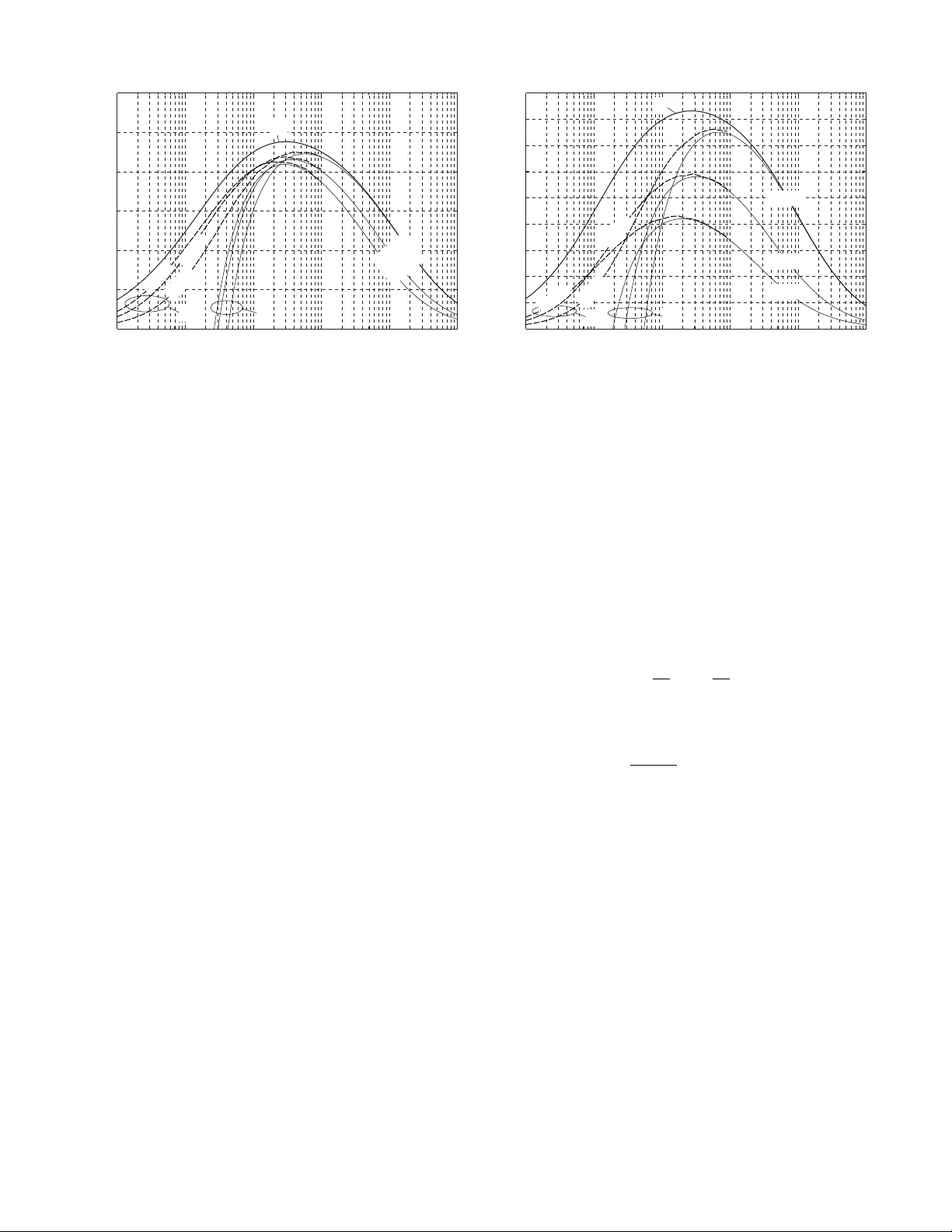
1 Capacity Bounds for Peak-Constrained Multiantenna W ideband Channels Ulrich G. Schuster , Student Member , IEEE , Giuseppe Durisi, Member , IEEE , Helmut B ¨ olcskei, Senior Member , IEEE , and H. V incent Poor , F ellow , IEEE Abstract —W e deriv e bounds on the noncoherent capacity of a very general class of multiple-input multiple-output channels that allow for selectivity in time and frequency as well as f or spatial cor - relation. The bounds apply to peak-constrained inputs; they are explicit in the channel’ s scattering function, are useful f or a large range of bandwidth, and allow to coarsely identify the capacity- optimal combination of bandwidth and number of transmit an- tennas. Furthermore, we obtain a closed-form expression for the first-order T aylor series expansion of capacity in the limit of in- finite bandwidth. From this expression, we conclude that in the wideband regime: (i) it is optimal to use only one transmit antenna when the channel is spatially uncorr elated; (ii) rank-one statistical beamforming is optimal if the channel is spatially correlated; and (iii) spatial correlation, be it at the transmitter , the r eceiver , or both, is beneficial. Index T erms —Noncoherent capacity , MIMO systems, under - spread channels, wideband channels. I . I N T RO D U C T I O N A N D S U M M A RY O F R E S U LT S Bandwidth and space are sources of degrees of freedom that can be utilized to transmit information ov er wireless fading channels. Channel measurements indicate that an increase in the number of degrees of freedom also increases the channel uncertainty that the receiv er has to resolve [1]. If the transmit signal is allowed to be peaky , that is, if it can ha ve an unbounded peak value, channel uncertainty is immaterial in the limit of infinite bandwidth. Indeed, for a fairly general class of fading channels, the capacity of the infinite-bandwidth additive white Gaussian noise (A WGN) channel can be achiev ed [2]–[4]. A more realistic modeling assumption is to limit the peak power of the transmitted signal. In this case, the capacity be- havior of most channels changes drastically: for certain types of peak constraints, the capacity can even approach zero in the wideband limit [3], [5], [6]. Intuitively , under a peak con- straint on the transmit signal, the receiv er is no longer able to resolv e the channel uncertainty as the number of de grees of freedom increases. Consequently , questions of significant practical relev ance are ho w much bandwidth to use and whether This work was supported partly by the European Commission through the Integrated Project P U L S ER S Phase II under contract No. FP6-027142 and partly by the U. S. National Science Foundation under Grants ANI-03-38807 and CNS-06-25637. Part of this work originated while U. G. Schuster was a visiting researcher at Princeton University . A conference version of this paper has been submitted to the IEEE Int. Symposium on Information Theory (ISIT), T oronto, Canada, July 2007. U. G. Schuster , G. Durisi, and H. B ¨ olcskei are with the Communication T ech- nology Laboratory , ETH Zurich, 8092 Zurich, Switzerland (e-mail: { schuster , gdurisi, boelcskei } @nari.ee.ethz.ch). H. V . Poor is with Princeton University , Princeton, NJ 08544, U.S.A. (e-mail: poor@princeton.edu). spatial degrees of freedom obtained by multiple antennas can be exploited to increase capacity . The aim of this paper is to characterize the capacity of spa- tially correlated multiple-input multiple-output (MIMO) fading channels that are time and frequency selectiv e, i.e., that exhibit memory in frequency and time, gi ven that (i) the transmit signal has bounded peak po wer and (ii) the transmitter and the recei ver know the channel law but both are ignorant of the channel realization. The assumptions (ii) constitute the noncoher ent setting , as opposed to the coherent setting where the receiv er has perfect channel state information (CSI) and the transmitter knows the channel law only . Related W ork: Sethuraman et al. [7] analyzed the capacity of peak-constrained MIMO Rayleigh-fading channels that are frequency flat, time selectiv e, and spatially uncorrelated and deriv ed an upper bound and a low-SNR lo wer bound that allow to characterize the second-order T aylor series expansion of capacity around the point SNR = 0 . In particular, it is shown in [7] that in the low-SNR re gime it is optimal to use only a single transmit antenna, while additional receiv e antennas are always beneficial. The low-SNR results also apply to a wideband channel with fixed total transmit power and increasing bandwidth if the wideband channel can be decomposed into a set of independent and identically distributed (i.i.d.) parallel subchannels in frequency [7]. Spatial correlation is often beneficial in the noncoherent set- ting. For the separable (Kronecker) spatial correlation model [8], [9], Jafar and Goldsmith [10] prov ed that transmit correlation increases the capacity of a memoryless fading channel. Moreov er , in the low-SNR regime, the rates achiev able with on-off keying on memoryless fading channels [11] and with finite-cardinality constellations on block-fading channels [12] increase in the presence of spatial correlation at the transmitter , the recei ver , or both. Contributions: W e consider a point-to-point MIMO channel model where each component channel between a given trans- mit antenna and a gi ven recei ve antenna is underspr ead [13] and satisfies the standard wide-sense stationary uncorrelated- scattering (WSSUS) assumption [14]; hence, our channel model allows for selectivity in time and frequency . W e assume that the component channels are spatially correlated according to the sep- arable correlation model [8], [9] and that they are characterized by the same scattering function; furthermore, the transmit signal is peak constrained. On the basis of a discrete-time, discrete- frequency approximation of said channel model that is enabled by the underspread property [15], we obtain the following results: 2 • W e derive upper and lower bounds on capacity . These bounds are explicit in the channel’ s scattering function and allow to coarsely identify the capacity-optimal combination of bandwidth and number of transmit antennas for a fixed number of receive antennas. • For spatially uncorrelated channels, we generalize the asymptotic results of Sethuraman et al. [7] to time- and frequency-selecti ve channels: for large enough bandwidth— or equiv alently , for small enough SNR—it is optimal to use a single transmit antenna only , while additional recei ve antennas always increase capacity . • Differently from the coherent setting [16]–[18], we find that both transmit and receive correlation are beneficial in the wideband regime. Furthermore, rank-one statistical beamforming along the strongest eigenmode of the spatial transmit correlation matrix is optimal for large bandwidth. As the deri vations of the results in the present paper rely on several techniques dev eloped in [19] for single-input single- output (SISO) time- and frequency-selecti ve channels, we detail only the new elements in our deri vations and refer to [19] otherwise. Notation: Uppercase boldface letters denote matrices and lowercase boldf ace letters designate vectors. The superscripts T , ∗ , and H stand for transposition, element-wise conjugation, and Hermitian transposition, respectiv ely . F or tw o matrices A and B of appropriate dimensions, the Hadamard product is denoted as A  B and the Kronecker product is denoted as A ⊗ B ; to simplify notation, we use the con vention that the ordinary matrix product always precedes the Kronecker and Hadamard products, e.g., AB  C means ( AB )  C for some matrix C of appropriate dimension. W e designate the identity matrix and the all-zero matrix of dimension N × N by I N and 0 N , respectiv ely; D 1 / 2 is the unique nonnegati ve definite square-root matrix of the nonne gativ e definite matrix D . The determinant of a square matrix X is det( X ) , its rank is rank( X ) , and its trace is tr( X ) . The vector of eigenv alues of X is denoted by λ ( X ) , W e let diag { x } denote a diagonal square matrix whose main diagonal contains the elements of the vector x . The function δ ( x ) is the Dirac distribution. All logarithms are to the base e . For two functions f ( x ) and g ( x ) , the notation f ( x ) = o ( g ( x )) means that lim x → 0 f ( x ) /g ( x ) = 0 . If two random variables a and b follow the same distribution, we write a ∼ b . Finally , we denote the expectation operator by E [ · ] and the Fourier transform operator by F [ · ] . I I . S Y S T E M M O D E L In the following subsections, we first introduce the SISO model for one component channel and subsequently discuss the extension of this model to the MIMO setting. A. Underspr ead WSSUS Channels The relation between the input signal x ( t ) and the corre- sponding output signal y ( t ) of a SISO stochastic linear time- varying (L TV) channel H can be expressed as y ( t ) =  H x  ( t ) + w ( t ) = Z t 0 k H ( t, t 0 ) x ( t 0 ) dt 0 + w ( t ) (1) where k H ( t, t 0 ) denotes the random kernel of the channel opera- tor H and w ( t ) is a white Gaussian noise process. W e assume that k H ( t, t 0 ) is a zero-mean jointly proper Gaussian (JPG) process in t and t 0 whose Fourier transforms are well defined. In particular, L H ( t, f ) = F τ → f [ k H ( t, t − τ )] is called the time- varying transfer function and S H ( ν, τ ) = F t → ν [ k H ( t, t − τ )] is called the spr eading function . W e assume that the channel is WSSUS, so that E [ S H ( ν, τ ) S ∗ H ( ν 0 , τ 0 )] = C H ( ν, τ ) δ ( ν − ν 0 ) δ ( τ − τ 0 ) . Consequently , the statistical properties of the channel H are completely specified through its so-called scattering func- tion C H ( ν, τ ) . A WSSUS channel is said to be underspr ead [15] if C H ( ν, τ ) is compactly supported on a rectangle [ − ν 0 , ν 0 ] × [ − τ 0 , τ 0 ] whose spr ead ∆ H = 4 ν 0 τ 0 satisfies ∆ H < 1 . B. Discrete Appr oximation T o simplify information-theoretic analysis, we would like to diagonalize the channel operator H , i.e., replace the integral input-output (IO) relation (1) by a countable set of scalar IO relations. T o this end, we cannot use an eigendecomposition of the random kernel k H ( t, t 0 ) because its eigenfunctions are random as well, and hence unknown to the transmitter and the receiver in the noncoherent setting. Y et, for underspread channels it is possible to find an orthonormal set of deter- ministic approximate eigenfunctions that depend only on the channel’ s scattering function [15]. Consequently , knowledge of the channel law—and hence of the scattering function—is sufficient for transmitter and receiver to approximately diago- nalize H . One possible choice of approximate eigenfunctions is the W eyl-Heisenber g set of mutually orthogonal time-frequency shifts g k,n ( t ) = g ( t − k T ) e i 2 π nF t of some prototype func- tion g ( t ) that is well localized in time and frequency . The grid parameters T and F need to satisfy T F ≥ 1 ; then, the kernel of H can be approximated as [19] k H ( t, t 0 ) ≈ ∞ X k = −∞ ∞ X n = −∞ L H ( k T , nF ) | {z } h [ k,n ] g k,n ( t ) g ∗ k,n ( t 0 ) . (2) The approximation quality depends on the prototype func- tion g ( t ) and on the parameters T and F , which need to be suit- ably chosen with respect to the scattering function C H ( ν, τ ) [15], [19]. The eigen values of the approximate channel with ker- nel (2) are gi ven by h [ k , n ] = L H ( k T , nF ) . As the channel is JPG and WSSUS, the discretized channel process { h [ k , n ] } is also JPG and stationary in both discrete time k and discrete frequency n . W e denote its correlation function by R [ k , n ] = E [ h [ k 0 + k , n 0 + n ] h ∗ [ k 0 , n 0 ]] , normalized as R [0 , 0] = 1 . The associated spectral density c ( θ , ϕ ) = ∞ X k = −∞ ∞ X n = −∞ R [ k , n ] e − i 2 π ( kθ − nϕ ) , | θ | , | ϕ | ≤ 1 / 2 can be expressed in terms of the scattering function C H ( ν, τ ) as [19] c ( θ , ϕ ) = 1 T F ∞ X k = −∞ ∞ X n = −∞ C H  θ − k T , ϕ − n F  . (3) 3 W e choose T ≤ 1 / (2 ν 0 ) and F ≤ 1 / (2 τ 0 ) so that no aliasing of the scattering function occurs in (3); for this choice of T and F , the normalization R [0 , 0] = 1 implies that R τ R ν C H ( ν, τ ) dν dτ = 1 . Next, we substitute the approx- imation (2) into (1) and project the input signal x ( t ) and the output signal y ( t ) onto the W eyl-Heisenberg set { g k,n ( t ) } to obtain the countable set of scalar IO relations y [ k, n ] = h [ k , n ] x [ k , n ] + w [ k, n ] , (4) one for each time-frequency slot ( k , n ) . The coeffi- cients { w [ k, n ] } are i.i.d. JPG with zero mean and v ariance normalized to one. C. Extension to Multiple T ransmit and Receive Antennas W e extend the SISO channel model in (4) to a MIMO channel model with M T transmit antennas, index ed by q , and M R receiv e antennas, index ed by r , and assume that all component chan- nels are characterized by the same scattering function C H ( ν, τ ) so that they are diagonalized by the same W eyl-Heisenberg set { g k,n ( t ) } . For each slot ( k , n ) and component channel ( r , q ) the resulting scalar channel coefficient is denoted as h r,q [ k , n ] . W e arrange the coefficients for a gi ven slot ( k , n ) in an M R × M T matrix H [ k , n ] with entries [ H [ k , n ]] r,q = h r,q [ k , n ] . The diago- nalized IO relation of the multiantenna channel is then given by a countable set of standard MIMO IO relations of the form y [ k , n ] = H [ k , n ] x [ k , n ] + w [ k, n ] (5) where x [ k , n ] =  x 0 [ k , n ] x 1 [ k , n ] · · · x M T − 1 [ k , n ]  T is the M T -dimensional input vector for each slot ( k , n ) , y [ k , n ] =  y 0 [ k , n ] y 1 [ k , n ] · · · y M R − 1 [ k , n ]  T is the M R -dimensional output vector , and w [ k , n ] is the M R -dimensional noise vector . 1 W e allow for spatial correlation according to the separable correlation model [8], [9], so that E  h r,q [ k 0 + k , n 0 + n ] h ∗ r 0 ,q 0 [ k 0 , n 0 ]  = B [ r , r 0 ] A [ q , q 0 ] R [ k , n ] . The M T × M T matrix A with entries [ A ] q ,q 0 = A [ q , q 0 ] is called the transmit correlation matrix , and the M R × M R matrix B , with entries [ B ] r,r 0 = B [ r , r 0 ] , is the receive corr elation matrix . Consequently , H [ k , n ] = B 1 / 2 H w [ k , n ]( A 1 / 2 ) T (6) where H w [ k , n ] is an M R × M T matrix with i.i.d. JPG entries of zero mean and unit variance for all ( k , n ) . W e normalize A and B so that tr( A ) = M T and tr( B ) = M R . D. Matrix-V ector F ormulation of the Discr etized Input-Output Relation W e define a channel use as a K × N rectangle of time- frequency slots and stack the symbols { x q [ k , n ] } transmit- ted from all M T transmit antennas during one channel use into an M T K N -dimensional vector x , the corresponding out- put { y r [ k , n ] } for all M R receiv e antennas into an M R K N - dimensional vector y , and like wise the noise { w r [ k , n ] } into an 1 T o distinguish quantities that pertain to the MIMO IO relation for an indi- vidual slot ( k, n ) from the corresponding quantities of the joint time-frequency- space IO relation (8) to be introduced in the next subsection, we use a sans-serif font for the former quantities. M R K N -dimensional vector w . Stacking proceeds first along frequency , then along time, and finally along space, as shown ex emplarily for the input vector x : x q [ k ] = [ x q [ k , 0] x q [ k , 1] · · · x q [ k , N − 1]] T (7a) x q = [ x T q [0] x T q [1] · · · x T q [ K − 1]] T (7b) x = [ x T 0 x T 1 · · · x T M T − 1 ] T . (7c) Analogously , we stack the channel coefficients, first in frequency to obtain the vectors h r,q [ k ] , and then in time to obtain a vec- tor h r,q for each component channel ( r , q ) ; further stacking of these vectors along transmit antennas q and then along receiv e antennas r results in the M T M R K N -dimensional vector h . Let X q = diag { x q } and X = [ X 0 X 1 · · · X M T − 1 ] , where the vectors x q are defined in (7b). W ith this notation, the IO relation for one channel use can be conv eniently expressed as y = ( I M R ⊗ X ) h + w . (8) The distribution of the channel coefficients in a giv en channel use is completely characterized by the M T M R K N × M T M R K N correlation matrix E  hh H  = B ⊗ A ⊗ R (9) where the correlation matrix R = E [ h r,q h H r,q ] is the same for all component channels ( r , q ) by assumption; R is two-lev el T oeplitz, i.e., block-T oeplitz with T oeplitz blocks. W e assume that the three matrices A , B , and R are known to the transmitter and the receiver . E. P ower Constraints W e impose a constraint on the average power of the transmitted signal per channel use such that E  k x k 2  /T ≤ K P . In addition, we assume a peak constraint across transmit antennas in each slot ( k , n ) according to: 1 T M T − 1 X q =0 | x q [ k , n ] | 2 ≤ β P N (10) with probability 1 ( w .p.1 ). Here, β ≥ 1 is the peak- to average- power ratio (P APR). F . Spatially Decorrelated Input-Output Relation Before proceeding to analyze the capacity of the channel just introduced, we make one more cosmetic change to the IO relation (8), which simplifies the exposition of our results con- siderably . For each slot, we express the input and output vectors in the coordinate systems defined by the eigendecomposition of the transmit and receiv e correlation matrices, respectively . A similar transformation is used in [10], [12] for a frequency- flat block-fading spatially correlated MIMO channel. Let the eigendecomposition of the spatial correlation matrices be A = U A ΣU H A , B = U B ΛU H B , where Σ = diag  [ σ 0 σ 1 · · · σ M T − 1 ] T  contains the eigenv al- ues { σ q } of A , ordered according to σ 0 ≥ σ 1 ≥ · · · ≥ σ M T − 1 and, similarly , Λ = diag  [ λ 0 λ 1 · · · λ M R − 1 ] T  contains the eigen values { λ r } of B , ordered according to λ 0 ≥ λ 1 ≥ · · · ≥ 4 λ M R − 1 . The columns of U A are called the transmit eigenmodes and the columns of U B are the r eceive eigenmodes . Instead of the vectors x [ k , n ] and y [ k , n ] , we use the rotated vectors U T A x [ k , n ] and U H B y [ k , n ] , respectively , to obtain the following spatially decorr elated IO relation in each slot ( k , n ) : U H B y [ k , n ] = U H B H [ k , n ] x [ k , n ] + U H B w [ k , n ] ( a ) = U H B  U B Λ 1 / 2 U H B  H w [ k , n ]  U A Σ 1 / 2 U H A  T x [ k , n ] + U H B w [ k , n ] = Λ 1 / 2 U H B H w [ k , n ] U ∗ A Σ 1 / 2 U T A x [ k , n ] + U H B w [ k , n ] (12) where (a) follo ws from (6). Rotations are unitary operations; therefore, U H B H w [ k , n ] U ∗ A ∼ H w [ k , n ] and U H B w [ k , n ] ∼ w [ k , n ] . Furthermore, rotations preserve norms, so that the ro- tated input v ector U T A x [ k , n ] satisfies the same po wer constraints as the unrotated input vector x [ k , n ] . Finally , U H B y [ k , n ] is a sufficient statistic for the output v ector y [ k , n ] . These three prop- erties imply that the capacity of the channel with input x [ k , n ] and output y [ k , n ] in (5) is the same as the capacity of the spatially decorrelated channel Λ 1 / 2 H w [ k , n ] Σ 1 / 2 in (12) with input U T A x [ k , n ] and output U H B y [ k , n ] . In the new coordinate system, q index es transmit eigenmodes instead of transmit an- tennas, and r index es recei ve eigenmodes instead of receiv e antennas. It is now tedious but straightforward to similarly rotate the stacked IO relation (8). T o keep notation simple, we chose not to introduce new symbols for the rotated input and output and for the spatially decorrelated channel; from here on, all inputs and outputs are with respect to the rotated coordinate systems, and the channel vector h now stands for the spatially decorrelated stacked channel with correlation matrix E  hh H  = Λ ⊗ Σ ⊗ R . (13) This correlation matrix is block diagonal, and hence of much simpler structure than (9). G. Advantages and Limitations of the Model The channel model just presented is fairly general: it allows for correlation in space and for selecti vity in time and frequenc y . Hence, we can dispense with the often used block-fading assump- tion in time and with the assumption of independent subchannels in frequency . Fortunately , the generality of our model does not come at the price of high modeling complexity as only the scattering function and the spatial correlation matrices A and B are needed to describe the distribution of the channel coefficients { h r,q [ k , n ] } . Both the scattering function and the spatial correlation matrices can be obtained from channel meas- urements [20], [21], [9], so that the model can be directly related to real-world channels. Modeling is synonymous with making assumptions and sim- plifications. W e briefly discuss and justify our key assumptions. • The assumption that transmitter and recei ver do not know the channel realization is accurate, as in a practical system channel realizations can only be inferred from the received signal. The rates achiev able with specific methods to ob- tain CSI, like training schemes, cannot exceed the capacity of the channel in the noncoherent setting. • V irtually all wireless channels are highly underspread: extremely dispersiv e outdoor channels with fast moving terminals may have a spread of ∆ H ≈ 10 − 2 , while for slowly v arying indoor channels typically ∆ H ≈ 10 − 7 . • The W eyl-Heisenberg transmission set { g k,n ( t ) } can be interpreted as pulse-shaped (PS) orthogonal frequency- division multiplexing (OFDM); hence, the model we use in our information-theoretic analysis is directly related to a practical transmission scheme. • W e neglect the error incurred by the approximation of the kernel k H ( t, t 0 ) in (2), which is equiv alent to neglecting in- tersymbol and intercarrier interference in the corresponding PS-OFDM system interpretation [19]. Y et, if the pulse g ( t ) and T and F are chosen so as to optimally mitigate intersym- bol and intercarrier interference, i.e., if the y are matched to the channel’ s scattering function [15], [22], [19], we conjec- ture that the resulting approximation error in (2) is smaller than the corresponding error incurred if either con ventional cyclic prefix OFDM or direct sampling of k H ( t, t 0 ) and truncation of the resulting sample sequence (e.g., see [5]) is used to analyze underspread WSSUS channels. In fact, these last two decompositions are, in general, not matched to the channel’ s scattering function. • The scattering function models small-scale fading, i.e., the statistical variation of the channel as transmitter, recei ver , or objects in the propagation en vironment are displaced by a few wav elengths [23]. Therefore, if the antennas at each terminal are spaced only a few wa velengths apart, the component channels may be well modeled by the same scattering function. • W e assume that the component channels are spatially cor- related according to the separable correlation model [8], [9]. This assumption is common in theoretical analyses of MIMO channels because it greatly simplifies analytical dev elopments. Shortcomings of this model are discussed in [24], [25]. • W e assume that spatial correlation does not change over time and frequency . This assumption is v alid only over a limited time duration and bandwidth, as it requires the antenna patterns to be constant over frequenc y and the configuration of dominant scattering clusters to be constant ov er time. • The constraint on the peak power across antennas is a reasonable model for a regulatory limit on the total isotropic radiated peak power . If the peak limitation arises from the power amplifiers in the individual transmit chains, a peak constraint per antenna should be used instead. I I I . C A PAC I T Y B O U N D S W ith the system model and power constraints in place, we can now proceed to ev aluate upper and lower bounds on the capacity of the channel with IO relation (8). Although all results to follow pertain to the channel model described in Section II-D under the power constraints in Section II-E , we use the spatially decorrelated channel and the rotated input and output vectors introduced in Section II-F to simplify the exposition of the proofs. 5 As we assume that for all ( r , q ) the process { h r,q [ k , n ] } has a spectral density , given in (3) , { h r,q [ k , n ] } is ergodic in k for all component channels [26], and the capacity is giv en by [27, Chapter 12] C ( W ) = lim K →∞ 1 K T sup P I ( y ; x ) (14) for an y fix ed bandwidth W = N F . The supremum is tak en o ver the set P of all input distributions that satisfy the constraints on peak and average power in Section II-E. A. Upper Bound Theor em 1: The capacity (14) of the underspread WSSUS MIMO channel in Section II-D under the power constraints in Section II-E is upper-bounded as C ( W ) ≤ U 1 ( W ) , where U 1 ( W ) = sup 0 ≤ α ≤ σ 0 M R − 1 X r =0 W T F log  1 + αλ r P T F W  − αG r ( W ) ! (15a) G r ( W ) = W σ 0 β Z Z τ ν log  1 + σ 0 λ r β P W C H ( ν, τ )  dν dτ . (15b) Pr oof: Let Q be the set of input distributions that satisfy 1 T E " M T − 1 X q =0 σ q k x q k 2 # ≤ σ 0 K P (16) and the peak constraint (10). As P M T − 1 q =0 σ q E  k x q k 2  ≤ σ 0 P M T − 1 q =0 E  k x q k 2  = σ 0 E  k x k 2  , any input distribution that satisfies the av erage-power constraint E  k x k 2  /T ≤ K P also satisfies (16) , so that P ⊂ Q . T o upper-bound C ( W ) , we replace the supremum ov er P in (14) with a supremum over Q and then use the chain rule for mutual information and split the supremum over Q : sup P I ( y ; x ) ≤ sup Q I ( y ; x ) ≤ sup 0 ≤ α ≤ σ 0 n sup Q| α I ( y ; x , h ) − inf Q| α I ( y ; h | x ) o (17) where the distributions in the restricted set Q| α satisfy the equality constraint E  P M T − 1 q =0 σ q k x q k 2  = αK P T and the peak constraint (10). T o upper-bound sup Q| α I ( y ; x , h ) , we drop the peak con- straint and take ( I M R ⊗ X ) h as JPG distributed with block- diagonal correlation matrix Λ ⊗ E  X ( Σ ⊗ R ) X H  . Then, I ( y ; x , h ) ( a ) ≤ M R − 1 X r =0 log det  I K N + λ r M T − 1 X q =0 σ q E  x q x H q   R  ( b ) ≤ M R − 1 X r =0 N − 1 X n =0 K − 1 X k =0 log  1 + λ r M T − 1 X q =0 σ q E  | x q [ k , n ] | 2   ( c ) ≤ K N M R − 1 X r =0 log  1 + αλ r P T N  . (18) Here, (a) follows from the assumption that ( I M R ⊗ X ) h is JPG distributed, from the block diagonal structure of its correlation matrix, and because X ( Σ ⊗ R ) X H = P M T − 1 q =0 σ q X q R X H q = P M T − 1 q =0 σ q x q x H q  R . Hadamard’ s inequality and the normal- ization R [0 , 0] = 1 giv e (b); finally , (c) follows from Jensen’ s inequality . The deri vation of a lower bound on inf Q| α I ( y ; h | x ) is more in volv ed. Our proof is similar to the proof of the corresponding SISO result in [19, Theorem 1]; therefore, we highlight the novel steps only: inf Q| α I ( y ; h | x ) ( a ) = inf Q| α M R − 1 X r =0 E  log det  I K N + λ r X ( Σ ⊗ R ) X H  ( b ) = inf Q| α M R − 1 X r =0 E " log det  I K N + λ r X ( Σ ⊗ R ) X H  P M T − 1 q =0 σ q k x q k 2 ! × M T − 1 X q =0 σ q k x q k 2 !# ( c ) ≥ M R − 1 X r =0 inf x log det  I K N + λ r P M T − 1 q =0 σ q x q x H q  R  P M T − 1 q =0 σ q k x q k 2 × inf Q| α E " M T − 1 X q =0 σ q k x q k 2 # ( d ) ≥ α K P T M R − 1 X r =0 inf x log det  I K N + λ r M T − 1 P q =0 σ q X H q X q R  P M T − 1 q =0 σ q k x q k 2 ( e ) ≥ αK T W σ 0 β M R − 1 X r =0 Z Z τ ν log  1 + σ 0 λ r β P W C H ( ν, τ )  dν dτ . Here, (a) follows from the block-diagonal structure of Λ ⊗ X ( Σ ⊗ R ) X H ; to obtain (b), we multiply and divide by P M T − 1 q =0 σ q k x q k 2 , and to get (c) we replace the first f actor in the e xpectation by its infimum over all input vectors that satisfy the peak constraint (10); (d) follo ws because E  P M T − 1 q =0 σ q k x q k 2  = αK P T and because det( I N + A  B ) ≥ det( I N + ( I N  A ) B ) for two N × N nonnegati ve definite matrices A and B —a determinant inequality that we prov e in Appendix A; finally , (e) is a consequence [19, Appendix B] of the relation between mutual information and minimum mean square estimation error [28]. T o conclude the proof, we note that the bounds on both terms on the right-hand side (RHS) of (17) no longer depend on K upon division by K T . 1) The Supremum of U 1 ( W ) : As the v alue of α that achie ves the supremum in (15a) depends on W in general, the upper bound U 1 ( W ) is difficult to interpret. Howe ver , for the special case that the supremum is attained for α = σ 0 independently of W , the upper bound can be interpreted as the capacity of a set of M R parallel A WGN channels with recei ved po wer σ 0 λ r P and W / ( T F ) degrees of freedom per second, minus a penalty term that quantifies the capacity loss because of channel uncer- 6 tainty . W e show in Appendix B that a sufficient condition for the supremum in (15a) to be achieved for α = σ 0 is ∆ H ≤ β / (3 T F ) (19a) and 0 ≤ P W < ∆ H σ 0 λ 0 β  exp  β 2 T F ∆ H  − 1  . (19b) As virtually all wireless channels are highly underspread, as β ≥ 1 and, typically , T F ≈ 1 . 25 , condition (19a) is always satisfied, so that the only rele vant condition is (19b); but ev en for large channel spread, this condition holds for all SNR v alues P /W of practical interest. As an example, consider a system with β = 1 , and M T = M R = 4 that operates ov er a channel with spread ∆ H = 10 − 2 . If we use the upper bound σ 0 λ 0 ≤ M R M T , which follows from the normalization tr( A ) = M T and tr( B ) = M R , we find from (19) that P /W < 141 dB is sufficient for the supremum in (15a) to be achiev ed for α = σ 0 . This value is far in excess of the receive SNR encountered in practical systems. Therefore, we exclusi vely consider the case α = σ 0 in the remainder of the paper . 2) The P enalty T erm: What we call the “penalty term”, i.e., σ 0 P M R − 1 r =0 G r ( W ) in (15), is a lower bound on inf Q| α I ( y ; h | x ) . For SISO channels, it is shown in [19] that of all unit-volume scattering functions with prescribed ν 0 and τ 0 , the brick-shaped scattering function, C H ( ν, τ ) = 1 / ∆ H for ( ν, τ ) ∈ [ − ν 0 , ν 0 ] × [ − τ 0 , τ 0 ] , results in the largest penalty term. The same is true for the MIMO channel at hand, where the corresponding capacity is upper-bounded as C ( W ) ≤ M R − 1 X r =0  W T F log  1 + σ 0 λ r P T F W  − W ∆ H β log  1 + σ 0 λ r β P W ∆ H  . (20) The upper bound (20) depends on the channel spread ∆ H and the P APR β only through their ratio, so that a decrease in ∆ H has the same effect on the upper bound as an increase in the P APR β of the input signal. 3) Spatial Corr elation and Number of Antennas: The upper bound U 1 ( W ) depends on the transmit correlation matrix A only through its maximum eigen value σ 0 , which plays the role of a po wer gain. This observation shows that rank-one statistical beamforming along any eigen vector of A corresponding to σ 0 is optimal whenev er U 1 ( W ) is tight. At high P /W and correspond- ingly small bandwidth, U 1 ( W ) increases linearly in the number of nonzero eigen values of the receiv e correlation matrix, that is, in rank( B ) . As the capacity in the coherent setting, which is a simple upper bound on C ( W ) , increases at high P /W linearly only in the minimum of rank( A ) and rank( B ) [17, Proposition 4], we conclude that U 1 ( W ) is not tight at high P /W . Ho wev er, for large bandwidth and corresponding small P /W , we show in Section IV that U 1 ( W ) is tight and that rank-one statistical beamforming is indeed optimal in the wideband regime. B. Lower Bound Theor em 2: Let C ( θ ) denote the N × N matrix-value d spec- tral density of an arbitrary component channel 2 { h [ k ] } , i.e., C ( θ ) = ∞ X k = −∞ E  h [ k 0 + k ] h H [ k 0 ]  e − i 2 π kθ , | θ | ≤ 1 2 . Furthermore, let s denote an M T -dimensional vector whose first Q elements are i.i.d. and of constant modulus —they hav e zero mean and satisfy | [ s ] q | 2 = P T / ( QN ) —and let the remain- ing M T − Q elements be zero. Let H w be an M R × M T matrix and let w be an M R -dimensional vector , both with i.i.d. JPG entries of zero mean and unit variance. Finally , denote by I ( y ; s | H w ) the coherent mutual information of the memoryless fading MIMO channel with IO relation y = Λ 1 / 2 H w Σ 1 / 2 s + w . Then, the capacity (14) of the underspread WSSUS MIMO channel in Section II-D under the power constraints in Section II-E is lower -bounded as C ( W ) ≥ max 1 ≤ Q ≤ M T L 1 ( W , Q ) , where L 1 ( W , Q ) = max 1 ≤ γ ≤ β ( W γ T F I ( y ; √ γ s | H w ) − 1 γ T Q − 1 X q =0 M R − 1 X r =0 1 / 2 Z − 1 / 2 log det  I N + σ q λ r γ P T F QW C ( θ )  dθ ) . (21) Pr oof: Any specific input distribution leads to a lower bound on capacity; in particular , we choose to transmit con- stant modulus symbols x q [ k , n ] = s q [ k , n ] that are i.i.d. over time, frequency , and eigenmodes, and that satisfy | s q [ k , n ] | 2 = P T / ( QN ) w .p.1 for all k , n and for q = 0 , 1 , . . . , Q − 1 . The remaining M T − Q eigenmodes are not used to transmit information. W e stack the symbols s q [ k , n ] as in (7) and define the K N × M T K N matrix S =  S 0 S 1 · · · S Q − 1 0 K N · · · 0 K N  with S q = diag { s q } and where the last M T − Q entries are all-zero matrices 0 K N . Next, we use I ( y ; s ) ≥ I ( y ; s | h ) − I ( y ; h | s ) (22) and bound the two terms on the RHS of (22) separately . Because the input is i.i.d., I ( y ; s | h ) = K N I ( y ; s | H w ) . The second term on the RHS of (22) can be ev aluated as I ( y ; h | s ) = M R − 1 X r =0 E  log det  I K N + λ r S ( Σ ⊗ R ) S H  ( a ) ≤ M R − 1 X r =0 log det  I QK N + λ r E [ S H S ]( Σ ⊗ R )  ( b ) = Q − 1 X q =0 M R − 1 X r =0 log det  I K N + σ q λ r P T QN R  where (a) follows from Jensen’ s inequality because the log- determinant expression is concav e in S H S [29], and (b) follows 2 The vector processes h r,q [ k ] of all component channels ( r, q ) hav e the same spectral density by assumption; therefore, we drop the subscripts r and q . 7 because the { s q [ k , n ] } are i.i.d. and ha ve zero mean and constant modulus | s q [ k , n ] | 2 = P T / ( QN ) . W e combine the two terms, set W = N F , divide by K T , and ev aluate the limit for K → ∞ by means of [30, Theorem 3.4], a generalization of Szeg ¨ o’ s theo- rem for multilev el T oeplitz matrices. The resulting lower bound can then be improved upon via time sharing: Let 1 ≤ γ ≤ β . W e transmit √ γ s during a fraction 1 /γ of the transmission time and let the transmitter be silent otherwise. W ideband Appr oximation of the Lower Bound: F or large enough bandwidth, and hence large enough N , the lower bound in Theorem 2 can be well approximated by an expression that is often much easier to ev aluate: (i) W e replace the first term of L 1 ( W , Q ) by its T aylor series expansion up to first order, as giv en in [31, Theorem 3]. This expansion requires the com- putation of the expectation of the trace of several terms that in volv e the channel matrix Λ 1 / 2 H w Σ 1 / 2 . Lemmas 3 and 4 in [32] provide the desired result. (ii) An approximation of the second term results if we replace the N × N T oeplitz matrix C ( θ ) by a circulant matrix that is, in N , asymptotically equiv alent to C ( θ ) [19]. The resulting wideband approximation of L 1 ( W , Q ) then reads L 1 ( W , Q ) ≈ L a ( W , Q ) = max 1 ≤ γ ≤ β ( M R P Q Q − 1 X q =0 σ q − γ P 2 T F W  P Q − 1 q =0 σ q  2 P M R − 1 r =0 λ 2 r + M 2 R P Q − 1 q =0 σ 2 q 2 Q 2 − W γ Q − 1 X q =0 M R − 1 X r =0 Z Z τ ν log  1 + σ q λ r γ P QW C H ( ν, τ )  dν dτ ) . (23) This approximation is exact for W → ∞ [19]. C. Numerical Examples For a 3 × 3 MIMO system, we show in this section plots of the upper bound U 1 ( W ) of Theorem 1, and—for Q between 1 and 3—plots of the lower bound L 1 ( W , Q ) of Theorem 2 and of the corresponding approximation L a ( W , Q ) in (23) . The large-bandwidth behavior of the bounds will be substantiated in Section IV. Numerical Evaluation of the Lower Bound: While the upper bound U 1 ( W ) for α = σ 0 can be efficiently e valuated, direct numerical ev aluation of the lower bound L 1 ( W , Q ) is difficult for large N . First, it is necessary to numerically compute the mutual information I ( y ; √ γ s | H w ) for constant modulus inputs; second, the eigen values of the N × N matrix C ( θ ) are required for the ev aluation of the penalty term in (21) . While efficient numerical algorithms exist to solve the first task [33], the second task is often challenging, especially if N is large. In [19], we present upper and lo wer bounds on the penalty term in (21) that are more amenable to numerical ev aluation. For the set of parameters considered in the next subsection, these bounds are tight and allow to fully characterize L 1 ( W , Q ) numerically . P arameter Settings: All plots are for a receive po wer normal- ized with respect to the noise spectral density of P / (1 W / Hz) = 1 . 26 · 10 8 s − 1 . This parameter value corresponds, for example, bandwidth [GHz] 10 100 1000 1.0 0.1 0.01 0 100 200 300 400 500 600 rate [Mbit/s] Q = 1 L a L 1 U 1 U c Q = 2 Q = 1 Q = 3 Q = 2 Q = 3 Fig. 1. Upper and lower bounds on the capacity of a spatially uncorrelated underspread WSSUS channel with Σ = Λ = I 3 , M T = M R = 3 , β = 1 , and ∆ H = 10 − 3 . to a transmit po wer of 0 . 5 mW , a thermal noise lev el at the receiv er of − 174 dBm / Hz , free-space path loss over a distance of 10 m , and a rather conserv ati ve recei ver noise figure of 20 dB . Furthermore, we assume that the scattering function is brick shaped with τ 0 = 5 µ s , ν 0 = 50 Hz , and corresponding spread ∆ H = 10 − 3 . Finally , we set β = 1 . F or this set of parameter values, we analyze three dif ferent scenarios: a spatially uncorrelated channel, spatial correlation at the receiv er only , and spatial correlation at the transmitter only . 1) Spatially Uncorr elated Channel: Fig. 1 shows the upper bound U 1 ( W ) and—for Q between 1 and 3—the lower bound L 1 ( W , Q ) and the corresponding approxima- tion L a ( W , Q ) for the spatially uncorrelated case Σ = Λ = I 3 . For comparison, we also plot a standard capacity upper bound U c ( W ) obtained for the coherent setting and with input subject to an average-po wer constraint only . W e can observe that U c ( W ) is tighter than U 1 ( W ) for small bandwidth; this holds true in general as for small W the penalty term in (15) can be neglected and U 1 ( W ) in the spatially uncorrelated case reduces to U 1 ( W ) ≈ M R W T F log  1 + P T F W  which is the Jensen upper bound on the capacity U c ( W ) in the coherent setting. For small and medium bandwidth, the lower bound L 1 ( W , Q ) increases with Q and comes surprisingly close to the coherent capacity upper bound U c ( W ) for Q = 3 . As can be expected in the light of e.g., [5], [6], when band- width increases above a certain critical bandwidth , both U 1 ( W ) and L 1 ( W , Q ) start to decrease; in this re gime, the rate gain resulting from the additional degrees of freedom is offset by the resources required to resolve channel uncertainty . The same argument seems to hold in the wideband regime for the degrees of freedom provided by multiple transmit antennas: U 1 ( W ) appears to match L 1 ( W , Q ) for Q = 1 ; hence, using a single transmit antenna seems optimal in the wideband regime. 2) Impact of Receive Corr elation: Fig. 2 shows the same bounds as before, but ev aluated with spatial correlation Λ = 8 bandwidth [GHz] 10 100 1000 1.0 0.1 0.01 0 100 200 300 400 500 600 rate [Mbit/s] U 1 L 1 L a Q = 3 Q = 2 Q = 1 Q = 2 Q = 3 Q = 1 Fig. 2. Upper and lo wer bounds on the capacity of an underspread WSSUS channel that is spatially uncorrelated at the transmitter, Σ = I 3 , but correlated at the receiver with Λ = diag ˘ [2 . 6 0 . 3 0 . 1] T ¯ ; M T = M R = 3 , β = 1 , and ∆ H = 10 − 3 . diag  [2 . 6 0 . 3 0 . 1] T  at the receiver and a spatially uncorrelated channel at the transmitter, i.e., Σ = I 3 . The curves in Fig. 2 are very similar to the ones sho wn in Fig. 1 for the spatially uncorre- lated case, yet they are shifted tow ards higher bandwidth while the maximum rate is lower . Hence, at least for the example at hand, receive correlation decreases capacity at small bandwidth but it is beneficial at large bandwidth. 3) Impact of T ransmit Corr elation: W e ev aluate the same bounds once more, but this time for spatial correlation Σ = diag  [1 . 7 1 . 0 0 . 3] T  at the transmitter and a spatially uncorre- lated channel at the receiv er , i.e., Λ = I 3 . The corresponding curves are shown in Fig. 3. Here, transmit correlation increases the capacity at large bandwidth, while its impact at small band- width is more difficult to judge because the distance between upper and lower bound increases compared to the spatially uncorrelated case. All three figures sho w that for large bandwidth the approxima- tion L a ( W , Q ) of L 1 ( W , Q ) is quite accurate. An observation of significant practical importance is that the bounds U 1 ( W ) and L 1 ( W , Q ) are quite flat ov er a large range of bandwidth around their maxima. Further numerical results point at the following: (i) for smaller v alues of the channel spread ∆ H , these maxima broaden and extend tow ards higher bandwidth; (ii) an increase in β increases the gap between upper and lo wer bounds. I V . T H E W I D E B A N D R E G I M E The numerical results in Section III-C suggest that in the wideband regime (i) using a single transmit antenna is optimal when the channel is spatially uncorrelated at the transmitter side; (ii) it is optimal to signal ov er the maximum transmit eigenmode if transmit correlation is present; (iii) both transmit and receive correlation are beneficial. T o substantiate these observ ations, we compute the first-order T aylor series expansion of C ( W ) around 1 /W = 0 . bandwidth [GHz] 10 100 1000 1.0 0.1 0.01 0 100 200 300 400 500 600 800 700 900 rate [Mbit/s] L 1 L a U 1 Q = 1 Q = 2 Q = 3 Q = 1 Q = 2 Q = 3 Fig. 3. Upper and lo wer bounds on the capacity of an underspread WSSUS channel that is correlated at the transmitter with Σ = diag ˘ [1 . 7 1 . 0 0 . 3] T ¯ and spatially uncorrelated at the receiver , Λ = I 3 ; M T = M R = 3 , β = 1 , and ∆ H = 10 − 3 . Theor em 3: Define κ H = Z Z τ ν C 2 H ( ν, τ ) dν dτ , and θ = M R − 1 X r =0 λ 2 r . (24) Then, for β > 2 T F /κ H , the capacity (14) of the underspread WSSUS MIMO channel in Section II-D under the power con- straints in Section II-E has the following first-order T aylor series expansion around 1 /W = 0 : C ( W ) = a W + o  1 W  (25a) where a = θ ( σ 0 P ) 2 2 ( β κ H − T F ) . (25b) Pr oof: The proof is a generalization of a similar proof for SISO channels in [19, Appendices E and G]; therefore, we only sketch the main steps. First, we expand the upper bound in Theorem 1 into a T aylor series. If the channel is highly underspread, the sufficient condi- tion (19) for α = σ 0 to achiev e the supremum in (15a) is valid for large enough bandwidth and hence for W → ∞ . Therefore, we only need to expand U 1 ( W ) for α = σ 0 . A more refined analysis in [19, Appendix E] shows that the supremum in (15a) is achiev ed for α = σ 0 in the large-bandwidth regime if and only if β > 2 T F /κ H , a condition less restrictive than (19a). It follows from [19, Appendix F] that a T aylor series ex- pansion of the lower bound L 1 ( W , Q ) in Theorem 2 does not match the corresponding expansion of U 1 ( W ) up to first order, so that we need to de vise an alternati ve, asymptotically tight, lower bound. W e observed in Section III-C that signaling over a single transmit eigenmode seems to be optimal for large bandwidth; hence, it is sensible to base the asymptotic lower bound on a signaling scheme that uses only the strongest transmit eigenmode in each slot. In one channel use, we thus trans- 9 mit 3 x = [ x T 0 0 T K N · · · 0 T K N ] T , where x 0 stands for the input vector transmitted on the strongest eigenmode. Such a signaling scheme, often referred to as rank-one statistical beamforming , transmits ov er all av ailable antennas in general; only if the chan- nel is spatially uncorrelated at the transmitter can antennas be physically switched off. W ith rank-one statistical beamforming, the spatially decorrelated MIMO channel with IO relation (8) simplifies to a single-input multiple-output (SIMO) channel, the IO relation of which can be conv eniently expressed as ˜ y = ˜ h  ˜ x + ˜ w where ˜ w is an M R K N -dimensional JPG vector with i.i.d. en- tries of zero mean and unit variance, the input vector ˜ x = [ x T 0 · · · x T 0 ] T contains M R copies of x 0 , and the stacked effec- tiv e SIMO channel vector is ˜ h = [ h T 0 , 0 h T 1 , 0 · · · h T M R − 1 , 0 ] T with correlation matrix R ˜ h = E h ˜ h ˜ h H i = σ 0 Λ ⊗ R . The desired asymptotic lower bound now follows directly from the deri vation of the asymptotic lower bound for a time-frequency selective SISO channel in [19, Appendix G]. In particular, we choose x 0 to be the product of a vector with i.i.d. zero mean constant modulus entries and a nonnegati ve binary random variable with on-off distribution. Similar signaling schemes were already used in [7] to prove asymptotic capacity results for frequency-flat, time- selectiv e channels. As the first-order T aylor expansion of the resulting lower bound matches the first-order T aylor expansion of U 1 ( W ) in (25a), Theorem 3 follows. Spatial Corr elation and Number of Antennas: Rank-one statis- tical beamforming along any eigen vector of A associated with σ 0 is optimal to attain the wideband asymptotes of Theorem 3. For channels that are spatially uncorrelated at the transmitter , this result implies that using only one transmit antenna is optimal, as previously sho wn in [7] for the frequency-flat time-selecti ve case. T o further assess the impact of correlation on capacity , we follow [8], [10], [16] and define a partial ordering of correlation matrices through majorization [34]. W e say that a correlation matrix K entails more correlation than a correlation matrix C if the vector of eigenv alues λ ( K ) majorizes λ ( C ) . T o assess the impact of spatial correlation on capacity , we further need the following definition [34]: a scalar function φ ( z ) of a vector z is Schur concave if φ ( z ) ≤ φ ( q ) whenev er z majorizes q . In the coher ent setting , capacity is Schur concave in λ ( B ) , the eigenv alue vector of the receiv e correlation matrix while, for sufficiently lar ge bandwidth, it is Schur conv ex in λ ( A ) , the eigen value vector of the transmit correlation matrix [17], [16]. Hence, in the coherent setting receive correlation is detrimental at an y bandwidth while transmit correlation is beneficial at large bandwidth. The intuition is that transmit correlation allows to focus the transmit po wer into the maximum transmit eigenmode, and the corresponding po wer gain offsets the reduction in ef- fectiv e transmit signal space dimensions in the power -limited regime, i.e., at large bandwidth. On the other hand, receive correlation is detrimental at any bandwidth because it reduces the effecti ve dimensionality of the receive signal space without any power gain [18]. 3 Differently from the coherent setting [17, Proposition 3], the multiplicity of the largest eigenv alue of A is immaterial. If this multiplicity is lar ger than one, we choose to transmit along the eigenv ector corresponding to index q = 0 merely for notational simplicity . On the basis of Theorem 3, we conclude that the picture is fundamentally different in the noncoher ent setting . The coeffi- cient a in (25) is a Schur -conv ex function in both the eigen value vector [ σ 0 σ 1 · · · σ M T − 1 ] of the transmit correlation matrix and the eigen value vector [ λ 0 λ 1 · · · λ M R − 1 ] of the recei ve correlation matrix because σ 0 and θ are continuous con vex func- tions of the corresponding eigen value vectors [35]. Hence, both receiv e and transmit correlation are beneficial for suf ficiently large bandwidth. This observation agrees with the results for memoryless and block-fading channels reported in [10]–[12]. In the wideband regime, while transmit correlation is beneficial in both the coherent and the noncoherent setting because it allows for power focusing, receiv e correlation is beneficial rather than detrimental in the noncoherent setting for the following reason: for fixed M T and M R , the rate gain obtained from additional bandwidth is of fset in the wideband regime by the corresponding increase in channel uncertainty (see Figs. 1, 2, and 3); yet, for fixed but large bandwidth, channel uncertainty decreases in the presence of receive correlation so that capacity increases. The Lower Bound L 1 ( W , Q ) in the W ideband Regime: Since we know that the first-order T aylor expansions around (1 /W ) = 0 of the upper bound U 1 ( W ) and the lo wer bound L 1 ( W , Q ) do not match, it is surprising that the corresponding curves seem to coincide in Figs. 1, 2, and 3 for large bandwidth. The reason is that, for typical values of T F and β , the ratio between the first-order coefficients in the T aylor expansions of L 1 ( W , Q ) and C ( W ) approaches 1 as κ H grows lar ge and Q = 1 . For ex- ample, the ratio is 0 . 998 for the parameters used in the numerical ev aluation in Fig. 1, i.e., ∆ H = 10 − 3 , β = 1 , and T F = 1 . 25 . V . D I S C U S S I O N A N D O U T L O O K Capacity analysis in the noncoherent setting is frequently performed asymptotically for either large or small SNR, P /W . The corresponding asymptotic results are often useful to obtain design insight, but they may sometimes be misleading: capacity behavior is very sensitive to specific details of the channel model used at high SNR [36], and any channel model e ventually breaks down for large enough bandwidth and correspondingly lo w SNR. The capacity bounds in the present paper are useful for a large range of bandwidth in between these two asymptotic cases (in addition, they are tight in the wideband regime). The discrete-time discrete-frequency channel model presented in II-B and Section II-C is very general; at the same time, the cor- responding capacity bounds in Section III are relatively simple for practically relev ant values of P /W and for realistic scattering functions. Furthermore, as our discrete-time discrete-frequency channel model is related to the continuous time WSSUS channel model (1), results from real-world channel measurements can be directly used to obtain capacity estimates. In particular, as the bounds hold for both the regime where degrees of freedom increase capacity , as well as for the regime where degrees of freedom are detrimental, they allow to numerically determine a suitable combination of bandwidth and number of transmit antennas. For large bandwidth, the bounds are very accurate—the up- per bound U 1 ( W ) exhibits the correct asymptotic beha vior for W → ∞ , as shown in Section IV. For small and medium 10 bandwidth, the upper bound U 1 ( W ) is not tight, and is indeed worse than the coherent capacity upper bound. The fact that our simple lower bound L 1 ( W , Q ) comes quite close to the coherent upper bound U c ( W ) in Fig. 1 seems to v alidate, at least for the setting considered, the standard receiver design principle to first estimate the channel and then use the resulting estimates as if they were perfect. T o verify this conjecture, though, it is necessary to show that the combination of dedicated channel estimation and coherent signaling achie ves rates similar to those predicted by the lower bound L 1 ( W , Q ) . The advent of ultrawideband (UWB) communication systems spurred the current interest in wireless communications over channels with very large bandwidth. Current UWB regulations impose a limit on the po wer spectral density of the transmitted signal, so that the available average power increases with in- creasing transmission bandwidth. In contrast, we keep the total av erage transmit power fixed in the present paper; therefore, the results presented here do not directly apply to current UWB regu- lations. Nonetheless, our bounds allow to assess whether multiple antennas at the transmitter are beneficial for UWB systems. The system parameters used to numerically ev aluate the bounds in III-C are compatible with a UWB system that operates over a bandwidth of 7 GHz and transmits at -41.3 dBm/ MHz. Even if our bounds are not tight at 7 GHz in this scenario, Figs. 1, 2, and 3 sho w that the maximum rate increase that can be expected from the use of multiple antennas at the transmitter does not exceed 7%. F or channels with smaller spreads than the one in Section III-C, the possible rate increase is even smaller . A P P E N D I X A A D E T E R M I N A N T I N E Q UA L I T Y Lemma 4: Let A and B be two N × N nonnegati ve definite Hermitian matrices. Then, det( I N + A  B ) ≥ det  I N + ( I N  A ) B  . Pr oof: Assume for now that A does not have zeros on its main diagonal and define ˜ A = ( I N  A ) − 1 . Then, det( I N + A  B ) = det  A  ( ˜ A + B )  ( a ) ≥ det( I N  A ) det( ˜ A + B ) = det  ( I N  A ) ˜ A + ( I N  A ) B  = det  I N + ( I N  A ) B  (26) where (a) is a direct consequence of Oppenheim’ s inequality [37, Theorem 7.8.6]. T o conclude the proof, we remove the restric- tion that A has only nonzero diagonal entries. Because A is nonnegati ve definite, its i th ro w and its i th column are zero if [ A ] ii = 0 [37, Section 7.1], so that, by the definition of the Hadamard product, the i th row and the i th column of A  B are zero as well. Let I be the set that contains all indices i for which [ A ] ii = 0 , assume without loss of generality that there are L such indices, and let A I and B I denote the submatrices of A and B , respecti vely , with all rows and columns correspond- ing to I remov ed. An e xpansion by minors of det( I N + A  B ) now sho ws that det( I N + A  B ) = det( I L + A I  B I ) . (27) Hence, it suffices to apply the inequality (26) to the RHS of (27). A P P E N D I X B O P T I M I Z A T I O N O F T H E U P P E R B O U N D The expression to be maximized in (15a), g ( α ) = M R − 1 X r =0 W T F log  1 + αλ r P T F W  − αG r ( W ) ! where G r ( W ) is gi ven in (15b), is concave in α . Hence, the optimizing parameter α is unique. Furthermore, the following two properties hold: (i) g ( α ) = 0 for α = 0 . (ii) As, by Jensen’ s inequality and because log(1 + x ) ≤ x G r ( W ) ≤ W ∆ H σ 0 β log  1 + σ 0 λ r β P W ∆ H Z Z τ ν C H ( ν, τ ) dν dτ  = W ∆ H σ 0 β log  1 + σ 0 λ r β P W ∆ H  ≤ λ r P , (28) the first deriv ative of g ( α ) , g 0 ( α ) = M R − 1 X r =0  λ r P 1 + αλ r P T F /W − G r ( W )  (29) is nonnegati ve at α = 0 . From property (i) and (ii), and from the concavity of g ( α ) , it follows that the supremum in (15a) is achiev ed for α = σ 0 if and only if the zero of (29) occurs at a point larger or equal to σ 0 , or , equiv alently , if and only if (29) is positive for α ∈ [0 , σ 0 ) . Identification of this zero-crossing is difficult for rank( B ) > 1 , but we can obtain a sufficient condition for the supremum to be achiev ed for α = σ 0 as follows: • The first deriv ativ e (29) will certainly be positiv e if all terms in the sum are positive. • As for all α in the set [0 , σ 0 ) the inequality λ r P 1 + αλ r P T F /W ≥ λ r P 1 + σ 0 λ r P T F /W holds, it follows from Jensen’ s inequality applied to G r ( W ) as in (28) that a suf ficient condition for the r th term in (29) to be positive in [0 , σ 0 ) is λ r P 1 + σ 0 λ r P T F /W > W ∆ H σ 0 β log  1 + σ 0 λ r β P W ∆ H  . • This condition is very similar to one analyzed in [19, Appendix C], and steps identical to the ones detailed in [19, Appendix C] finally lead to (19). R E F E R E N C E S [1] U. G. Schuster and H. B ¨ olcskei, “Ultrawideband channel modeling on the basis of information-theoretic criteria, ” IEEE Tr ans. W ireless Commun. , vol. 6, no. 7, pp. 2464–2475, Jul. 2007. [2] R. G. Gallager, Information Theory and Reliable Communication . New Y ork, NY , U.S.A.: Wiley , 1968. [3] I. E. T elatar and D. N. C. Tse, “Capacity and mutual information of wideband multipath fading channels, ” IEEE T rans. Inf. Theory , vol. 46, no. 4, pp. 1384–1400, Jul. 2000. [4] G. Durisi, H. B ¨ olcskei, and S. Shamai (Shitz), “Capacity of underspread WSSUS fading channels in the wideband re gime, ” in Pr oc. IEEE Int. Symp. Inf. Theory (ISIT) , Seattle, W A, U.S.A., Jul. 2006, pp. 1500–1504. 11 [5] M. M ´ edard and R. G. Gallager, “Bandwidth scaling for fading multipath channels, ” IEEE T rans. Inf. Theory , vol. 48, no. 4, pp. 840–852, Apr . 2002. [6] V . G. Subramanian and B. Hajek, “Broad-band fading channels: Signal burstiness and capacity , ” IEEE Tr ans. Inf. Theory , vol. 48, no. 4, pp. 809– 827, Apr . 2002. [7] V . Sethuraman, L. W ang, B. Hajek, and A. Lapidoth, “Low SNR capacity of noncoherent f ading channels, ” IEEE T rans. Inf. Theory , 2008, submitted. [Online]. A vailable: http://arxiv .org/abs/0712.2872 [8] C.-N. Chuah, D. N. C. Tse, J. M. Kahn, and R. A. V alenzuela, “Capacity scaling in MIMO wireless systems under correlated fading, ” IEEE T rans. Inf. Theory , vol. 48, no. 3, pp. 637–650, Mar. 2002. [9] J. P . Kermoal, L. Schumacher, K. I. Pedersen, P . E. Mogensen, and F . Fred- eriksen, “ A stochastic MIMO radio channel model with experimental validation, ” IEEE J. Sel. Areas Commun. , vol. 20, no. 6, pp. 1211–1226, Aug. 2002. [10] S. A. Jafar and A. Goldsmith, “Multiple-antenna capacity in correlated Rayleigh fading with channel covariance information, ” IEEE Tr ans. W ire- less Commun. , vol. 4, no. 3, pp. 990–997, May 2005. [11] W . Zhang and J. N. Laneman, “Benefits of spatial correlation for multi- antenna non-coherent communication over fading channels at low SNR, ” IEEE T rans. W ireless Commun. , vol. 6, no. 3, pp. 887–896, Mar . 2007. [12] S. G. Sriniv asan and M. K. V aranasi, “Optimal spatial correlation for the noncoherent MIMO Rayleigh fading channel, ” IEEE T rans. W ireless Commun. , vol. 6, no. 10, pp. 3760–3769, Oct. 2007. [13] R. S. Kennedy , F ading Dispersive Communication Channels . New Y ork, NY , U.S.A.: Wile y , 1969. [14] P . A. Bello, “Characterization of randomly time-variant linear channels, ” IEEE T rans. Commun. , vol. 11, no. 4, pp. 360–393, Dec. 1963. [15] W . Kozek, “Matched W eyl-Heisenberg expansions of nonstationary envi- ronments, ” Ph.D. dissertation, Vienna Uni versity of T echnology , Depart- ment of Electrical Engineering, V ienna, Austria, Mar. 1997. [16] E. A. Jorswieck and H. Boche, “Performance analysis of MIMO systems in spatially correlated fading using matrix-monotone functions, ” IEICE T rans. Fund. Elec. Commun. Comp. Sc. , vol. E89-A, no. 5, pp. 1454–1482, May 2006. [17] A. M. Tulino, A. Lozano, and S. V erd ´ u, “Impact of antenna correlation on the capacity of multiantenna channels, ” IEEE T rans. Inf. Theory , vol. 51, no. 7, pp. 2491–2509, Jul. 2005. [18] A. Lozano, A. M. Tulino, and S. V erd ´ u, “Multiantenna capacity: Myths and realities, ” in Space-Time W ireless Systems—F r om Array Processing to MIMO Communications , H. B ¨ olcskei, D. Gesbert, C. B. Papadias, and A.-J. v an der V een, Eds. Cambridge, U.K.: Cambridge Univ . Press, 2006, ch. 5, pp. 87–107. [19] G. Durisi, U. G. Schuster, H. B ¨ olcskei, and S. Shamai (Shitz), “Capacity of underspread WSSUS fading channels in the wideband regime under peak constraints, ” IEEE T rans. Inf. Theory , 2008, in preparation. [20] D. C. Cox, “Delay Doppler characterization of multipath propagation at 910 MHz in a suburban radio environment, ” IEEE Tr ans. Antennas Pr opag. , vol. 20, no. 5, pp. 625–635, Sep. 1972. [21] H. Art ´ es, G. Matz, and F . Hlawatsch, “Unbiased scattering function estimators for underspread channels and extension to data-driv en operation, ” IEEE T rans. Signal Pr ocess. , vol. 52, no. 5, pp. 1387–1402, May 2004. [22] G. Matz, D. Schafhuber, K. Gr ¨ ochenig, M. Hartmann, and F . Hlawatsch, “ Analysis, optimization, and implementation of low-interference wireless multicarrier systems, ” IEEE Tr ans. W ireless Commun. , v ol. 6, no. 5, pp. 1921–1931, May 2007. [23] D. N. C. Tse and P . V iswanath, Fundamentals of W ir eless Communication . Cambridge, U.K.: Cambridge Univ . Press, 2005. [24] H. ¨ Ozcelik, M. Herdin, W . W eichselberger , J. W allace, and E. Bonek, “Deficiencies of ’Kronecker’ MIMO radio channel model, ” Electron. Lett. , vol. 39, no. 16, pp. 1209–1210, Aug. 2003. [25] W . W eichselberger, M. Herdin, H. ¨ Ozcelik, and E. Bonek, “ A stochastic MIMO channel model with joint correlation of both link ends, ” IEEE T rans. W ir eless Commun. , vol. 5, no. 1, pp. 90–100, Jan. 2006. [26] G. Maruyama, “The harmonic analysis of stationary stochastic processes, ” Memoirs of the F aculty of Science, K y ¯ ush ¯ u University , Ser . A , vol. 4, no. 1, pp. 45–106, 1949. [27] R. M. Gray , Entr opy and Information Theory , revised ed. New Y ork, NY , U.S.A.: Springer , 2007. [Online]. A vailable: http://ee.stanford.edu/ ∼ gray/it.pdf [28] D. Guo, S. Shamai (Shitz), and S. V erd ´ u, “Mutual information and mini- mum mean-square error in Gaussian channels, ” IEEE T rans. Inf. Theory , vol. 51, no. 4, pp. 1261–1282, Apr . 2005. [29] S. N. Diggavi and T . M. Co ver , “The worst additiv e noise under a cov ariance constraint, ” IEEE T rans. Inf. Theory , vol. 47, no. 7, pp. 3072–3081, Nov . 2001. [30] M. Miranda and P . Tilli, “ Asymptotic spectra of Hermitian block T oeplitz matrices and preconditioning results, ” SIAM J. Matrix Anal. Appl. , vol. 21, no. 3, pp. 867–881, Feb. 2000. [31] V . V . Prelov and S. V erd ´ u, “Second-order asymptotics of mutual infor- mation, ” IEEE T rans. Inf. Theory , vol. 50, no. 8, pp. 1567–1580, Aug. 2004. [32] A. Lozano, A. M. Tulino, and S. V erd ´ u, “Multiple-antenna capacity in the low-po wer regime, ” IEEE T rans. Inf. Theory , vol. 49, no. 10, pp. 2527– 2544, Oct. 2003. [33] W . He and C. N. Georghiades, “Computing the capacity of a MIMO fading channel under PSK signaling, ” IEEE T rans. Inf. Theory , vol. 51, no. 5, pp. 1794–1803, May 2005. [34] A. W . Marshall and I. Olkin, Inequalities: Theory of Majorization and Its Applications . New Y ork, NY , U.S.A.: Academic Press, 1979. [35] A. W . Marshall and F . Proschan, “ An inequality for conv ex functions in volving majorization, ” J. Math. Anal. Appl. , vol. 12, no. 1, pp. 87–90, Aug. 1965. [36] A. Lapidoth, “On the asymptotic capacity of stationary Gaussian fading channels, ” IEEE T rans. Inf. Theory , vol. 51, no. 2, pp. 437–446, Feb. 2005. [37] R. A. Horn and C. R. Johnson, Matrix Analysis . Cambridge, U.K.: Cambridge Univ . Press, 1985.