Locally Adaptive Nonparametric Binary Regression

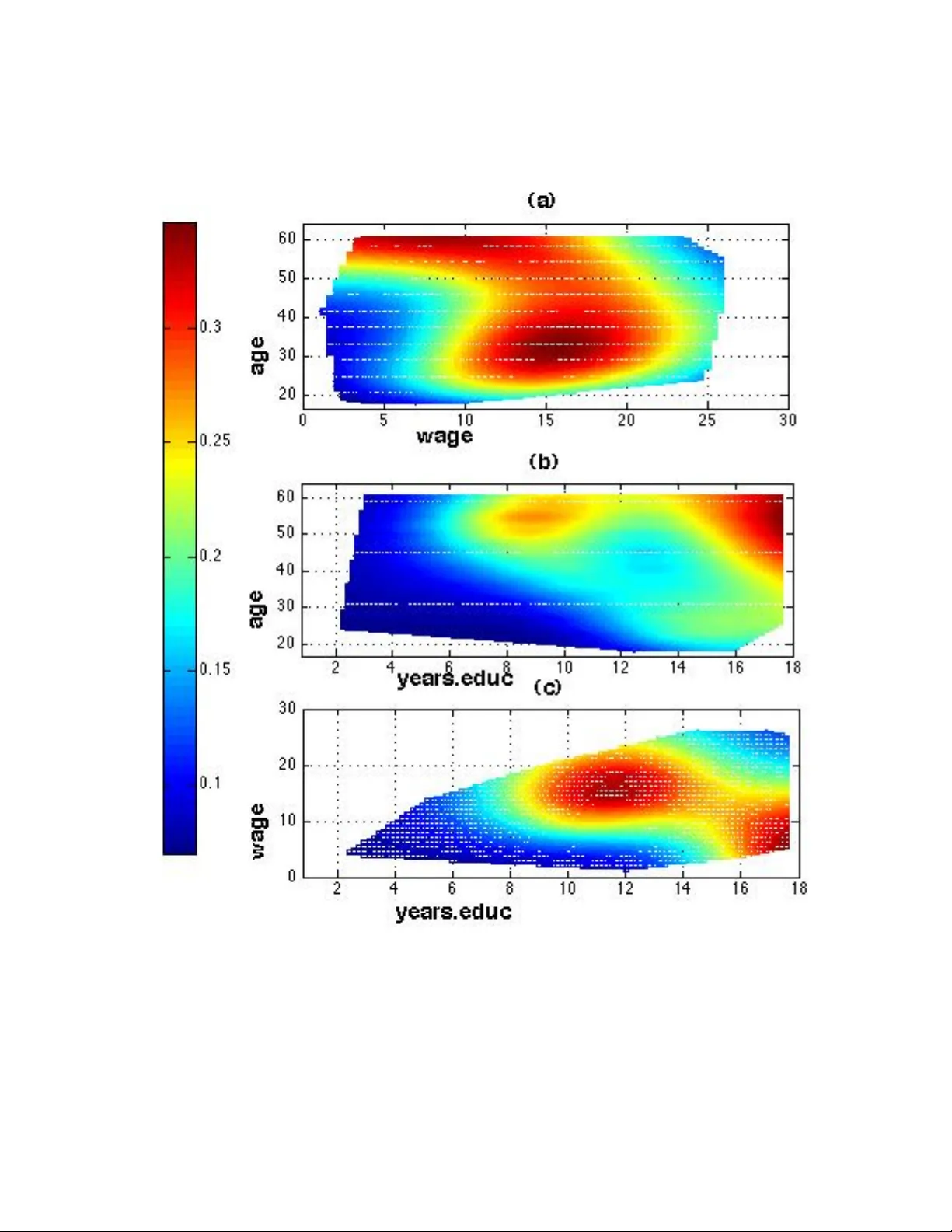
Lo cally Adaptiv e Nonparametric Binary Regression SALL Y A. W OOD, ROBER T K OHN and REMY COTTET University of New South Wales, Sydney, NSW, 2052, A ustr alia WENXIN JIANG and MAR TIN T ANNER Northwestern University, Evanston, Il linois, 60208 U.S.A. June 20, 2021 Abstract A nonparametric and lo cally adaptiv e Bay esian estimator is prop osed for esti- mating a binary regression. Flexibilit y is obtained by modeling the binary regres- sion as a mixture of probit regressions with the argumen t of eac h probit regression ha ving a thin plate spline prior with its own smo othing parameter and with the mixture w eigh ts dep ending on the cov ariates. The estimator is compared to a sin- gle spline estimator and to a recently prop osed lo cally adaptiv e estimator. The metho dology is illustrated by applying it to b oth sim ulated and real examples. KEY WORDS : Bay esian analysis; Marko v c hain Mon te Carlo; Mixture-of-Experts; Mo del a veraging; Surface Estimation; Rev ersible jump; 1 In tro duction Supp ose w e wish to model the spatial distribution of the habitat of the crested lark. One w ay to do this is to model the probability of a crested lark sigh ting as a function of latitude ( lat ) and longitude ( l on ) as Pr(crested lark sighting | lat, lon ) = H { g ( lat, l on ) } , (1.1) 1 where H is a link function, suc h as a probit or logit, and g is a function of latitude and longitude, whic h is either parametric or nonparametric. Our article presen ts a Ba y esian metho d for estimating the probability in (1.1) that do es not assume a parametric form for H and allows the probabilit y to b e lo cally adaptive with respect to the co v ariates, that is, to b e smooth in one region of the co v ariate space and wiggly or ev en discontin uous in another. W e mo del the binary regression as a mixture of probit binary regressions Pr(crested lark sighting | Lat, Lon ) = r X j =1 π j ( Lat, Lon )Φ { g j ( Lat, Lon ) } , (1.2) where Φ is the standard normal cumulativ e distribution function and the g j are truncated spline functions. W e demonstrate that the resulting estimators are nonparametric and lo cally adaptiv e, but do not o verfit. The reasons for this go od performance are that mixing is done outside the probit cum ulative distribution function rather than inside, the weigh ts π j are allo wed to v ary with the co v ariates, and that the comp onen t functions g j can hav e different lev el of smo othness by having different smo othing parameters. This is esp ecially important when mo deling surfaces in t w o or more dimensions where a single smo othing parameter for a m ultidimensional surface will often be inadequate. The use of truncated spline bases allo ws mo dels with sev eral thousand observ ations and regression surfaces with a mo derate num b er (at least 6 or 7) of cov ariates (provided the num b er of observ ations is adequate). Extending the methodology to higher dimensions problems is important b ecause as the n umber of co v ariates increase so to o do es the need for lo cal smo othing. This is b ecause the smo othness of the function H ( x ) is lik ely to b e different for different cov ariates. Our article allows the n umber of comp onen ts to v ary from r = 1 , . . . , R , with R typically 3 or 4. W e use a Bay esian approac h and construct a Marko v c hain Monte Carlo sampling scheme (MCMC) to estimate the mo del that uses the reversible jump method of Green (1995) to mo ve b etw een model spaces having different num b ers of comp onents. Mo del (1.2) is known as a Mixture-of-Exp erts (ME) mo del and was first in tro duced by Jacobs et al. (1991) and Jordan and Jacobs (1994), who used simple linear functions for the g j and estimated the mo del by the EM algorithm. 2 There is an extensiv e literature on estimating binary regressions. McCullagh and Nelder (1989) discuss parametric approaches. Nonparametric binary regression is discussed by W ang (1994, 1997), W ah ba, W ang, Gu, Klein and Klein (1997) and Loader (1999). W o od and Kohn (1998) and Holmes and Mallick (2003) presen t Bay esian approaches to nonparametric binary re- gression. Ho wev er, none of these pap ers show that their estimates are lo cally adaptive. Krib o v oko v a et al. (2006) present an estimator of a binary regression that is based on quasi lik eliho o d and sho w that it is lo cally adaptive. A n um b er of lo cally adaptiv e estimators ha v e recen tly b een prop osed for Gaussian re- gression mo dels. Most of these estimators represen t the unknown regression function as a linear com bination of basis functions. F requen tist approaches such as F riedman and Silver- man (1989), F riedman (1991) and Luo and W ahba (1997) sough t an optimal com bination of basis functions using a greedy search algorithm, whereas Bay esian approaches such as Smith and Kohn (1996) and Denison, Mallick and Smith (1998) av eraged o ver a large num b er of com binations of subsets of the basis functions. W o od, Jiang and T anner (2002) prop osed a lo cally adaptive estimator for Gaussian re- gression by mixing o ver a com bination of splines and used BIC to c ho ose the n umber of comp onen ts. Our article builds on this Mixture of Exp erts approach by W o od,et al. (2002). A direct w ay to obtain a locally adaptive estimator of binary probabilities is to adaptiv ely estimate g in (1.1) by using laten t v ariables together with the basis selection metho ds in F riedman (1991), Denison, Mallick and Smith (1998), and Smith and Kohn (1996) or with the mixture of splines metho d in W o o d et al. (2002). Ho wev er, we ha ve found that for the mixture of splines approach, adaptively estimating the regression function g by mixing on the inside of Φ results in p oor estimates of the probabilities due to o verfitting. Figure 1 gives an example of such ov erfitting. The figure shows the true probability H ( x ) = P r ( y = 1 | x ) and the estimate b H ( x ) = Φ( b g ( x )) where g ( x ) = π ( x ) f 1 ( x ) + (1 − π ( x )) f 2 ( x ), which we call mixing on the inside. The figure also sho ws the estimate of H ( x ) based on mo deling H ( x ) as π ( x )Φ { f 1 ( x ) } + (1 − π ( x ))Φ { f 2 ( x ) } , which w e call mixing on the outside. In this example, whic h is typical of all suc h examples, it is clear that mixing on the inside do es not p erform 3 as w ell as mixing on the outside. The tec hnical rep ort b y W o od, Kohn, Jiang and T anner (2005) pro vides details of why mixing on the inside tends to result in o verfitting and pro duces inferior estimates to mixing on the outside. 2 Mo del and Prior Sp ecification W e present the mo del in this section. Appendix A giv es details of the sampling scheme used to estimate the mo del. Using the results in Tierney (1994) and Green (1995) w e can sho w that the sampling scheme con verges to the p osterior distribution. Let w b e a binary response v ariable taking the v alues 0 and 1. W e mo del the binary regression of w on x b y a mixture of finite but unknown num b er of probit regressions, as Pr( w = 1 | x ) = R X r =1 H r ( x ) Pr( r ) , H r ( x ) = r X j =1 π j r ( x )Φ { g j r ( x ) } (2.1) with π j r ( x ) = exp( δ 0 j r z ) / r X k =1 exp( δ 0 kr z ) , j = 1 , . . . , r , where z = (1 , x 0 ) 0 . W e usually take the num b er of comp onen ts R as 3 or 4 with Pr( r ) = 1 /R , for r = 1 , . . . , R . Without loss of generalit y w e assume that the v ector δ 1 r = 0 and let δ r = ( δ 2 r , . . . , δ rr ) b e a vector of unconstrained co efficients. W e observe w 1 , . . . , w n as well as the corresp onding cov ariates x 1 , . . . , x n . T o place a prior on g j r w e write g j r ( x ) = α 0 j r z + f j r ( x ) (2.2) where α j r is a co efficient vector and f j r ( x ) is the nonlinear part of g j r . F or j = 1 , . . . , r , let f j r =  f j r ( x 1 ) , . . . , f j r ( x n )  0 . W e write f j r as a linear com bination of basis functions as outlined b elo w so that f j r = X β j r , where the columns of the design matrix X are partial thin plate spline basis functions and β j r is a v ector of co efficien ts. Appendix B describ es ho w we construct the design matrix X to handle a large num b er of observ ations n and a mo derate n umber of co v ariates. 4 The prior for α j r for j = 1 , . . . , r is N (0 , c α I ), for some large c α , and w e assume that the g j r ’s are indep endent apriori . Based on emprical evidence w e found that the regression function estimates w ere insensitiv e to the c hoice of c α o ver the range [10 2 , 10 10 ]. The prior for β j r ∼ N (0 , τ j r I ) , j = 1 , . . . , r . W e assume a uniform prior for τ 1 r ∼ U (0 , c τ ), for some large c τ . T o ensure iden tifiability we assume apriori that τ j r ∼ U (0 , τ ( j − 1) r ) for j = 2 , . . . , r , i.e., τ 1 r <, . . . , < τ rr < c τ . The prior on the parameter vector δ r for the mixing probabilities is N (0 , c δ I )), where c δ = n . 3 Sim ulations 3.1 Comparison with a single comp onent estimator The p erformance of the prop osed metho d is studied for four functions listed in table 1, using a sample size of n = 1000 for each function. The three univ ariate functions are plotted in Figure 3. The biv ariate function is plotted in Figure 4(a). The four functions are c hosen in suc h a wa y that each requires a different t yp e of smo othing. F unction (a) requires only one smo othing parameter, function (b) requires lo cal smoothing, function (c) is a discontin uous function, and function (d) is a discontin uous biv ariate function. The estimates obtained F unction Lab el F unction F ormula a (sin) Pr( w = 1 | x ) = Φ { 2 sin(4 π x ) } b (p eak) Pr( w = 1 | x ) = Φ { 5 6 exp h ( x − 0 . 1) 2 0 . 18 i + 1 3 exp h ( x − 0 . 6) 2 0 . 004 i − 1 } c (step) Pr( w = 1 | x ) = Φ {− 1 . 036 + 2 . 073 I x (0 . 25) − 1 . 42712 I x (0 . 75) } where I x ( a ) = 1 if x > a d (cylinder) Pr( w = 1 | x ) = D { ( x − 0 . 5) 2 + ( y − 0 . 5) 2 − 0 . 16 2 } where D ( x ) = 0 . 8 if x < 0 and D ( x ) = 0 . 2 if x > 0 T able 1: Regression functions used in sim ulations using the prop osed method are compared to estimates obtained using a single component 5 estimator as in W o od and Kohn (1998). W e use this estimator for comparison b ecause W o od and Kohn (1998) sho w that their single spline estimator outp erforms other av ailable estimators, suc h as GRKP ACK by W ang (1997). Fift y replications w ere generated for eac h regression function using a maximum R = 3 comp onen ts. W e use the a verage symmetric Kullbac k-Leibler distance to measure performance. This measure is also used by Gu (1992) and W ang (1994), and is defined b elo w. Let I { H ( x i ) , b H ( x i ) } = c Pr( w i = 0 | x i ) log ( c Pr( w i = 0 | x i ) P r ( w i = 0 | x i ) ) + c Pr( w i = 1 | x i ) log ( c Pr( w i = 1 | x i ) Pr( w i = 1 | x i ) ) . By Rao (1973, pp. 58-59), I { H ( x i ) , ˆ H ( x i ) } ≤ 0 and I { H ( x i ) , b H ( x i ) } = 0 if and only if H ( x i ) = b H ( x i ) at the design p oin ts. The av erage symmetric Kullbac k-Leibler distance (ASKLD) b et ween H and b H is defined as AS K LD ( H , b H ) = 1 n n X i =1 h I { H ( x i ) , b H ( x i ) } + I { b H ( x i ) , H ( x i ) } i . It follows from the prop erties of the Kullbac k-Leibler distance that AS K LD ( H , b H ) ≤ 0 and AS K LD ( H , ˆ H ) = 0 if and only if b H = H . Th us, the closer I ( H , b H ) is to zero the b etter. F or each replication, the ASKLD was calculated for b oth estimators, where b H ( x i ) is the estimate obtained for the function P r ( w i = 1 | x i ). Figure 2 compares the p erformance of the mixture estimator with the p erformance of the single comp onen t estimator using b o xplots, with each b o xplot represen ting the av erage difference in ASKLD for the fifty replications for that function. A p ositiv e difference means that the mixture mo del p erforms b etter than the single spline estimator for that replication, while a p ositive difference means the opp osite. Figure 2 sho ws that the mixture of splines estimator performs significan tly b etter in terms of the ASKLD than the single spline estimator when the regression surface is heterogenous, that is when it requires lo cal smo othing. In particular, for the heterogeneous functions (b), (c) and (d) the mixture estimator outp erformed the single spline. F urthermore, when the function is homogenous, that is when it do es not require lo cal smo othing, the mixture estimator p erforms almost as well as a single spline estimator b ecause when only one spline is needed, for example for function (a), the p osterior probability of a single spline is high. 6 T able 2 giv es the a verage (o ver the 50 replications) p osterior probability of the num b er of splines needed for mixing for each of the four regression functions. The table shows that for the homogenous function (a) the a verage p osterior probabilit y that only one spline is need is 0.78. In general we ha ve found that for homogenous functions the p osterior probability of a single comp onen t is high. Conv ersely , we hav e found that for heterogenous functions the pos- terior probability of requiring more than a single comp onen t is high. Thus, for function (b), the a verage p osterior probabilit y is 0.76 that t wo splines are needed and 0.24 that three spline are needed. F or the piecewise constan t functions (c) and (d), the a verage p osterior probabilities that t wo splines are needed are 0.60 and 0.84 resp ectiv ely , whereas the av erage p osterior probabilities that three splines are need is 0.37 and 0.08 resp ectiv ely . F unction Lab el Pr( r | w ) 1 2 3 a (sin) 0 . 78 0 . 21 0 . 01 b (p eak) 0 . 00 0 . 76 0 . 24 c (step) 0 . 03 0 . 60 0 . 37 d (cylinder) 0 . 08 0 . 84 0 . 08 T able 2: Average p osterior probabilit y of n umber of splines needed T o see ho w the difference in ASKLD translates into differences in the regression function estimates, the estimates for functions (a)-(c) corresp onding to the 10th p ercen tile, 50th p er- cen tile and 90th p ercen tile ASKLD are plotted in Figure 3. Figure 3 shows that an estimator based on a mixture of splines can accurately estimate b oth homogeneous and heterogeneous functions. When the function is homogeneous, e.g. function (a), the mixture estimates are visually indistinguishable from the single spline estimates. Ho wev er, when the function is heterogeneous, the single spline estimates are muc h worse than the mixture estimates. F or example, ev en the 90 th p ercen tile of the single spline estimate of function (b) fails to cap- ture the p eak on the left and ov erfits on the right, whereas the mixture estimate do es w ell throughout the whole range of the function. Figure 4 plots the fit for the cylinder data for a single spline and a mixture of splines. The improv ement is mark ed, with the single spline 7 b eing unable to capture the sudden change of curv ature. 3.2 Comparison to a lo cally adaptive estimator Krib o v oko v a et al. (2006) prop ose a general approac h for lo cally adaptive smo othing in regression mo dels with the regression function mo deled as a p enalized spline that has a smo othly v arying smo othing parameter function whic h is also mo deled as a p enalized spline. In particular, their approach handles lo cal smo othing of binary data. The authors hav e implemen ted their approach in a pac k age called Adaptfit which is written in R and is av ailable at http://cran.r-pro ject.org/src/con trib/Descriptions/AdaptFit.html. This section compares our approach to that of Krib o vok o v a et al. (2006) as implemented in Adaptfit in terms av erage squared error, co v erage probabilities and running time for the four functions (a)–(d). The results rep orted b elo w are each based on 50 replications unless stated otherwise. Let ASE M E b e the av erage s quared error ov er the ab cissae of the data of the Bay esian ME estimator and let ASE AF b e the corresp onding av eraged squared error of the Adaptfit estimator. W e define the p ercentage change in going from the ME estimator to the adaptfit estimator as %∆ASE = AS E AF − AS E M E AS E M E × 100 . T able 3 rep orts the 25th, 50th, 75th p ercen tiles and the mean of %∆ASE and shows that the ME estimator and the Adaptfit estimator perform similarly for functions (a) and (b), but that the ME of exp erts estimator outp erforms the Adaptfit estimator for functions (c) and (d). Let the empirical co verage probability ECP M E ( x ) b e the prop ortion (out of 50) of 90% p oin t wise confidence interv als that con tain the true probabilit y at the ab cissa x for the ME estimator. Let ECP AF ( x ) be defined similarly for the Adaptfit estimator. Figure 5 plots ECP M E ( x i ) and ECP AF ( x i ) at the ab cissae x i of the data for the functions (a)–(c). Figure 6 8 is a similar plot for the cylinder function (d). Let %∆AECP M E = 100 ×  n − 1 n X i =1 ECP M E ( x i ) − 0 . 9  / 0 . 9 b e the p ercen tage deviation from 0.9 of the av erage of the ECP M E ( x i ) o ver all the x i ab cissae of the data. Let %∆AECP AF b e defined similarly for the Adaptfit estimator. T able 3 rep orts b oth %∆AECP M E and %∆AECP AF . Figure 5 and table 3 suggest that the empirical co verage probabilities of the ME estimator and Adaptfit are similar for functions (a) and (b), while the ME estimator has sup erior empirical co verage probabilities for functions (c) and (d). F unction %∆ASE %∆AECP 25 50 75 mean ME AF (a) Sin − 11 . 32 7 . 86 29 . 64 11 . 18 − 0 . 74 3 . 10 (b) Peaks − 8 . 03 − 0 . 703 15 . 07 7 . 72 − 3 . 34 − 5 . 89 (c) Step 52 . 23 93 . 15 140 . 23 101 . 99 − 9 . 07 − 18 . 12 (d) Cylinder 86 . 28 130 . 76 162 . 11 126 . 83 − 16 . 80 − 26 . 62 T able 3: Comparison of Ba yesian ME and adaptfit. The first four columns giv e the 25th, 50th , 75th p ercen tiles and the mean of the p ercen tage difference b et ween the a veraged mean squared error of adaptfit and the ME estimators. The next tw o columns giv es the p ercen tage co verage errors of the 90% confidence interv als for ME and Adaptfit. W e now discuss some computational issues that determine the p erformance of Adaptfit in the binary regression case. Adaptfit uses tw o sets of knots. The first set of knots is for the p enalized spline basis for the regression function and the second set of knots is for the p enalized spline basis for the smoothing parameters. See Kribov oko v a et al. (2006) for details. Let K b b e the num b er of knots chosen for the first p enalized spline and K c the num b er of knots chosen for the second penalized spline. W e found in the binary case that if a function requires a lo cally adaptiv e estimator then to get a satisfactory fit it may be necessary to tak e K b quite large. F or example, for the p eak function (b) and the cylinder function (d) it seems necessary to tak e K b = 120 to 150. The results for functions (a), (c) and (d) in table 3 9 w ere obtained using using K b = 150 and K c = 20. The results for function (b) (peak) were supplied to us by Dr T at yana Kriv ob ok ov a who used an Splus implemen tation of Adaptfit b ecause we were unsuccessful with the R implemen tation . The results rep orted for Adaptfit for function (b) are for 47 replicates with the other three replicates b eing unsatisfactory . Adaptfit also has a default c hoice of K b and K c and we chec ked that the ab o ve settings for functions (a), (c) and (d) gav e as go o d or b etter p erformance as the defaults. The times giv en b elo w are a verages ov er sev eral replications and were obtained on a 2.8GHz PC running Matlab 7. F or function (a), Adaptfit took 25 seconds for the default n umber of knots and 320 seconds for ( K b , K c ) = (150 , 20). F or function (c), Adaptfit to ok 36 seconds for the default num b er of knots and 325 seconds for ( K b , K c ) = (150 , 20). F or function (d), Adaptfit did not giv e satisfactory results for the default n um b er of knots and to ok 316 seconds for ( K b , K c ) = (150 , 20). The ME estimator takes ab out 90 seconds p er 2000 iterations for eac h of the examples in this section. F or each of the examples rep orted in this section and the next section w e ran the ME estimator for 10000 iterations in total (5000 warm up and 5000 sampling), that is, the time taken for each of the examples in this section is ab out 450 seconds. How ever, w e ha ve found in extensive testing that it is sufficien t to use 4000 to 6000 iterations in all of these examples, that is about 180 to 270 seconds in total. All the times rep orted were recorded on a 2.8GHz PC running Matlab 7. Thus Adaptfit can b e v ery fast when the default n umber of knots is used, but for a binary regression it is difficult to determine apriori for any data set whether the default n umber of knots is adequate and in our opinion it is safer to take the more conserv ative approac h b y setting K b to 120 or 150. In that case the times required by Adaptfit and the ME estimators are not that differen t, while the ME estimator in the binary case app ears computationally more robust. 10 4 Real Examples 4.1 Probabilit y of crested lark sigh ting in Portugal This section demonstrates how the prop osed metho d can b e used to mo del spatial data b y mo delling the probabilit y of a crested lark sightin g at v arious lo cations in P ortugual. The data w ere obtained from W o od (2006). Eac h observ ation refers to one tetrad (2km by 2km square) and contains a v ariable indicating whether the crested lark was sighted in the tetrad or not together with the lo cation of the tetrad. The location of a tetrad is identified by kilometers east and north of an origin. Portugal can b e divided into 25100 tetrads for which there w ere observ ations on 6457 tetrads. This dataset was analysed by W o od (2006) who aggregated the data into 10km b y 10km squares and fitted a binomial generalized additive mo del (GAM) using thin plate regression splines to the aggregated resp onse. In their example the degree of smo othness w as estimated using the un-biased risk estimator (UBRE), which w as then scaled- up b y a factor of 1.4 to av oid ov erfitting. The factor b y which the smoothing parameter is rescaled is chosen sub jectiv ely and affects the estimated probabilities substantially . In con trast, our metho d allows for the degree of smo othness to v ary across the cov ariate space and the estimated probabilities are therefore spatially adaptive . Our mo del for the probability of a crested lark sigh ting is given by (2.1) and (2.2) with x = ( east, nor th ), where east and nor th mean kilometers east and north of an origin. The dep enden t v ariable is 1 if a crested lark is sigh ted in a tetrad and 0 if it is not. W e assume a maximum of four mixture comp onen ts. W e considered the choice of the num b er of mixture comp onen ts in several wa ys. First, the p osterior probabilities for 1 to 4 components are 0.0, 0.94, 0.04 and 0.01, suggesting a t wo comp onen t mixture. W e also lo oked at the empirical receiv er op erating curv es (ROC) for mo dels with 1 to 4 comp onen ts. See F an, Upadhy e and W orster (2006) for a description of ROC curves. In our case a ROC curve sho ws the trade off b et ween classifying a tetrad as con taining the crested lark when the tetrad do es contain the crested lark versus classifying a tetrad as containing the crested lark when it do es not. The larger the area under the 11 R OC curve the more effective is the mo del at classifying. Out of 6457 observ ations we randomly selected 5817 for mo del fitting and set aside 640 for mo del testing. W e estimated the probability that a tetrad contains the crested lark using mixture mo dels containing one to four components. F or each mixture mo del w e then used the estimated probabilities to classify the 640 observ ations set aside for mo del testing. Figure 7 plots the empirical R OC curv es based on these 640 observ ations and shows the improv ement in classification that is ac hieved b y using a mixture of tw o splines ov er a single spline. Figure 7 also shows that there is not muc h improv ement in classification in mo ving from a mixture of tw o to a mixture of three or four and hence supports the choice of a mixture of tw o splines as the preferred mo del. This finding is consistent with the p osterior probabilities of the num b er of comp onents. Figure 8 shows con tour plots for the probabilit y of a crested lark sighting for a single spline estimator and a mixture of s plines estimators. This figure and the land use and p opulation maps, repro duced in figure, 9 sho w wh y a mixture of at least 2 splines is necessary . Mainland Portugal is split by the river T agus. The p opulation and land use maps show that the p opulation of P ortugal is concentrated to the north of the river, in particular in the north west where the land is giv en ov er to wine pro duction. The interior of the north is dry and mountainous. T o the south of the riv er the predominan t land form is rolling hills and the area is muc h less densely p opulated. The cultiv ated areas in the south are primarly for cork pro duction but there are large tracts of forested areas. Figure 8(b) shows that in the southern part of Portugal the probabilit y of sighting a crested lark v aries considerably and that these v ariations can o ccur abruptly . These abrupt c hanges corresp ond to c hanges in the top ography of southern P ortugal. The areas of high probabilit y corresp ond to forested/tree crop areas or ma jor rivers. The areas of low proba- bilit y corresp ond to pasturable lands. In contrast the probabilit y of a crested lark sighting in the northern part of Portugal has little v ariation; the high p opulation density together with the mountainous in terior means that the probabilit y is of sighting is uniformly low. Th us the degree of smoothing required dep ends on the co v ariates east and nor th . Figure 8 (a) sho ws that a single spline estimator cannot simultaneously capture the abrupt changes in southern 12 P ortugal and the smo oth changes in the north. 4.2 Probabilit y of b elonging to a union This example shows how our metho dology can b e extended higher dimensions by mo deling the probabilit y of union membership as a function of three con tinuous v ariables, ye ars e duc ation , wage and age , and three dummy v ariables, south (1=live in southern region of USA), female (1=female) and marrie d (1=married). The data consists of 534 observ ations on US work ers and can b e found in Berndt (1991) and at http://lib.stat.cm u.edu/datasets/CPS 85 W ages. Rupp ert, W and and Carroll (2003) estimate the probability of union membership using a generalized additive mo del without interactions. W e mo del the three dimensional surface of the con tinuous cov ariates and our results suggest that this more appropriate than an additiv e mo del. Our mo del for the probability of union membership is given by (2.1) with x =( ye ars e duc ation, wage, age, south, female, marrie d ). Ho wev er, w e mo dify the regression function (2.2) to take in to accoun t that three of the co v ariates are dumm y v ariables and should be excluded from the non-parametric component b y writing g j r ( x ) = α 0 j r z + f j r ( x ∗ ) where x ∗ = ( ye ars e duc ation , wage , age ), wage is in US $/hr and age is in y ears. The dep enden t v ariable is 1 if the work er b elongs to a union and 0 otherwise. Our metho d c ho oses one component 100% of the time. Figures 10 (a) - (c) show the join t marginal effect of t wo cov ariates at the mean of the third one and setting the dumm y v ariables to zero. These figures clearly s ho w interactions among the contin uous cov ariates. F or example figure 10 (a) shows that for work ers whose age is less than 40, the probabilit y of union membership initially increases with w age , b efore reac hing a p eak at a wage of ab out $15 /hr and then declines. F or older work ers this p eak o ccurs at muc h low er wages, somewhere b et w een $5/hr and $10/hr b efore declining sharply . Figure 10 (b) sho ws t wo mo des. F or w orkers with an a verage wage , union mem b ership peaks at 55 years and 8-10 ye ars e duc ation . In terestingly union mem b ership p eaks again at 55 y ears and 18 ye ars e duc ation , although 13 this p eak ma y b e due to b oundary effects. Figure 10 (c) sho ws that for w orkers who did not finish high school ( < 12 ye ars e duc ation ) the probabilit y of b elonging to union increases as wage increases. In contrast, for work ers with some tertiary education( > 14 ye ars e duc ation ) the probabilit y of b elonging to a union is initially high and then decreases with increasing wage . Ac kno wledgmen t W e thank the referee, the asso ciate editor and the editor for suggestions that improv ed the con tent and qualit y of the pap er. W e would especially like to thank Dr T at yana Kriv ob ok ov a for helping with the Adaptfit pac k age and for carrying some of the computations for us. Sally W o od, Rob ert Kohn and Rem y Cottet were supp orted by an AR C grant. App endix A: Sampling sc heme W e estimate the binary regression probabilities b y their p osterior means, with all unkno wn parameters and latent v ariables in tegrated out. T o mak e it easier to sim ulate from the p osterior distribution we introduce a n umber of latent v ariables that are generated during the simulation and turn (2.1) into a hierarch ical model. The first is the num b er of comp onen ts r at any p oin t in the simulation. Giv en r , define the v ector of multinomial random v ariables γ r = { γ r ( x 1 ) , . . . , γ r ( x n ) } such that γ r ( x i ) identifies the comp onen t in the mixture that w i b elongs to. W e assume that Pr( γ r | r , δ r , x ) = n Y i =1 Pr { γ r ( x i ) | r , δ r , x } , with Pr { γ r ( x i ) = j | δ r } = π j r ( x i ) and Pr( w | r , γ r , g r ) = n Y i =1 Pr { w i | γ r ( x i ) = j, g j r ( x i ) } T o estimate the comp onen t splines, we follo w Alb ert and Chib (1993) and W o od and Kohn (1998) and introduce a second level of latent v ariables, v ij r , also conditional on r , suc h 14 that v ij r = z i α j r + f j r ( x i ) +  ij r for j = 1 , . . . , r and i = 1 , . . . , n, where  ij r ∼ N (0 , 1). The laten t v ariable v j ir and the indicator v ariable γ r ( x i ) are related to eac h other and the observ ation w i b y requiring that v ij r > 0 if w i = 1 and γ r ( x i ) = j v ij r < 0 if w i = 0 and γ r ( x i ) = j. If γ r ( x i ) 6 = j , then v ij r is unconstrained. The sampling sc heme mo v es betw een models with differing n umbers of comp onen ts b y using rev ersible jump MCMC. T o implement a reversible jump step to go from a mo del with r components to a model with r 0 comp onen ts it is necessary to hav e a prop osal densit y in the r 0 comp onen t space. W e form such prop osals b y first running separate MCMC samplers for each r = 1 , . . . , R comp onen t mo dels. This sampling sc heme is describ ed b elo w under the heading of ‘Up dating within a mo del.’ W e now describ e the complete sampling scheme. First, r is initialized b y drawing it from the prior Pr( r = j ) = 1 /R, j = 1 , . . . , r . Conditional on this v alue of r , we initialize β r , α r , τ r , δ r b y the p osterior means of the iterates of the mo del with r comp onen ts. 1. Mo ving Betw een Mo dels Let X c = ( r c , Θ c r ) be the curren t v alue of the parameters in the c hain, where Θ c r = ( α c r , β c r , δ c r ). W e propose a new v alue of X p = ( r p , Θ p r ) and accept this prop osal using a Metropolis-Hastings (M-H) step. The M-H probability of accepting suc h a prop osal is  ( X c , X p ) = min  1 , p ( X p | w ) q ( X p , X c ) p ( X c | w ) q ( X c , X p )  = min  1 , p ( w | X p ) p ( X p ) q ( X p , X c ) p ( w | X c ) p ( X c ) q ( X c , X p )  , (A.1) where q ( X c , X p ) is an arbitrary transition probabilit y function that mo v es the c hain from X c to X p . 15 The prop osal density q ( X c , X p ) is given by q ( r c → r p ) q (Θ c r c → Θ p r p | r p ). That is, a new v alue r p of r is prop osed and Θ p r is prop osed conditional r p . The v alue of r p is prop osed as follows: (a) If 1 < r c < R then q ( r c → r p = r c ± 1) = 0 . 5 (b) If r c = 1 then q ( r c → r p = 2) = 1 (c) If r c = R then q ( r c → r p = R − 1) = 1 Then, conditional on r p , we prop ose new v alues of the parameter Θ p r p = ( δ p r p , β p r p , α p r p ) b y doing the follo wing. T o simplify notation, w e write r p as r . (a) Dra w δ p r from M V T 5 ( ˆ δ , ˆ Σ δ r ), where ˆ δ r and ˆ Σ δ r are the sample mean and co- v ariance of the iterates δ [ k ] r from the individual MCMC scheme for a mixture of r comp onen ts. W e use the notation M V T 5 ( a, B ) to denote a m ultiv ariate t distribution with 5 degrees of freedom, lo cation v ector a and scale matrix B . (b) Dra w β ∗ p r = ( β p r , α p r ) from M V T 5 ( ˆ β ∗ r , ˆ Σ β ∗ r ). where ˆ β ∗ r and ˆ Σ β ∗ r are the sample mean and co v ariance of the iterates β ∗ [ k ] r from the individual MCMC sc heme for a mixture of r comp onents. The sampling sc heme for a mo del of an r comp onen t mixture is identical to the sc heme for a within mo del mov e (step 2 b elo w). 2. Updating within Mo del Giv en the new v alues of r , δ r , and g r , the parameters sp ecific to that mo del are up dated as follows: (a) Dra w γ r , V r sim ultaneously from P ( γ , V r | w , g r , δ r , τ r ) by first drawing γ r and then drawing V r conditional on the v alue of γ r . i. T o draw γ r from Pr( γ r | w , δ r , g r ) note that Pr( γ r | w , δ r , g r ) = n Y i =1 Pr { γ r ( x i ) | w i , δ r , g j r ( x i ) } . 16 If w i = 1 then, Pr { γ r ( x i ) = j | w i = 1 , δ r , g r } = Pr { w i = 1 | γ r ( x i ) = j, δ r , g j r ( x i ) } Pr { γ r ( x i ) = j | δ r } P r k =1 Pr { w i = 1 | γ r ( x i ) = k , g kr ( x i ) , δ k } Pr { γ r ( x i ) = k | δ r } = Φ { g j r ( x i ) } Pr { γ r ( x i ) = j | δ r } P r k =1 Φ { g k ( x i ) } Pr { γ r ( x i ) = k | δ r } . Similarly , if w i = 0 then, Pr { γ r ( x i ) = j | w i = 0 , δ r , g r } = [1 − Φ { g j r ( x i ) } ] Pr { γ r ( x i ) = j | δ r } P r k =1 [1 − Φ { g kr ( x i ) } ] Pr { γ r ( x i ) = k | δ r } . ii. T o draw V r from p ( V r | w , γ r , g r ) note that, p ( V r | , w , γ r , g r ) = n Y i =1 r Y j =1 p ( v ij r | g j r ( x i ) , γ r ( x i ) , w i ) . If γ r ( x i ) = j and w i = 1, then v ij r ∼ N ( g j r ( x i ) , 1), and is constrained to b e p ositiv e. If γ r ( x i ) = j and w i = 0, then v ij r ∼ N ( g j r ( x i ) , 1), and is constrained to b e negativ e. If γ r ( x i ) 6 = j then dra w v ij r from its unconstrained distribution, whic h is N ( g j r ( x i ) , 1). (b) Dra w δ r from p ( δ r | γ r ) using a M-H step. The conditional p osterior distribution of δ r is p ( δ r | w , γ r ) = p ( δ r | γ r ) ∝ p ( γ r | δ r ) p ( δ r ) = p ( δ r ) n Y i =1 exp { P r j =1 δ j r z i γ r ( x i ) } P r k =1 exp { δ kr z i } (A.2) and δ r ∼ N (0 , 10 I ). Our prop osal densit y is M V T 5 ( δ max , V δ ) where δ max is that v alue of δ r that maximizes p ( δ r | w , γ r ) in (A.2), and V δ is the negative of the in verse of the second deriv ative of log [ p ( δ r | w , γ r )]. (c) Dra w β r , α r sim ultaneously from p ( β r , α r | V r , τ r ) by first dra wing α r and then conditional on this v alue of α r dra wing β r : 17 i. T o draw α r note that p ( α r | V r , τ r ) = r Y j =1 p ( α j r | v j , τ j r ) and p ( α j r | v j , τ j r ) ∼ N ( M α , V α ) where, V α = [ Z 0 Z − Z 0 X τ j r [ τ j r X 0 X + I ] − 1 X 0 Z ] − 1 and M α = V α  Z 0 v j r − Z 0 X τ j r [ τ j r X 0 X + I ] − 1 X 0 v j r  . ii. T o draw β r note that p ( β r | V r , τ r , α r ) = r Y j =1 p ( β j r | α j r , v j r , τ j ) and p ( β j r | v j r , τ j r , α j r ) ∼ N ( M β , V β ) where V β = τ j r [ τ j r X 0 X + I ] − 1 whic h is diagonal and M β = V β X 0 v j r and v j r = v j r − Z α j r . (d) Dra w τ r sim ultaneously from p ( τ r | β r ) by drawing from p ( τ r | β r ) = r Y j =1 p ( τ j r | β j r ) and then re-label γ r ( x i ) for i = 1 , . . . , n so that τ 1 r , > . . . , > τ rr (see Stephens, 2000). App endix B: Constructing the design matrix This app endix outlines how we construct the design matrix X to allo w for a large n umber of observ ations and a mo derate num b er of co v ariates. 18 1. Normalize the v alues of all co v ariates to lie in the interv al [0,1] 2. Choose the n um b er m and lo cation of knots, so that in a giv en h yp ercube of width  , (  is t ypically chosen to b e 0.05) and dimension p , a knot is placed at the cen tre of gravit y of the hypercub e. If there are no p oin ts in a h yp ercub e then a knot is not c hosen for that hypercub e. If the data are equally spaced across a grid where the grid length =  then this results in m = n . If the data are clustered, as is often the case in high dimensional data, then this tec hnique results in m < n . 3. Let ˜ x j b e the p osition of the j th knot and let x ∗ i b e the i th ro w of the normalized co v ariates. Radial basis functions, denoted by φ ij , are constructed such that φ ij = || x ∗ i − ˜ x j || a ∗ log ( || x ∗ i − ˜ x j || ) , a = 2 ∗ ceil( p 2 + 0 . 1) − p , where ceil( x ) means to round x up to the nearest integer v alue. This means that the ( i, j ) th elemen t of the n × m design matrix X is equal to φ ij for i = 1 , . . . , n and j = 1 , . . . , m . 4. T o limit the dimension of the design matrix w e tak e a singular v alue decomp osition of X , s.t. X = U Λ V 0 where U and V 0 are square, orthonormal matrices and Λ is an n × m matrix, with nonnegative num b ers on the diagonals, λ ii for i = 1 , . . . , m where λ 11 > . . . > λ mm , and zeros off the diagonal. W e then let λ ii = 0 for i > l 0 , where l 0 = 25. W e choose l 0 in this wa y b ecause t ypically 1 − P l 0 i =1 λ 2 ii / P m i =1 λ 2 ii < 1 × 10 − 10 . 5. W e re-form X by letting X = U Λ. The design matrix X is no w a n × l 0 matrix. Note that X X 0 = U Λ 2 U 0 has the eigenv alue decomposition QD Q 0 , so that the resulting n × l 0 design matrix could hav e b een formed by performing an eigenv alue decomp osition on the n × n matrix X X 0 = QDQ 0 and setting d i = 0 for i > l 0 , how ever if n is large p erforming an eigen v alue decomp osition is computationally in tractable. References Alb ert, J. and Chib, S. (1993). Ba yesian analysis of binary and p olyc hotomous resp onse data. Journal of the Americ an Statistic al Asso ciation , 88 , 669–679. Berndt E. R., The practice of Econometrics, New Y ork: Addison-W esley . (1991) 19 Denison, D.G.T., Mallic k, B.K. & Smith, A.F.M. (1998). Automatic Bay esian curve fitting. Journal of the R oyal Statistic al So ciety B , 60 , 333–350. F an, J., Upadhy e, S. and W orster, A. (2006). Understanding receiv er op erating characteristic (R OC) curves, Canadian Journal of Emer gency Me dicine . 8 , 19-20. h ttp://www.caep.ca/template.asp?id=C4F7235436434ADAAB02D6B3E9C7A197 F riedman, J.H. and Silverman, B.W. (1989). Flexible parsimonious smo othing and additiv e mo deling, T e chnometrics . 31 , 3-39. F riedman, J.H. (1991). Multiv ariate adaptive regression splines (with discussion), The Annals of Statistics 19 , 1-141. Green, P .J. (1995) Reversible jump MCMC computation and Bay esian mo del determination. Biometrika , 82 , 711-732. Gu, C. (1992), Cross-v alidating non-Gaussian data, Journal of Computational and Gr aphic al Statistics , 1 , 169-179. Holmes, C.C. and Mallick, B.K. (2003) Generalized Nonlinear Mo deling With Multiv ariate F ree-Knot Regression Splines, Journal of the A meric an Statistic al Asso ciation, 98 , 352- 368. Jacobs, R.A., Jordan, M.I., Nowlan, S.J. and Hin ton, G.E. (1991). Adaptiv e mixtures of lo cal exp erts, Neur al Computation 3 , 79–87. Jordan, M.I. and Jacobs, R.A. (1994). Hierarchical mixtures-of-exp erts and the EM algo- rithm, Neur al Computation 6 , 181-214. Kriv ob ok ov a, T., Crainiceanu, C.M. and Kauermann, C. (2006) F ast adaptiv e penalized splines. T o app ear in Journal of Computational and Gr aphic al Statistics . Loader, C. (1999). L o c al r e gr ession and likeliho o d , New Y ork: Springer 20 Luo, Z. and W ahba, G. (1997). Hybrid adaptive splines, Journal of the Americ an Statistic al Asso ciation 92 , 107-114. McCullagh, P . and Nelder, J.A. (1989). Gener alize d line ar mo dels (2nd e dition) , New Y ork: Chap- man Hall. Rao, C.R. (1973, Line ar statistic al infer enc e and it applic ations (2nd e dition) , New Y ork: John Wiley . Rupp ert D., W and, M.P . and Carroll R.J. (2003). Semip ar ametric R e gr ession . Cam bridge Univ ersity Press. Smith, M. and Kohn, R. (1996). Nonparametric regression using Ba yesian v ariable selection, Journal of Ec onometrics 75 , 317-344. Stephens, M. (2000). Dealing with lab el-switc hing in mixture mo dels. Journal of the R oyal Statistic al So ciety B , 62 , 795–809. Tierney , L. (1994). Mark ov c hains for exploring p osterior distributions (with discussion). The A nnals of Statistics , 22 , 1701-1762. W ahba, G., W ang, Y., Gu, C., Klein, R. and Klein, B (1997). “Smo othing spline ANO V A for exp onen tial families, with application to the Wisconsin epidemiological study of diab etic retinopath y”, Annals of Statistics , 23 , 1865–1895. W ang, Y. (1994), Unpublished do ctoral thesis, Univ ersity of Wisconsin-Madison. W ang, Y. (1997). GRKP ACK: Fitting Smoothing Spline ANO V A Mo dels for Exp onen tial F amilies, Communic ations in Statistics: Simulation and Computation , 26 , 765–782. W o od, S.A. and Kohn, R. (1998). A Bay esian approach to robust binary non-parametric regression, Journal of the Americ an Statistic al Asso ciation, 93 , 203–213. W o od, S.A., Jiang W. and T anner, M.A. (2002). Ba yesian mixture of splines for spatially adaptiv e nonparametric regression, Biometrika , 89 , 513-528. 21 W o od, S.A., Kohn, R., Jiang W. and T anner, M.A. (2005). Mixing on the outside, Unpub- lishe d te chnic al R ep ort, University of New South Wales . W o od, S.N. (2006). Gener alize d A dditive Mo dels: An Intr o duction with R , Chapman Hall/CR C 0 0.1 0.2 0.3 0.4 0.5 0.6 0.7 0.8 0.9 1 0 0.1 0.2 0.3 0.4 0.5 0.6 0.7 0.8 0.9 1 Figure 1: The solid line gives the true function H ( x ) (T able 1 function (b)). The dotted line (...) is the estimate ˆ H ( x ) for mixing on the inside while the dashed line (- - -) is the estimate ˆ H ( x ) for mixing on the outside. 22 sin peak step cylinder ! 0.01 ! 0.005 0 0.005 0.01 0.015 0.02 0.025 0.03 0.035 0.04 Figure 2: Boxplots of the ASKLD b etw een an estimate based on a mixture of splines and an estimate based on a single spline for the functions in table 1. Note that if the ASKLD > 0 then the estimator based on a mixture of splines is better than the estimator based on a single spline. 23 0.4 0.9 x 0.0 0.2 0.4 0.6 0.8 1.0 (a) 0.4 0.9 x 0.0 0.2 0.4 0.6 0.8 1.0 (b) 0.4 0.9 x 0.0 0.2 0.4 0.6 0.8 1.0 (c) 0.4 0.9 x 0.0 0.2 0.4 0.6 0.8 1.0 (d) 0.4 0.9 x 0.0 0.2 0.4 0.6 0.8 1.0 (e) 0.4 0.9 x 0.0 0.2 0.4 0.6 0.8 1.0 (f) 0.4 0.9 x 0.0 0.2 0.4 0.6 0.8 1.0 (g) 0.4 0.9 x 0.0 0.2 0.4 0.6 0.8 1.0 (h) 0.4 0.9 x 0.0 0.2 0.4 0.6 0.8 1.0 (i) Figure 3: Panels (a)–(c) plot the estimates corresp onding to the 10th worst p ercen tile ASKLD for functions (a) - (c) in table 1. Panels (d)–(f ) and panels (g)–(i) are similar plots corre- sp onding to the 50th p ercen tile ASKLD and 10th b est p ercen tile ASKLD, resp ectiv ely . In all cases n = 1000 and the true function H ( x ) is given by the dotted line, the estimate based on a mixture is given by the thic k solid line and the estimate based on a single spline is given b y the thin solid line. 24 Figure 4: Cylinder data, panel (a) plots the true function and data, panel (b) plots the estimate for a single spline and panel (c) plots the estimate for a mixture of splines. 25 0 100 200 300 400 500 600 700 800 900 1000 0.6 0.7 0.8 0.9 1 1.1 sin ME AF 0 100 200 300 400 500 600 700 800 900 1000 0 0.2 0.4 0.6 0.8 1 peak ME AF 0 100 200 300 400 500 600 700 800 900 1000 0 0.2 0.4 0.6 0.8 1 step ME AF Figure 5: Plots of the p oin t wise empirical cov erage probabilities for the mixture of exp erts (ME) and adaptive fit (AF) estimators when the nominal co verage probability is 0.9. The plots are for the functions (a)–(c). 26 Figure 6: Plots of the p oin t wise empirical cov erage probabilities for the mixture of exp erts (ME) and adaptive fit (AF) estimators when the nominal co verage probability is 0.9. The plots are for the function (d). 27 Figure 7: ROC for out of sample data (data) for different num b er of mixture comp onen ts. 28 Figure 8: Contour plot for Pr(crested lark sighting = 1 | east, nor th ) for a single spline esti- mator, panel (a) and a mixture of splines estimator panel (b). 29 Figure 9: Map of Portuguese land use panel (a) and population densit y panel (b). Pro duced by the Central In telligence Agency and downloaded at www.lib.utexas.edu/maps/p ortugal.h tml . 30 Figure 10: Plot of Pr(Union Member | wage, age ) at the mean ye ars e duc ation panel (a); Pr(Union Member | age, ye ars e duc ation ) at the mean wage panel (b); Pr(Union Member | wage, ye ars e duc ation ) at the mean age panel (c). In all plots the dummy v ariables set at zero. 31